IJSRSET1738226 | Received : 11 Dec 2017 | Accepted : 31 Dec 2017 | November-December-2017 [(3) 8 : 962-968]
© 2017 IJSRSET | Volume 3 | Issue 8 | Print ISSN: 2395-1990 | Online ISSN : 2394-4099 Themed Section : Engineering and Technology
962
Simulation Model of Four-Area Automatic Generation Control
in Restructured Environment
Manjeet Singh Hooda
*, Pardeep Nain
Electrical Engineering, OITM Hisar, Haryana, India
ABSTRACT
In this paper, the multi-units four-area automatic generation control is analysed in restructured power system. The conventional automatic generation control area with modifications is implemented for simulating automatic generation control (AGC) in restructured power system. A DISCO can contract individually and multilaterally with a GENCO for power and these transactions are done under the supervision of the ISO. In this paper, the concept of DISCO participation matrix is used to simulate the bilateral contracts in the four area simulation diagram. The calculated values of generators‟ participation and tie-line power exchanges match with the corresponding actual values obtained by MATLAB-SIMULINK. Optimal transient responses are determined by substituting the optimal gains in the MATLAB-SIMULINK based four-area multi-units diagram.
Keywords: AGC, ISO, Bilateral Contracts, DPM, Restructured Power System
I.
INTRODUCTION
Today power system consists of number of utilities
interconnected together and power is exchanged between utilities over tie-lines by which they are connected. In order to achieve interconnected operation of a power system, an electric energy system must be maintained at a desired operating level characterized by nominal frequency, voltage profile and load flow configuration. This is achieved by close control of real and reactive powers generated through the controllable source of the system. Automatic generation control (AGC) plays a significant role in the power system by maintaining scheduled system frequency and tie-line flow during normal operating conditions and also during small perturbations.
Around the world, the electric power industry has been undergoing reforms from the traditional regulated, Vertically Integrated Utility (VIU) into a competitive, deregulated market. Market deregulation has caused significant changes not only in the generation sector but also in the power transmission and distribution sectors and has introduced new challenges for market participants. The new electricity market structure results in large number of independent players such as Generating companies (Gencos), Transmission
companies (Transcos), and Distribution companies (Disocs) and customers. The system operation and market management is carried by an Independent System Operator (ISO). The primary objective of the System Operator is allowing the contracted power to flow from Genco to Disco. To transport the contracted power at acceptable level of quality and reliability certain ancillary services are required by the System Operator.
II.
AGC IN RESTRUCTURED POWER SYSTEM
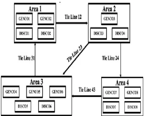
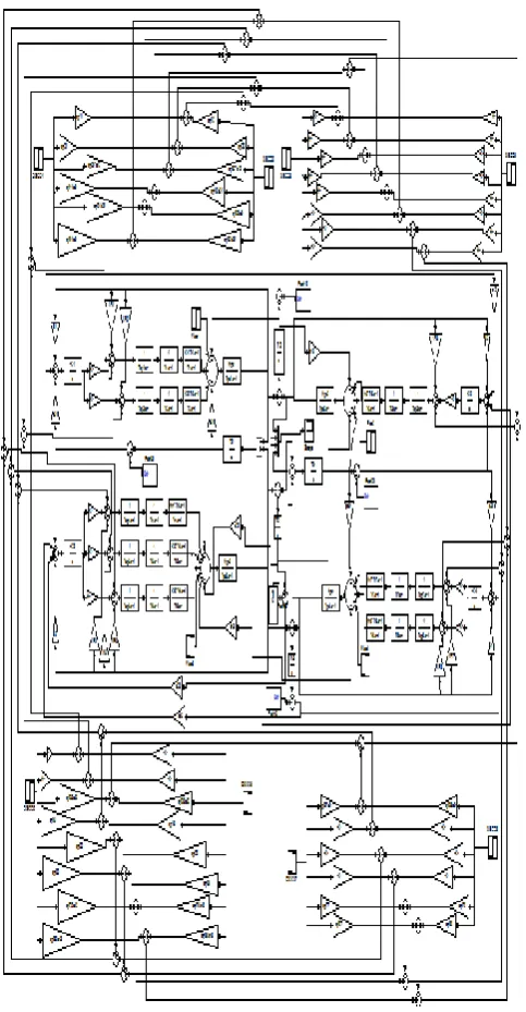
The detailed scheme of the system is given in Fig.1. Consider a four-area system in which let GENCO1, GENCO2, DISCO1 and DISCO2 are in Area 1, GENCO3, DISCO3 and DISCO4 are in Area 2, GENCO4, GENCO5, GENCO6, DISCO5 and DISCO6 are in Area 3 and GENCO7, GENCO8 DISCO7 and DISCO8 are in Area 4 as shown in Fig.1. The full MATLAB-SIMULINK based block diagram for four-area AGC in a deregulated power market is shown in Figure 2.
Figure 1: Schematic diagram of a four area system in restructured power market.
Where cpf represents “contract participation factor”. It
is noted that 1
1
ij i
cpf
. In restructured environment,when the load demand by a DISCO changed, a local load change is observed in the area of the DISCO. This corresponds to the local load power system block. The coefficients, which represent this sharing, are called as
“ACE participation factors” (apf) and 1
1
m j j
apf
where m is the number of GENCOs in the each area. As different from traditional AGC system, any DISCO can demand power from any GENCOs. These demands are determined by cpfs, which are contract participation factor, as load of the DISCO. In the case of two-area power system, scheduled steady state power flow on any tie-line is given as follows:
In the case of four-area power system, scheduled steady state power flow on any tie-line is given as follows :
∆Ptie-linei-j, scheduled = [demand of DISCOs in area j from
GENCOs in area i] - [demand of DISCOs in area i
from GENCOs in area j].
The tie-line power given as follows [10]:
∆Ptie-linei-j,error = ∆Ptie-linei-j,actual - ∆Ptie-linei-j,scheduled (1)
The error signal is used to generate its ACE signal as follow:
ACEi=Bi∆fi + ∆Ptie-linei-j,error (2)
The closed loop two area power system in is characterized in the steady state form as follows:
̇=Acl + Bcl (3)
Where is the state vector and is the vector of
demand of the DISCOs. Acl and Bcl matrixes.
For four area system: ACE participation factors, apf1 =
0.5, apf2 = 0.5, apf3 = 1.0, apf4 = 1/3, apf5 = 1/3, apf6 =
1/3, apf7 = 0.5, apf8 = 0.5. The scheduled load of discos
in different areas, delPdisco1 = 0.3, delPdisco2 = 0.2, delPdisco3 = 0.1, delPdisco4 = 0.4, delPdisco5 = 0.3, delPdisco6 = 0.3, delPdisco7 = 0.3 and delPdisco8 = 0.2. The local loads of Areas 1, 2, 3 and 4 are delPuncot1 = 0.15, delPuncot2 = 0.15, delPuncot3 = 0.2 and delPuncot4 = 0.2, respectively. Ratio of rated powers of
Area 1 and Area 2, a12 = 2.5, ratio of rated powers of
Area 2 and Area 3, a23 = 1/3, ratio of rated powers of
Area 3 and Area 1, a31 = 1.2, ratio of rated powers of
Area 2 and Area 4, a24 = 0.5 and ratio of rated powers of
Area 4 and Area 3, a43 = 1/1.5.
Case 1:
In this scenario GENCOs participate in automatic generation control of their own areas only. It is assumed that large step contracted loads are simultaneously demanded by DISCOs of Areas 1, 2, 3 and 4. A case of Poolco based contracts between DISCOs and available GENCOs is simulated based on the following contract participation factor matrix.
DPM=
0.5 0.5 0 0 0 0 0 0
0.5 0.5 0 0 0 0 0 0
0 0 1 1 0 0 0 0
0 0 0 0 0.3 0.25 0 0
0 0 0 0 0.4 0.5 0 0
0 0 0 0 0.3 0.25 0 0
0 0 0 0 0 0 0.5 0.6
0 0 0 0 0 0 0.5 0.4
Case 2:
In this case, any DISCO has the freedom to have a contract with any GENCO in its own and other areas. Consider that all the DISCOs contract with the available GENCOs for power as per the following matix. All GENCOs participate in the automatic generation control. These GENCOs can supply power to their own area and to other areas also. Also, the ACE participation factor of each GENCO participating in the automatic generation control is defined as follows:
Area 1: apf1 = 0.5, apf2 = 0.5. Area 2: apf3 = 1.0.
Figure 2. The MATLAB simulation model for four-area AGC in a deregulated power market
DPM=
0.2 0.3 0.1 0.1 0.1 0.1 0 0
0.4 0.3 0.1 0.2 0.1 0.1 0 0
0.1 0.1 0.3 0.2 0 0.1 0.1 0.1
0.1 0.1 0.1 0.1 0.2 0.2 0.1 0.1 0.1 0.1 0.1 0.1 0.2 0.2 0.1 0.1 0.1 0.1 0.1 0.1 0.2 0.2 0.2 0.1
0 0 0.1 0.1 0.1 0 0.2 0.3
0 0 0.1 0.1 0.1 0.1 0.3 0.3
Case 3:
In this case, DISCOs may violate a contract by demanding more power than that specified in the contract. This excess power is reflected as a local load of the area (un-contracted demand). Consider Case 2 again. „DPM‟ matrix is the same as in System 2. Total of all DISCOs‟ contracted loads and the un-contracted load of the area are taken up by the GENCOs in the
same area, the scheduled incremental tie-line powers remain the same as in Case 2 in the steady state. Un-contracted load of the area is taken up by the GENCOs of its own area according to ACE participation factors of GENCOs in the steady state.
III.
RESULTS AND DISCUSSION
In this paper, in controller gains at each area in the four-area system in deregulated operation are optimized using PSO. The simulation is done using MATLAB metafile. The cost function J obtains using (1) is given to the PSO technique. Sampling time is chosen as 0.2s. In case 1, the four optimum values of integral gains
found are KI1 = 0.8599, KI2 = 1, KI3 = 0.3832 and KI4 =
0.5663. The dynamic responses of frequency and tie-line power are shown in Fig.3 (a)-(i). In case 2, the four
optimum values of integral gains found are KI1 = 0.6154,
KI2 = 0.2973, KI3 =0.4451 and KI4 = 1. The dynamic
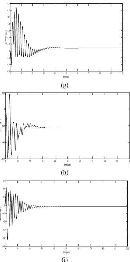
responses of frequency and tie-line power are shown in Fig 4. (a)-(i).In case 3, the four optimum values of
integral gains found are KI1 = 0.2255, KI2 = 0.8132, KI3 =
0.3234 and KI4 = 0.8378. The dynamic responses of
frequency and tie-line power are shown in Fig 5 (a)-(i).
(a)
(b)
0 10 20 30 40 50 60 70 80 90 100 -2
-1.5 -1 -0.5 0 0.5 1 1.5
time (sec)
d
e
lf
1
(H
z)
0 10 20 30 40 50 60 70 80 90 100
-2.5 -2 -1.5 -1 -0.5 0 0.5 1 1.5 2 2.5
time (sec)
d
e
lf
2
(
H
(c) (d) (e) (f) (g) (h) (i)
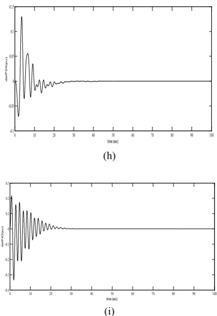
Figure 3. (a) Frequency deviation in area 1. (b) Frequency deviation in area 2. (c) Frequency deviation in area 3. (d) Frequency deviation in area 4. (e) Tie-line power deviation in area 1 and area 2. (f) Tie-line power deviation in area 2 and area 3. (g) Tie-line power deviation in area 3 and area 1. (h) Tie-line power deviation in area 2 and area 4. (i) Tie-line power deviation in area 4 and area 3.
(a)
(b)
0 10 20 30 40 50 60 70 80 90 100 -2.5 -2 -1.5 -1 -0.5 0 0.5 1 1.5 2 time (sec) d e lf 3 (H z)
0 10 20 30 40 50 60 70 80 90 100 -2.5 -2 -1.5 -1 -0.5 0 0.5 1 1.5 time (sec) d e lf 4 (H z)
0 10 20 30 40 50 60 70 80 90 100 -0.15 -0.1 -0.05 0 0.05 0.1 0.15 0.2 time (sec) d e lP 1 2 (p u )
0 10 20 30 40 50 60 70 80 90 100 -0.25 -0.2 -0.15 -0.1 -0.05 0 0.05 0.1 0.15 time (sec) d e lP 2 3 (p u )
0 10 20 30 40 50 60 70 80 90 100
-0.08 -0.06 -0.04 -0.02 0 0.02 0.04 0.06 0.08 time (sec) d e lP 3 1 (p u )
0 10 20 30 40 50 60 70 80 90 100
-0.1 -0.05 0 0.05 0.1 0.15 time (sec) d e lP 2 4 ( p u )
0 10 20 30 40 50 60 70 80 90 100 -0.4 -0.3 -0.2 -0.1 0 0.1 0.2 0.3 time (sec) d e lP 4 3 (p u )
0 10 20 30 40 50 60 70 80 90 100 -2 -1.5 -1 -0.5 0 0.5 1 1.5 time (sec) d e lf 1 (H z)
(c) (d) (e) (f) (g) (h) (i)
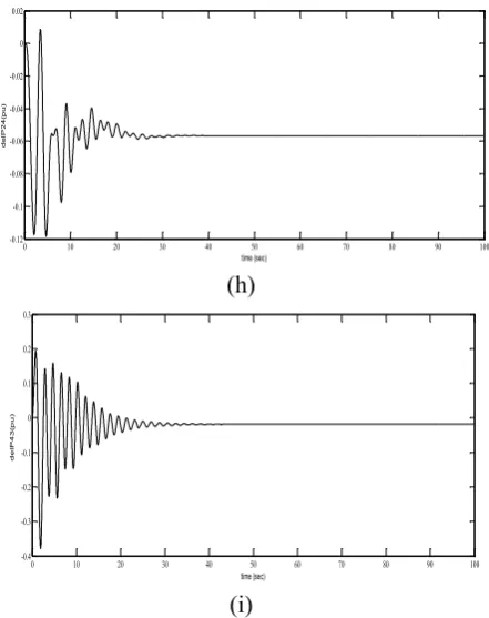
Figure 4. (a) Frequency deviation in area 1. (b) Frequency deviation in area 2. (c) Frequency deviation in area 3. (d) Frequency deviation in area 4. (e) Tie-line power deviation in area 1 and area 2. (f) Tie-line power deviation in area 2 and area 3. (g) Tie-line power deviation in area 3 and area 1. (h) Tie-line power deviation in area 2 and area 4. (i) Tie-line power deviation in area 4 and area 3.
(a)
(b)
0 10 20 30 40 50 60 70 80 90 100 -2.5 -2 -1.5 -1 -0.5 0 0.5 1 1.5 2 time (sec) d e lf 3 (H z)
0 10 20 30 40 50 60 70 80 90 100 -2 -1.5 -1 -0.5 0 0.5 1 1.5 time (sec) d e lf 4 (H z)
0 10 20 30 40 50 60 70 80 90 100 -0.1 -0.05 0 0.05 0.1 0.15 0.2 0.25 time (sec) d e lP 1 2 (p u )
0 10 20 30 40 50 60 70 80 90 100
-0.3 -0.25 -0.2 -0.15 -0.1 -0.05 0 0.05 0.1 time (sec) d e lP 2 3 (p u )
0 10 20 30 40 50 60 70 80 90 100 -0.06 -0.04 -0.02 0 0.02 0.04 0.06 0.08 0.1 time (sec) d e lP 3 1 (p u )
0 10 20 30 40 50 60 70 80 90 100 -0.12 -0.1 -0.08 -0.06 -0.04 -0.02 0 0.02 time (sec) d e lP 2 4 (p u )
0 10 20 30 40 50 60 70 80 90 100 -0.4 -0.3 -0.2 -0.1 0 0.1 0.2 0.3 time (sec) d e lP 4 3 (p u )
0 10 20 30 40 50 60 70 80 90 100
-2.5 -2 -1.5 -1 -0.5 0 0.5 1 1.5 time (sec) d e lf 1 (H z)
(c)
(d)
(e)
(f)
(g)
(h)
(i)
Figure 5. (a) Frequency deviation in area 1. (b) Frequency deviation in area 2. (c) Frequency deviation in area 3. (d) Frequency deviation in area 4. (e) Tie-line power deviation in area 1 and area 2. (f) Tie-line power deviation in area 2 and area 3. (g) Tie-line power deviation in area 3 and area 1. (h) Tie-line power deviation in area 2 and area 4. (i) Tie-line power deviation in area 4 and area 3.
IV.
CONCLUSION
In this paper, AGC of an interconnected power system after deregulation is presented. In deregulated environment, bilateral contracts between DISCOs in one control area and GENCOs in another control area are considered. The elements of DPM are chosen in accordance with bilateral contracts. The AGC is studied for different possible contracts in deregulated
0 10 20 30 40 50 60 70 80 90 100
-3 -2 -1 0 1 2 3
time (sec)
d
e
lf
3
(
H
z)
0 10 20 30 40 50 60 70 80 90 100
-2.5 -2 -1.5 -1 -0.5 0 0.5 1 1.5
time (sec)
d
e
lf
4
(
H
z)
0 10 20 30 40 50 60 70 80 90 100
-0.15 -0.1 -0.05 0 0.05 0.1 0.15 0.2 0.25
time (sec)
d
e
lP
1
2
(
p
u
)
0 10 20 30 40 50 60 70 80 90 100
-0.35 -0.3 -0.25 -0.2 -0.15 -0.1 -0.05 0 0.05 0.1
time (sec)
d
e
lP
2
3
(p
u
)
0 10 20 30 40 50 60 70 80 90 100
-0.06 -0.04 -0.02 0 0.02 0.04 0.06 0.08 0.1 0.12 0.14
time (sec)
d
e
lP
3
1
(
p
u
)
0 10 20 30 40 50 60 70 80 90 100
-0.15 -0.1 -0.05 0 0.05
time (sec)
d
e
lP
2
4
(p
u
)
0 10 20 30 40 50 60 70 80 90 100
-0.5 -0.4 -0.3 -0.2 -0.1 0 0.1 0.2 0.3
time (sec)
d
e
lP
4
3
(
p
u
environment. The scheduled flow on a tie-line between two control areas matches with the contract directions. The dynamic responses obtained for different possible contracts satisfy the AGC requirements.
V.
REFERENCES
[1].Vaibhav Donde, M.A.Pai, Iran. A Hiskens,
"Simulation and optimization in an AGC system after deregulation," IEEE Trans. On Power Syst., vol. 16, no.3, pp. 481-488, August 2001
[2].R. Roy, and S.P. Ghoshal, "Optimized AGC
simulator in deregulated power markets," in Proc. Of National Power System Conf. 2006, IIT, Roorkee, 27-30th December, 2006
[3].Jinn-Tsong Tsai, Liu Tung-Kuan, and Jyh-Horng
Chou, "Hybrid Taguchi-genetic algorithm for global numerical optimization," IEEE Trans. Evol. Comput., vol. 8, no. 4, pp. 365-377, 2004.
[4].S.P. Ghoshal, "Optimization of PID gains by
particle swarm optimization in fuzzy based automatic generation control," Elect. Power Syst. Res., vol. 72, issue 3, pp 203-212, May 2004
[5].Jiejin Cai, Xiaoqian Ma, Lixiang Li, Yixian Yang,