Automatic T-S fuzzy model with application to designing predictive controller

Automatic T-S fuzzy model with application to

designing predictive controller

Zhi-gang Su, Pei-hong Wang, and Yu-fei Zhang

School of energy & environment, Southeast University, Nanjing, Jiangsu 210096, China

[email protected]

Abstract. A novel methodology is proposed to automatically extract T-S fuzzy model with enhanced performance using VABC-FCM algorithm, a novel Variable string length Artificial Bee Colony algorithm (VABC) based Fuzzy C-Mean clustering technique. Such automatic methodology not requires a priori specification of the rule number and has low approximation error and high prediction accuracy with appreciate rule number. Afterward, a new predictive controller is then proposed by using the automatic T-S fuzzy model as the dynamic predictive model and VABC as the rolling optimizer. Some experiments were conducted on the superheated steam temperature in power plant to validate the performance of the proposed predictive controller. It suggests that the proposed controller has powerful performance and outperforms some other popular controllers.

Keywords: T-S fuzzy model, fuzzy c-means; automatic; Artificial Bee Colony; predictive control, superheated steam temperature

1.

Introduction

System modeling and (rolling) optimization are the two main issues to design a predictive controller for an uncertain nonlinear system [27]. In this paper, we aim to propose a novel methodology used to automatically extract model from data and then to design a predictive controller using such novel methodology.

Fuzzy system modeling approach is an effective tool for the approximation of uncertain nonlinear systems on the basis of observed data [13]. Among the different fuzzy modeling techniques, the Takagi-Sugeno (T-S) model [34] has attracted most attention and is popularly applied [12, 14, 28, 30, 32]. The construction of a T-S fuzzy model is generally done in two steps. In the first step, the fuzzy sets in the rule antecedents are determined. This can be done manually, using expert knowledge of the process or by some data-driven techniques. In the second step, the parameters of the consequent functions

1 _{This article is supported by the National natural science foundation of China}

are estimated. As these functions are usually chosen to be linear in their parameters, standard linear least-squares methods can be used. The bottleneck of the construction procedure is the identification of the fuzzy sets in the antecedents. In the traditional T-S fuzzy model, the expert knowledge is used to define linguistically the fuzzy sets, which leads to the drawbacks of subjectivity and suffers lack of generalization. To overcome these issues, reduce expert knowledge intervention and rather build self learning systems, more objective T-S fuzzy models are developed, such as the first family of population stochastic optimization based methods [4, 9, 10, 11, 16, 19, 25, 39] and the second family of clustering based methods [1, 6, 20, 21, 33, 37, 40]. Because of the powerful global search ability of the population stochastic optimization algorithms, this first family of method has high prediction accuracy [15]. Attractive features of the second family of method are the simultaneous identification of the antecedent membership functions along with the consequent local linear models and the implicit regularization [15].

Although the aforementioned approaches improve the efficiency of the T-S fuzzy model, they have various challenges that should not be neglected [35]. The two main challenges among these are how to automatically determine the rule number and to obtain a global optimal model. For the above first family of method, they usually can get a global structure of T-S fuzzy model due to their powerful global search ability. However, they cannot automatically determine the rule number. In some literature [39], the rule number is labeled as a cell in the fixed length of individual so as to automatically determine the rule number. It is crisp in nature. This drawback also exists for the second family of method due to the reason that the cluster number is assumed to be fixed a priori. In addition, the second family of method usually cannot get global optimization solutions, because the traditional fuzzy clustering techniques often get stuck at suboptimal solutions based on the initial configuration. A methodology, used to extract T-S fuzzy model with enhanced performance and without knowing the rule number as a priori, is desirable. In [31], we viewed the fuzzy clustering as an optimization problem where the length of the optimal solution(s) is not known as a priori, and we thus proposed a novel version of Fuzzy C-Means clustering technique, called VABC-FCM algorithm, based on the so-called Variable string length Artificial Bee Colony (VABC) algorithm, another contribution in [31]. By using such novel VABC-FCM algorithm, in this paper, we further propose a novel methodology to automatically extract T-S fuzzy models from data. Use of VABC-FCM allows such methodology not require a priori specification of the rule number and have low approximation error and high prediction accuracy.

derivation methods [14, 22, 27, 32]. Here, we apply the (V)ABC (i.e., VABC or ABC) algorithm as the optimizer, due to the following two reasons [18]: (1) ABC algorithm is recently a popular swarm intelligent algorithm, which outperforms the evolutionary algorithms and other swarm intelligent algorithm in the most of cases; and (2) The number of control parameters involved in ABC is less than that of other population stochastic optimization algorithms. Note that, the (rolling) optimization in predictive control is a constrained optimization problem where the length of optimal solutions is fixed and known as a priori. So, the VABC algorithm and ABC algorithm are equivalent in this case, which will be discussed later in the paper. By using the automatic T-S fuzzy model as the dynamic predictive model and the VABC algorithm as the rolling optimizer, we design a new predictive controller in this paper.

The rest of this paper is organized as follows. Section 2 introduces VABC algorithm and VABC-FCM algorithm. Section 3 presents the automatic T-S fuzzy model. In Section 4, a new fuzzy model predictive controller is designed. The last section concludes this paper.

2.

VABC algorithm and VABC based Fuzzy clustering

2.1. The VABC algorithm

In VABC algorithm, the foraging artificial bees are categorized into three groups: employed bees, onlookers and scouts. The task of each category of bees is also the same as that in the ABC algorithm [17, 18] except for some differences. The main difference is the string or food source representation. In ABC, all the lengths of strings are fixed to be equal, whereas those in VABC are variable. This difference is shown in a d-dimensional space in Fig. 1.

Fig. 1. String representation for (a) ABC and (b) VABC

Firstly, a randomly distributed initial population of n solutions is generated according to mechanism (1).

1 2 ... j ... d

..

.

x1

xn

x2 (a)

..

.

xk

dimension

S

tr

in

g

s

1 2 ... j ... d

..

.

x1

xn

x2 (b)

..

.

xk

dimension

S

tr

in

g

 









    

, min, max, min,

x_{i j} x _j rand , x _j x _j , j , , ,J_i (1)

where Ji is the length of the i th

string and suppose its value is no less than 2. Thus, given a upper bound dmax for Ji (i = 1, 2, ..., n), it can be randomly derived according to:

  







 ,  _max 

i

J round rand d (2)

where each solution xi (i = 1, 2, ..., n) is a d-dimensional vector.

After initialization, the population is subjected to repeated cycles of four major steps: updating feasible solutions, selecting feasible solutions, avoiding suboptimal solutions and solutions mutation.

All employed bees select a new candidate food source position. The choice is based on the neighborhood of the previously selected food source. The position of such new candidate food source is calculated from equation below:

 





    

, , , ,

xnew j xi j rand , xi j xk q (3)

where k  {1, 2, ..., ne} and k ≠ i, and rand[-1, 1] is a uniformly distributed real number in interval [-1, 1]. Subscript j and q denotes respectively the jth and qth

dimension of xi and xk , determined as

  







  







0 1 1 1

0 1 1 1

      

 

    



, ,

, ,

i k i

k

q j round rand J if J J

j q round rand J otherwise

(4)

with round(.) function rounding a number to the nearest integer and the symbol “qj” assigning value of variable j to variable q.

The old food source position in the employed bees’ memory will be replaced by the new candidate food source position, if the new position has a better fitness value. Employed bees will return to their hive and share the fitness value of their new food sources with the onlooker bees.

In the next step, each onlooker bee selects one of the proposed food sources depending on the fitness value obtained from the employed bees. The probability that a food source will be selected can be obtained from following equation:

1







i i l

l

p fit fit (5)

where fiti is the fitness value of the i th

food source xi. Obviously, the higher the

fiti is, the more probability the i th

food source is selected.

In the third step, any food source position that does not improve the fitness value will be abandoned and replaced by a new position that is randomly determined by a scout bee. This helps avoid suboptimal solutions. The new randomly chosen position will be calculated according to Eq. (1).

The final step is a mutation operation on the strings/food sources that are selected for mutation. The mutation operator is defined of three types:

1. If the length of the selected string is longer than that of the string holding the best fitness, one randomly generated cell (i.e., a real-number in a random dimension) is removed from the string.

2. If the length of the selected string is shorter than that of the string holding the best fitness, one randomly generated cell is added to the string. 3. Otherwise, the selected string is hold on.

The mutation probability is selected adaptively for each string as in [29]. Let

fitmax be the maximum fitness,fitbe the average fitness of the population and

fit be the fitness value of the solution to be mutated. The expression for mutation probability, pm, is given below:









1 2

 _{  }

   

max max ,

, m

k fit fit it fit if fit fit p

k otherwise

(6)

where k1 and k2 are constant. Here, both k1 and k2 are kept equal to 0.5. Given a threshold p0 for the mutation, the string is selected when its mutation probability is bigger than p0, i.e., pm > p0. It is evident that p0 cannot be higher than the value of k2, otherwise the mutation operation is useless: once p0 is higher than the value of k2, the length of each string in the population will keep the same as its initial length when the VABC is terminated. In such viewpoint, the VABC algorithm degenerates to ABC algorithm once the lengths of string xi are equally initialized and/or p0 is set to be bigger than k2.

The maximum number of cycles (Cmax) is used to control the number of iterations and is a termination criterion. The process will be repeated until the number of iteration equals the Cmax.

2.2. VABC- FCM: VABC based fuzzy c-means clustering approach

Let Z = {z1, z2, ..., zN} be a collection of vectors in R d

describing N objects. Let

c (2 c N) be the desired cluster number. Each cluster is represented by a prototype or a center vkR

d

. Let V denotes a matrix of size (cd) composed of the coordinates of the cluster centers such that Vkq is the q

th

component of the cluster center vk. FCM looks for a partition matrix U = (uik) of size (Nc) and for the matrix V by minimizing the following objective function:





1 1 1 1

   







, , z v

N c N c

m m

FCM ik ik ik i k

i k i k

subject to the following constraints (8) and (9):





1

1 1 2



  



c

ik k

u i N (8)





1

0 1 2



  



N

ik i

u k c (9)

For a given cluster number c, the algorithm starts from an initial guess for either the partition matrix or the cluster centers and iterates until convergence. Convergence is guaranteed but it may lead to local minimum [2]. To choose optimal cluster number c, clustering validity index is necessary. A sufficient review for fuzzy clustering validity indexes can refer to Refs. [23, 24]. Among them, the most popular two are XB-index [36] and PBM-index [23], defined as:









2 2 1 1

  





, , min v v

c N

ik ik i j i j

k i

XB U V Z u D N (10)









 

c N

i j i j k i ik ik

PBM U V Z E c u D (11)

where E1 is the constant avoiding the PBM to be too smaller. Here, E1 = 100. As can be seen from validity indexes (10) and (11), the cluster number minimizing XB-index leads to the optimal partition of data set Z, and on the contrary, proper fuzzy partitioning can be obtained for a data set by maximizing the PBM-index. Thus, the fuzzy c-means clustering can be viewed as an optimization problem where the best partition is considered to be the one that corresponds to the minimum value of the XB-index or to the maximum value of the PBM-index. Therefore, the framework of the VABC-FCM is the same as that of the VABC algorithm except for some differences, which are interpreted as followings.

The first difference may be the string representation and population of food sources initialization. In VABC-FCM, center based encoding is used where centers are considered to be indivisible. Real numbers are encoded in the strings which represent the coordinates of the centers of the partitions. The length of a particular string xiis nowJi, calculated by

  







 

  _ ,  _max  _

i

J d round rand d (12)

Note that dmax here is the upper bound of the cluster number, not the maximal dimension of data space as interpreted in VABC algorithm. The initial cluster number will therefore range from two to dmax. The centers encoded in a string are randomly selected distinct points from the data set. The selected points are distributed randomly in the string.

The membership value uik in VABC-FCM algorithm is updated by using the same criterion as the FCM algorithm. After obtaining the membership value

criterion as the FCM algorithm. Centers are further updated so as to incorporate a limited amount of local search for speeding up the convergence of VABC-FCM.

The second difference between VABC-FCM algorithm and VABC algorithm is the fitness computation. The fitness in the VABC-FCM algorithm can be calculated as:

 XB-index case: fit1/





The final difference exists in mutation operation on the selected string(s). In VABC algorithm, once the length of the selected string(s) is not equal to that of the string holding the best fitness, one random dimension is removed or increased. However, in VABC-FCM algorithm, the indivisible cell is not one dimension but a cluster center. Thus, one random cluster center is removed or increased when the selected string(s) do not have the best fitness.

With the above interpretations, the VABC-FCM algorithm can be directly derived from VABC algorithm.

3.

Automatic T-S fuzzy model based on VABC-FCM

The typical T-S fuzzy model rule can be described as follow:

Ri : If x isAi, Then 

 

i i i i i i

d d

y f a a x a x a x (13)

where i = 1, 2, ..., NR, NR is the number of fuzzy rules; x = [x1, x2, ..., xd] is the input variable vector for the ith rule, d is the dimension of input variable;

0 1 2

 

  

θ i, ,i i, i

i a a a ad are the consequent parameters; y i

is an output of the ith

fuzzy rule; Ai is a fuzzy variable on product variable space.

Given the input variables x, the fuzzy model output is computed by a weighted mean defuzzification as follows:

1 1

 







i i

i i

y w y w (14)

where the weight strength wi of the i th

rule is calculated as

 





2



 i x exp  x v σ

x

i A i i

w (15)

where μAi is the membership function of Ai, vxi and σi denote the center (or mean) and width (or standard deviation) of the fuzzy set Ai, respectively.

Ri : IF x is in cluster Ci





0 1 1 2 2

    

i i i i i

d d

y a a x a x a x

(16)

where vector ui, the i th

row of membership degree matrix U, is calculated as:

   





1 1 2

   



  /



, , , ,

R N

m m

i u uji ji Dji i Dji j N

u (17)

The following Algorithm 1 depicted the procedure used to automatically extract T-S fuzzy model.

Algorithm 1 VABC-FCM based automatic T-S fuzzy model Identification stage

Input: Input-output Z = [X, y], where X is input matrix and y is output vector. Output: Structure of automatic T-S fuzzy model: {V , U, θ}.

Step 1: Initialization.

Step 2: Apply the VABC-FCM to automatically determine the rule number

NR, the center coordinates V = {vk | k = 1 to NR } of the NR rules, and the membership matrix U = { uik | i = 1 to N }.

Step 3: Determine the local model in each rule by minimizing:









1

  

θ

y θ y θ

min

T

e k k e k

X X

N

where Xe = [1, X] is the matrix extended by a unitary column and the diagonal matrix Φk is defined as:





 k diag u uk, k , ,ukN

Thus, the consequent parameters of the kth local model is given by:





  

θ T T y

k Xe kXe Xe k

Evaluation stage

Input: An arbitrary input z = [x, y] and T-S fuzzy model: {V, U, θ}. Output: Predictionyof x.

Step 1: Calculate the distances between z and center vectors in V;

Step 2: Calculate the membership degrees of sample z belonging to each local model; take the membership degrees as the weights of z belong to the

NR local models

Step 3: Calculate the response yk of x for local model θk, and obtain the predictionyof x.





1







k

MSE y y

N

To show the powerful performance, our proposed method is compared with other advanced T-S fuzzy models as mentioned in the Introduction.

Example 1: Nonlinear static system [33]

The nonlinear static system with two inputs, x1 and x2, and a single output,

y:





2 1 5

1 2 2

1   1 5

   .  

, ,

y x x x x

As in [33], 502 input-output data, consisting of 50 training and testing samples respectively, are used. With the 50 input-output training samples, the automatic T-S fuzzy model can be constructed. The experiments are run for 50 times. The automatic T-S fuzzy model for random one of the 50 running times is presented as follows.

R1: IF x is in C1 ((1.2721, 1.4796), u1)

Then 1

1 2

2.6648 0.7508 0.7408

y x x

R2: IF x is in C2 ((2.6415, 2.0677), u2) Theny24.1955-0.2718 -0.6389x1 x2

R3: IF x is in C3 ((4.302, 4.3758), u3)

Then 3

1 2

0.9269 0.0274 0.0542

y x x

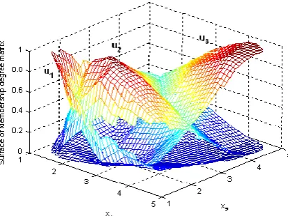
where u1, u2 and u3 among the rules R1, R2 and R3 are indicated in Fig. 2.

Fig. 2. Membership matrix for the nonlinear static system by using VABC-FCM algorithm

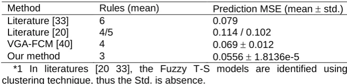
Fig. 3 shows the prediction of the T-S fuzzy model and the prediction errors for the 50 testing samples. In this case, the training MSE is 0.024911, and the prediction/testing MSE is 0.055616.

the other three advanced methods [20, 33, 40] are also run here. The results are presented in Table 1. It suggests from Table 1 that our method has high prediction accuracy with appreciated rules.

0 5 10 15 20 25 30 35 40 45 50

1 2 3 4 5 6

Sample index

O

u

tp

u

t

o

f

m

o

d

e

l

Target Model

0 5 10 15 20 25 30 35 40 45 50

-1 -0.5 0 0.5

Sample index

e

(t

)

Fig. 3. Predictions of the 50 testing samples using automatic T-S fuzzy model

Table 1. Comparison results for nonlinear static system*1

Method Rules (mean) Prediction MSE (mean  std.)

Literature [33] 6 0.079

Literature [20] 4/5 0.114 / 0.102

VGA-FCM [40] 4 0.069  0.012

Our method 3 0.0556  1.8136e-5

*1 In literatures [20 33], the Fuzzy T-S models are identified using clustering technique, thus the Std. is absence.

Example 2: Box-Jenkins (BJ) gas furnace [3]

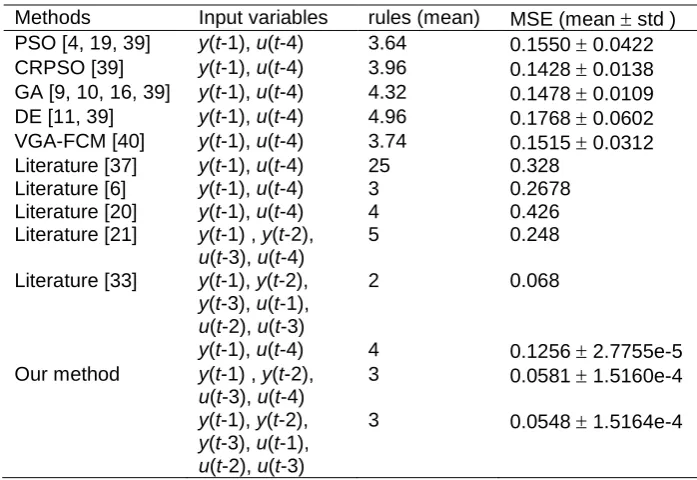
This example uses BJ gas furnace data to show the approximation ability of the proposed model. The model holding lower approximation error with fewer rules is the best one. The BJ dataset, recorded from a combustion process of a methane-air mixture, has been used widely to validate the performance of the new proposed modeling methods. There are originally 296 data points, t = 1 to 296. y(t) is the output CO2 concentration and u(t) is the input gas flowing rate. It has been found in the most literatures that three popular sets of input variables for predicting y(t): (1) y(t-1) and u(t-4), (2) y(t-1), y(t-2), u(t-3) and

u(t-4), and (3) y(t-1), y(t-2), y(t-3), u(t-1), u(t-2) and u(t-3). All these three kinds of input variables are considered in our study.

in Table 2, as well as the Std. values of the MSE. In Table 2, we also present the results obtained by using other advanced methods. It shows that our proposed method outperforms other methods.

Table 2. Comparison results for BJ gas furnace data set

Methods Input variables rules (mean) MSE (mean  std )

PSO [4, 19, 39] y(t-1), u(t-4) 3.64 0.1550  0.0422

CRPSO [39] y(t-1), u(t-4) 3.96 0.1428  0.0138

GA [9, 10, 16, 39] y(t-1), u(t-4) 4.32 0.1478  0.0109

DE [11, 39] y(t-1), u(t-4) 4.96 0.1768  0.0602

VGA-FCM [40] y(t-1), u(t-4) 3.74 0.1515  0.0312

Literature [37] y(t-1), u(t-4) 25 0.328

Literature [6] y(t-1), u(t-4) 3 0.2678

Literature [20] y(t-1), u(t-4) 4 0.426

Literature [21] y(t-1) , y(t-2),

u(t-3), u(t-4)

5 0.248

Literature [33] y(t-1), y(t-2),

y(t-3), u(t-1),

u(t-2), u(t-3)

2 0.068

y(t-1), u(t-4) 4 0.1256  2.7755e-5

Our method y(t-1) , y(t-2),

u(t-3), u(t-4)

3 0.0581  1.5160e-4

y(t-1), y(t-2),

y(t-3), u(t-1),

u(t-2), u(t-3)

3 0.0548  1.5164e-4

4.

Application to design fuzzy predictive controller

Section 4.1 shows the procedures used to design predictive controller. Consequently, some experiments are conducted to validate the performance of the designed predictive controller in section 4.2.

4.1. Automatic T-S model and (V)ABC based predictive controller

There are various families of strategies used to design predictive controller since the basic concept of predictive control is proposed [26]. Although there exist differences in assumptions and designing ideas, the key idea of these strategies are similar. More precisely, for a given Single Input (control input or controller output u) Single Output (process output or plant output y) system (SISO) illustrated in Fig. 4, such key idea can be interpreted as follows:

collected, the dynamic predictive model and the assumed control input trajectory {v(t), v(t+1), …, v(t+Nu-1)} for a appreciated time horizon [t, t+Nu-1] (i.e., Nu is generally smaller than the prediction horizon Np);

Select optimal control sequence {v*(t), v*(t+1), …, v*(t+Nu-1)} in the assumed input trajectory v to make the plant outputsyˆ approximate the reference trajectory yr as possible. Such approximation can be realized by minimizing a objective function, generally defined as:

















1  0



  







min Np Nu

r

k k

J y t k y t k v t k

where, Δv(t+k) = v(t+k) - v(t+k-1), yr is reference trajectory and λ is constant weight vector.

Apply the first element of the optimal control sequence v* as the actual control input signal to the plant, i.e., u(t) = v*(t);

Repeat the above operations, once the later sampling time comes.

further past

Set point

yr(t+k)

y(t-1)

u(t-1)

v(t+k)

 

ˆ y tk

t t+1 t+Nu t+Np Control horizon

Prediction horizon

Fig. 4. Key idea of predictive control strategy by using SISO system

In practice, the plant (i.e., object) to be controlled is much more complex and Multiple Inputs Multiple Outputs (MIMO) system is usually faced. In this case, the MIMO can be viewed as the composition of some subsystems with multiple inputs and single output (MISO). By comparing with SISO, note that the MISO only has some more inputs. To avoid confusion with scalar variables such as u, v, y, yr andyˆin the SISO, the corresponding vector variables are denoted by u, v, y, yr andyˆin MIMO system. In what follows, the predictive controller is designed for MIMO system in general.

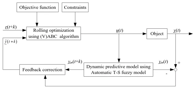
According to the above key idea, we can see that there are three significant characteristics for the model predictive control algorithm: dynamic predictive model, rolling optimization and feedback correction. In our study, the above key idea is also applied. The predictive controller is designed according to the following four steps.

For a given MIMO system, the predictive controller is designed as shown in Fig. 5. It can be seen that the structure maintains the three significant characteristics, holding by the traditional predictive controller. The two main differences are the applications of automatic T-S fuzzy model and (V)ABC algorithm respectively as the dynamic prediction model and rolling optimizer.

Objective function

Rolling optimization using (V)ABC algorithm

Constraints

Feedback correction Dynamic predictive model using Automatic T-S fuzzy model

Object

r(t+k)

u(t)

ym(t+k) ym(t)

y(t)

+

- 

ˆ y tk

Fig. 5. Structure diagram of the designed predictive controller

(2) Dynamic predictive model by using automatic T-S fuzzy model

For MIMO system with ni inputs and no outputs, the dynamic predictive model holds the following form in general:

 





 









 









m y u

y t f y t y t y t n u t u t u t n (18)

where f(.) is the (nonlinear) function describing the plant system, nu and ny are the orders of inputs and outputs respectively, u(t-k) and y(t-k) are respectively the control input vector and plant/object output vector, defined respectively as

































1 1

 

 _    _

 

 _    _

, , , ,

, , , ,

u

o

T

j n

T

i n

u t k u t k u t k u t k

y t k y t k y t k y t k

Such general form (18) can be decomposed into number of no subsystems with ni inputs and single output. Thus, we have

 





























































1 1 1

2 1 2

1 1

1 1

1 1

 _{   } 

 

 _{   } 

 



 

 

 _{   } 

 

, , , , ,

, , , , ,

, , , , ,

o o o

y u

y u

m

n n n y u

f y t y t n u t u t n

f y t y t n u t u t n

y t

f y t y t n u t u t n

(19)

where fi(.) is the dynamic predictive model for the ith MISO subsystem.

we apply the automatic T-S fuzzy model as the dynamic predictive model fi(.) due to its powerful approximation ability and prediction ability, as already discussed in Section 3. Once the input variables of the automatic T-S fuzzy model are determined, the automatic T-S model can be identified to predict the outputs of the object in the further by using the information of these input variables collected at the past and current states. The way how to establish and identify the automatic T-S fuzzy model can refer to Section 3.

(3) Feedback correction strategy

As we known, the performance of automatic T-S fuzzy model may be degenerated along with the running times, although the automatic T-S fuzzy model holds powerful approximation and prediction abilities. This is because the automatic T-S fuzzy model may be established under limited information, i.e., the information is collected at the past and current states. Along with the running times, some new useful information maybe occurs. As well, the characteristics of the object maybe change along with the running times. For instance, characteristics of the object will degenerate when the service life of object is closed. In addition, it is unfeasible to frequently identify the dynamic predictive model in practice. Therefore, feedback correction is necessary.

In this study, we feed back the prediction error and apply it to correct the output of the dynamic predictive model. More precisely, we have





 





 







  









  







1 1

1

1 1

   

      

 

  

 _{    } 

 

ˆ

ˆ , ,ˆ , , , ,

, , ,

, , , , ,

m

y

p u

y t k e t y t k

y t k y t y t y t k n

e t f k N

v t k v t u t u t k n

(20)

where u(t+k-nu), …, u(t-1) are the actual input trajectory at the past cases,

v(t), …, v(t+k-1) are the assumed control input trajectory at the current and further cases, and e(t) is the feedback prediction error defined as:

 

 

 

 





















(4) Rolling optimization by using (V)ABC algorithm

The rolling optimization aims to find the optimal control sequence {v*(t+k) | k

= 0, 1, …, Nu-1} under the following two constraints:

Input constraint: umin v t





To apply the (V)ABC as the optimizer, we should encode the assumed control inputs v as population of food sources in advance. The lth food source can be encoded in the following form:

 

















 

_       _

x l T, l T, , l T, l T, , l T

l v t v t v t k v t k v t Nu

(24)

where







 







T

l l l l

n u

v t k v t k v t k v t k k N

To satisfy the two constraints in Eqs. (22) and (23) simultaneously, it is unfeasible to produce the food sources by applying operation in Eq. (1). Here, the initial population of control inputs at time t is determined according to

 









 





j j j j j i

v t u u u t rand u j (25) n

and the control inputs at other times are defined according to













 





l l

j j j j j

v t k u u v t k rand u (26)

where, k = 1 to Nu, uj, min, uj, max and Δuj, max are the jth element of the umin, umax and Δumax, respectively.

Note that, the new produced candidate food source xnew by applying operation (3) might not satisfy the input move constraint. This situation can be avoided by using the following correction mechanism for each input variable j.

If 









new new

j j j

v t k v t k u , we have













new new

j j j

v t k v t k u ;

If









new new

j j j

v t k v t k u

       , we have













new new

j j j

v t k v t k u .

Once the assumed control inputs are encoded as population of food sources, the rest task is to design an objective function for the rolling optimization. For convenience, we apply the quadratic function, defined as:

1









MIMO i i

i

J J (27)

where γi are constant weights, and Ji is the quadratic objective function of the

ith MISO system and is defined as













0

1

2 2

0

 

 







N N

i r i i i i

k N k

J y t k y t k v t k

(28)

where N0 is time delay, reference trajectory yr, i(t+k) = αi, ky(t) + (1 - αi, k)ysp, i,

The following Algorithm 2 shows the steps to realize the proposed predictive controller.

Algorithm 2: Automatic T-S model & (V)ABC based predictive controller 1. Initialization

Predetermine the parameters such as prediction horizon Np, control horizon

Nu, weight coefficients γi and λi, the limits of control input umin, umax and Δumax, and the control parameters n, dmax, P0 and Cmax in VABC.

2. At time t, read the information such as the plant outputs y(t-1), …, y(t

-ny) and actual control inputs u(t-1), …, u(t-nu).

3. Generate the population of food sources for the current time t.

4. By taking Eq. (27) as the objective function, the optimal assumed control input trajectory {v*(t+k) | k = 0, 1, …, Nu-1} are obtained by using the (V)ABC algorithm.

5. Apply the first element of the optimal control sequence v* as the actual control input to the plant, i.e., u(t) = v*(t).

6. Go to the second step and repeat the operations interpreted in steps 2 ~ 5, when the new state comes, i.e., t = t + 1.

To implement the Algorithm 2, some parameters should be predetermined such as Np, Nu, γi, λi, umin, umax, Δumax, n, dmax, P0 and Cmax. Among them, the latter four parameters can be initialized as that done in [31]. The weight coefficients λi are used to reduce the influence of large changing in control input. If the control system is stable and the changing in control input is not large, the coefficients λi can take a relatively smaller value. On the contrary, large value can be taken by λi. In our method, the coefficients λi can take a small value because the control input has been restricted in a certain interval in advance, as shown in Eqs. (22) and (23). Here, coefficients λi = 0.5 for i= 1 to no. The weight coefficients γi are used to indicate the importance of each sub objective function Ji. Here, γi = 1 for i= 1 to no, because we consider all the objective functions Ji play the same contribution.

4.2. Superheated steam temperature control system

Continuous process in power plant and power station are complex systems characterized by nonlinearity, uncertainty and load disturbance. The superheater is an important part of the steam generation process in the boiler-turbine system, where steam is superheated before entering the boiler-turbine that drives the generator.

Superheater is made of material that have characteristic of high temperature resistant during normal operation, and the average temperature of superheater is close to highest permitted temperature of material. It will result in malfunction and damage when superheater is overheated. On the other hand, when superheated steam temperature is too low, it will reduce the thermal efficiency of power plant and influence the safe operation of turbine. Therefore, superheated steam temperature is one of the most important factor determining the safety and economic of thermal power plant.

Wa1(s) Wa2(s) Wo1(s) Wo2(s)

WH2(s)

WH1(s)

disturbance

Main controller

Secondary

controller Leading section Inertial section

r + u

-+

-+ _y

Fig. 6. Structure of superheated steam temperature control system

Sources of disturbances, affecting the superheated steam temperature, are various, such as, the steam flow, combustion conditions of boiler, enthalpy of steam entering the superheater, the change of temperature and flow speed of fume that flows through the superheater, etc. It is difficult to reach small dynamic deviation. Moreover, the temperature adjustment of export steam is required to prevent the superheater been overheated. At present the Spray Water control strategy is adopted as steam temperature adjustment approach for most thermal power plants. In such case, the input, denoted as u(t), is the amount of Spray Water (kg/s), and the output, denoted as y(t), is the superheated steam temperature (°C). Thus, the structure of superheated steam temperature control system can be interpreted in Fig. 6.

Some parameters of the superheated steam system in Fig. 6 are presented as follows [5]:

 





 





 

 

 

1 2 2 3

1 2 2

8 1 125

1 15 1 25

0 1 0 1 25

.

/ , /

. / , . / ,

o o

H H a

W s C mA W s C mA

s s

W s mA C W s mA C W s

   

 

    

 

 

 

 

 

 

 

 

1 1 2

5 4 3 2

1

22 5

3516000 890625 401250 41850 1605 21

 



    

.

a o o H

a o H

W s W s W s W s G s

W s W s W s

s s s s s

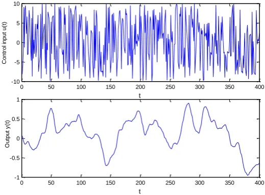
To simulate for the superheated steam temperature system (see in Fig. 6), suppose the input u(t)[-10, 10] , i.e., umin = -10, umax =10, is generated from a pseudo random signal generator The sampling period is set as 5 second (s) and we continuously record a set of samples for 2000 seconds. In other word, four hundreds of points of signals u(t) are collected. Corresponding to the input u(t), the output y(t) can be obtained by using some ways. An intuitionistic way is to deduce y(t) in the SIMULINK environment in MATLAB software according to the calculus G(s). Fig. 7 shows the input t u(t) and output y(t) generated by using this way.

0 50 100 150 200 250 300 350 400

-10 -5 0 5 10

t

C

o

n

tr

o

l i

n

p

u

t

u

(t

)

0 50 100 150 200 250 300 350 400

-1 -0.5 0 0.5 1

t

O

u

tp

u

t

y

(t

)

Fig. 7 The output and input of training samples

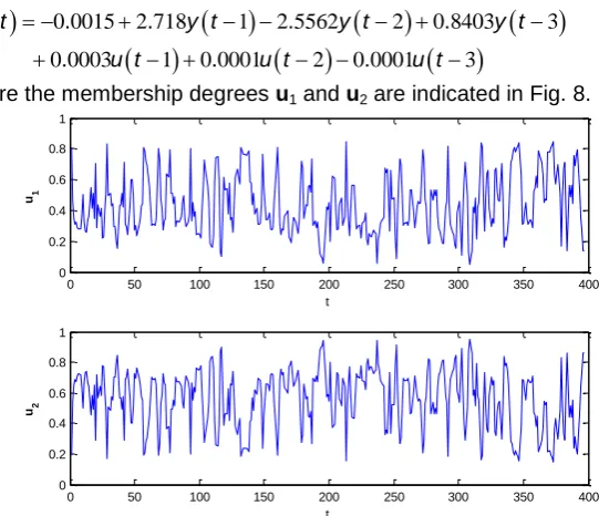
By selecting x = [y(t-1), y(t-2), y(t-3), u(t-1), u(t-2) , u(t-3)] as the input variables (i.e., ny = nu = 3) and y(t) as the output, thus the amount of 400 training samples can be constructed. By using these samples, the automatic T-S fuzzy model can be constructed for the superheated steam temperature, as follows.

R1: If x is in C1 ((-0.9556, -0.9556, -0.9556, -2.7559, -3.0635, -3.6739), u1) Then

 

























0 0015 2 718 1 2 5562 2 0 8403 3

0 0003 1 0 0001 2 0 0001 3

       

     

. . . .

. . .

m

y t y t y t y t

u t u t u t

 

























0 0015 2 718 1 2 5562 2 0 8403 3

0 0003 1 0 0001 2 0 0001 3

       

     

. . . .

. . .

m

y t y t y t y t

u t u t u t

where the membership degrees u1 and u2 are indicated in Fig. 8.

0 50 100 150 200 250 300 350 400

0 0.2 0.4 0.6 0.8 1

t

u1

0 50 100 150 200 250 300 350 400

0 0.2 0.4 0.6 0.8 1

t u2

Fig. 8 Membership degrees distribution of 2 clusters for the superheated steam temperature

With the above established dynamic predictive model, we still should predetermine the prediction horizon and control horizon. According to the discussions about these two parameters in Section 4.1, here we assume Nu = 1 and Np = 10 by considering the fact that the superheated steam temperature system is not too complex and does not have system time delay, i.e., N0 = 0.

To validate the performance of our method, the generalized predictive controller (GPC) [7, 8] and the traditional PI controller are also studied. The prediction horizon Np and control horizon Nu taken by GPC are the same as that in our method. The main controller for the traditional PI is designed as

 

1 1

1 0 5 74

 

 _  _

 

. a

W s

s .

Four typical study cases are conducted to show whether our method is robust or not when the disturbance, prediction horizon, inertial coefficient and gain increase respectively.

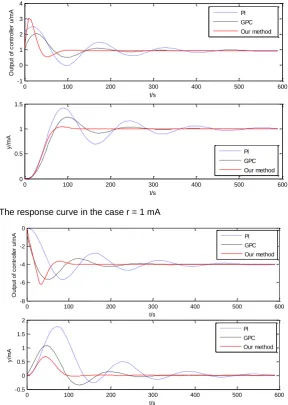
Case 1: Study on the influence of step disturbance

In this case, we analyze the laws how the step changes of reference value (r) and disturbance (d) influence on the performance of our method. Fig. 9 shows the results when r = +1 mA, and Fig. 10 shows the results when d = +4

0 100 200 300 400 500 600 -1

0 1 2 3 4

t/s

O

u

tp

u

t

o

f

c

o

n

tr

o

lle

r

u

/m

A

0 100 200 300 400 500 600

0 0.5 1 1.5

t/s

y

/m

A

PI GPC Our method

PI GPC Our method

Fig. 9 The response curve in the case r = 1 mA

0 100 200 300 400 500 600

-8 -6 -4 -2 0

t/s

O

u

tp

u

t

o

f

c

o

n

tr

o

lle

r

u

/m

A

0 100 200 300 400 500 600

-0.5 0 0.5 1 1.5 2

t/s

y

/m

A

PI GPC Our method

PI GPC Our method

Fig. 10 The simulations under the condition disturbance = +4 mA

Case 2: Study on the influence of prediction horizon

0 200 400 600 -8

-7 -6 -5 -4 -3 -2 -1 0

t/s

O

o

u

tp

u

t

o

f

c

o

n

tr

o

lle

r

u

/m

A

0 200 400 600

-0.8 -0.6 -0.4 -0.2 0 0.2 0.4 0.6 0.8

t/s

y

/m

A

Np=16

Np=10

Np=10 Np=16

Np=6 Np=6

Fig. 11 Influence of Np on results under the condition disturbance = 4 mA and

Case 3: Study on the influence of inertial coefficient

The dynamic characteristics of superheated steam temperature always vary with the changing working conditions. By considering this fact, we want to see whether our method is valid or not when the parameters (i.e., the inertial coefficient in Wo2) of the superheated steam temperature system change in a large range. In other words, we analyze whether our method is sensitive to the inertia of the object or not. To study on the influence of inertial coefficient, we suppose Wo1(s) is unchanged and the inertial coefficient in

Wo2(s) increases from 25 to 35, i.e., the Wo2(s) is redefined as follows (Note that the established automatic T-S fuzzy model is not repeatedly identified according to training samples derived from the following redefined transfer function):

 





2 3

1 125 1 35

  

 .

/ o

W s C mA

s

0 200 400 600 -7 -6 -5 -4 -3 -2 -1 0 t/s O u tp u t o f c o n tr o lle r u /m A

0 200 400 600 -1 -0.5 0 0.5 1 1.5 2 t/s y /m A PI GPC Our method PI GPC Our method

Fig. 12 Results in the case when the inertia of the object increases

Case 4: Study on the influence of gain

In this case, we want to see whether the proposed method is sensitive to the change of gain or not. We suppose Wo1(s) is unchanged and gain in

Wo2(s) increases from 1.125 to 1.875, i.e., the Wo2(s) is redefined as:

 





W s C mA

s

The simulation results are shown in Fig. 13. It can be seen from Fig. 13 that our method is robust in the changes of gain and its performance outperforms the traditional PI and GPC.

0 200 400 600

-8 -7 -6 -5 -4 -3 -2 -1 0 t/s O u tp u t o f o n c tr o lle r u /m A

0 200 400 600

-1 -0.5 0 0.5 1 1.5 2 t/s y /m A PI GPC Our method PI GPC Our method

Fig. 13 Results in the case when proportional gain increases from 1.125 to 1.875

In the study cases 3 and 4, the inertial coefficient and gain can also decrease and we have the similar results as above two study cases.

5.

Conclusions

In this study, a novel methodology for automatically extracting T-S fuzzy model with enhanced performance is proposed by using a novel swarm intelligent fuzzy clustering technique, i.e., the Variable string length Artificial Bee Colony (ABC) algorithm based Fuzzy C-Mean clustering (VABC-FCM). Use of the VABC-FCM algorithm makes the proposed methodology can automatically evolve the rule number from data without knowing the rule number as a priori. Moreover, the output fuzzy partition matrix of VABC-FCM is sufficiently applied in the identification process of T-S fuzzy model, which brings the convenience for model construction and reduces the approximation error. Some numerical examples are used to validate the proposed T-S fuzzy model. The results suggest that it has high prediction accuracy with appreciated rule number.

Consequently, a new fuzzy model predictive controller is designed by using the proposed T-S fuzzy model as its dynamic predictive model and by using (V)ABC algorithm as its rolling optimizer. Taking the superheated steam temperature in power plant as the example, some experiments were conducted to validate the performance of the proposed fuzzy model predictive controller. The experimental results show that the proposed fuzzy model predictive controller has powerful performance. In addition, we compare our method with the popular generalized predictive controller and PI. It shows that our method outperforms the generalized predictive controller and traditional PI controller.

References

1. Babuska, R.. Fuzzy modeling for control. Kluwer Academic Publisher, Boston. (1998)

2. Bezdek, J.C.. Pattern recognition with fuzzy objective function algorithms. Plenum, New York. (1981)

3. Box, G.E.P., Jenkins, G.M.. Time series analysis, forecasting and control. Sanfrancisco, CA: Holden Day. (1970)

4. Chen, C.C.. A PSO-based method for extracting fuzzy rules directly from numerical data. Cybern. Syst. Vol. 37, No. 7, 707-723. (2006)

5. Chen, L.J.. Principle of automatic control in thermal process (in chiness). Water Resources and Electric Power Press, Beijing. (1982)

6. Chen, J.Q., Xi, Y.G., et al.. A clustering algorithm for fuzzy model identification. Fuzzy sets and systems, Vol. 38, 319-329. (1998)

7. Clarke, D.W., Mohtadi, C., Tuffts, P.S.. Generalized predictive control: Part 1, the basic algorithm. Automatica, Vol. 23, 137-148. (1987)

8. Clarke, D.W., Mohtadi, C., Tuffts, P.S.. Generalized predictive control: Part 2, extensions and interpretations. Automatica, Vol. 23, 149-160. (1987)

10. Cordon, O., Herrera, F., Gomide, F., Hoffmann, F., Magdalena, L.. Ten years of genetic fuzzy systems: current framework and new trends. In: proceedings of IFSA and NAFIPS, Vol. 3, 1241-1246. (2001)

11. Eftekhari, M., Katebi, S.D., Karimi, M., Jahanmiri, A.H.. Eliciting transparent fuzzy model using differential evolution. Applied soft computing, Vol. 8, 466-476. (2008) 12. Fisher, M., Nelles, O., Isermann, R.. Adaptive predictive control of a heat

exchanger based on a fuzzy model. Control Eng. Practice, Vol. 6, 259-269. (1998) 13. Hellendoorn, H., Driankov, D.. Fuzzy model identification: selected approaches.

Springer, Berlin, Germany. (1997).

14. Jiang, H., Kwong, C.K., Chen, Z., Ysim, Y.C.. Chaos particle swarm optimization and T-S fuzzy modelling approaches to constrainted predictive control. Expert systems with applications, Vol. 39, 194-201. (2012)

15. Johamsen, T.A., Babuska, R.. On multi-objective identification of Takagi-Sugeno fuzzy model parameters. In preprint 15th IFAC congress, Barcelona, Spain. (2002).

16. Kang, S.J., Woo, C.H., Hwang, H.S., Woo, K.B.. Evolutionary design of fuzzy rule base for nonlinear system modeling and control. IEEE Transaction on Fuzzy Systems, Vol. 8, No. 1, 37-45. (2000)

17. Karaboga, D.. An idea based on honey bee swarm for numerical optimization. Technical report-TR06, Erciyes University, Engineering faculty, Computer Engineering Department. (2005)

18. Karaboga, D., Basturk, B.. On the performance of artificial bee colony (ABC) algorithm. Applied soft computing, Vol. 8, No. 1, 687-697. (2008)

19. Khosla, A., Kumar, S., Aggarwal, K.K.. A framework for identification of fuzzy models through particle swarm optimization. In: IEEE Indicon Conference, Chennai, India, 388-391. (2005)

20. Li, N., Li S.Y., Xi, Y.G.. Multi-model modeling method based on satisfactory clustering. Control theory & application, Vol. 20, No. 5, 783–787. (2003)

21. Lv, J.H., Chen, J.Q., Liu, Z.Y., et al., A study on fuzzy rules based and nonlinear models for thermal processes. Proceedings of the Chinese society for electrical engineering, Vol. 22, No. 11, 132-137. (2002)

22. Martinez, M., Senent, J.S., Blasco, X.. Generalized predictive control using genetic algorithms. Engineering applications of artificial intelligence, Vol. 11, 355-367. (1998)

23. Maulik, U., Bandyopadhyay, S.. Performance evaluation of some clustering algorithms and validity indices. IEEE Transactions on pattern Anal. Machine intelligent, Vol. 24, No. 12, 1650-1654. (2002)

24. Pakhira, M.K., Bandyopadhyay, S., Maulik, U.. Validity index for crisp and fuzzy clusters. Pattern recognition, Vol. 37, No. 3, 487-501. (2004)

25. Pedrycz, W., Reformat, M.. Evolutionary fuzzy modeling. IEEE Transaction on Fuzzy Systems, Vol. 11, No. 5, 652-665. (2003)

26. Richalet, J., Rault, A., Testud, J.L., Papon, J.. Model predictive heuristic control Application to industrical processes. Automatica, Vol. 14, 413-428. (1978)

27. Sarimveis, H., Bafas, G.. Fuzzy model predictive control of non-linear processes using genetic algorithms. Fuzzy sets and systems, Vol. 139, 59-80. (2003)

28. Sousa, J.M., Babuska, R., Verbuggen, H.B.. Fuzzy predictive control applied to an air-conditioning system. Control Eng. Practice, Vol. 5, 1395-1406. (1997)

30. Su, B., Chen, Z., Yuan, Z.. Constrained predictive control based on T-S fuzzy model for nonlinear system. Journal of systems engineering and electronics, Vol. 18, 95-100. (2007)

31. Su, Z.G., Wang, P.H., Shen, J., Li, Y.G., Zhang, Y.F., Hu, E.J.. Automatic fuzzy partitioning approach using Variable string length Artificial Bee Colony (VABC) algorithm. Applied soft computing, Vol. 12, No. 11, 3421-3441. (2012)

32. Sugeno, M., Kang, G.T. Fuzzy modeling and control of multilayer incinerator. Fuzzy sets and systems, Vol. 1, No. 8, 329-346. (1986)

33. Sugeno, M., Yasukawa, T.. A fuzzy logic based approach to qualitative modeling. IEEE Transaction on Fuzzy Systems, Vol. 1, No. 1, 7–31. (1993)

34. Takagi, T., Sugeno, M.. Fuzzy identification of systems and its application to modeling and control. IEEE Transactions on Systems, Man and Cybernetics, Vol. 15, No. 1, 116–132. (1985)

35. Turksen, I.B., Celikyilmaz, A.. Comparison of fuzzy functions with fuzzy rule base approaches. Int. J. Fuzzy Syst, Vol. 8, No. 3, 137-149. (2006)

36. Xie, X.L., Beni, G.. A validity measure for fuzzy clustering. IEEE Transaction on pattern Anal. Machine intelligent, Vol. 13, No. 8, 841-847. (1991)

37. Xu C.W., Yong, Z.. Fuzzy model identification and self-learning for dynamic systems. IEEE Transactions on Systems, Man and Cybernetics, Vol. 17, No. 4, 683–689. (1987)

38. Zhang, Y.F., Su, Z.G., Wang, P.H.. A convenient version of T-S fuzzy model with enhanced performance. In: proceedings of the 8th international conference on Fuzzy Systems and Knowldege Discovery, 1074-1079. (2011)

39. Zhao, L., Qian, F., Yang, Y.P., et al.. Automatically extracting T-S fuzzy models using cooperative random learning particle swarm optimization. Applied soft computing, Vol. 10, 938-944. (2010)

40. Zhu, H.X.. A study on fuzzy modeling and control based on immune optimization algorithms for thermal processes. MS thesis, Southeast University at Nanjing, (2005)

Zhi-gang Su received his M.S. and Ph.D. degrees from Southeast University, Nanjing, China in 2006 and 2010, respectively. He worked with Southeast University from 2010. His research interests are focused on intelligent modeling, machine learning, soft computing and optimization algorithm, as well as their applications.

Pei-hong Wang is a full professor with School of Energy & Environment, Southeast University. His research interests are focused on intelligent modeling, diagnosis and optimization algorithm, as well as the applications of these methods in power plant.

Yu-fei Zhang is an associate professor with School of Energy & Environment, Southeast University. Her research interests are focused on intelligent modeling and control, as well as their applications.