RILL EROSION WITH STRUCTURE FROM MOTION
by Nicholas Ellett
A thesis
submitted in partial fulfillment of the requirements for the degree of
Master of Science in Geoscience Boise State University
DEFENSE COMMITTEE AND FINAL READING APPROVALS
of the thesis submitted by
Nicholas Ellett
Thesis Title: Partitioned by Process: Measuring Post-Fire Debris Flow and Rill Erosion with Structure from Motion
Date of Final Oral Examination: 08 March 2019
The following individuals read and discussed the thesis submitted by student Nicholas Ellett, and they evaluated his presentation and response to questions during the final oral examination. They found that the student passed the final oral examination.
Jennifer Pierce, Ph.D. Chair, Supervisory Committee Nancy Glenn, Ph.D. Member, Supervisory Committee Jaime R. Goode, Ph.D. Member, Supervisory Committee
iv
ACKNOWLEDGEMENTS
v
In mountainous regions burned by wildfires, profound changes in soil characteristics and combustion of vegetation increase hillslope and channel erosion during storm events. Reduced infiltration and abundant loose sediment produce large post-fire erosional events which endanger human lives and infrastructure and contribute significantly to long-term erosion rates. While the influence of fire in increasing erosion has long been recognized, quantifying volumes and sources of eroded material from burned landscapes is difficult. Pre-erosion high-resolution topographic data (e.g. lidar) are often not available in burned areas and determining specific contributions from post-fire hillslope and channel erosion is challenging. Multiple erosional processes mobilize sediment from hillslopes, but the connectivity of hillslopes to channels controls the basin-wide erosional response.
vi
debris flow scour’s geomorphic signature and used a DEM of difference (DoD) to map and quantify channel erosion, finding 3467 ± 422 m3 was eroded by debris flow scour. Rill dimensions along hillslope transects and Monte Carlo simulation show rilling eroded ~1100 m3 of sediment and define a volume uncertainty of 29%. Next, we delineated sub-basins within the larger study catchment to investigate the evolution of hillslope and channel erosion with varying contributing areas. We document that a drainage area of 20 ha (0.2 km2) represents the threshold from dominantly hillslope to dominantly channel erosion in this setting. Hillslopes contribute less to total erosion as drainage area increases, reflecting increased connectivity and efficiency of channel networks. Our experimental sub-basin results show a positive relationship between sediment yield (mass/area/time) and drainage area; contrary to most literature. The modern deposit volume was 5700 ± 1140 m3, indicating ~60% contribution from post-fire channel erosion. Our measured total eroded volume (4600 ± 740 m3) aligns closely with the preliminary assessment from the US Geological Survey (USGS) post-fire hazard model for similar, modest precipitation intensities.
post-vii
viii
ACKNOWLEDGEMENTS ... iv
ABSTRACT ...v
LIST OF TABLES ... xi
LIST OF FIGURES ... xii
PARTITIONED BY PROCESS: MEASURING POST-FIRE DEBRIS FLOW AND RILL EROSION WITH STRUCTURE FROM MOTION PHOTOGRAMMETRY ...1
Abstract ...1
Introduction ...3
Study Site ...6
October 2016 Precipitation and Debris-flow Events ...7
Methods...12
Deposit Stratigraphy, Radiocarbon Ages, and Deposit Volumes ...12
Erosion Rates and Sediment Yields ...15
Hillslopes and Rill Eroded Volume ...15
Calculation of Minimum Channel Erosion Volume ...17
Structure from Motion Methods ...18
Structure from Motion Error Analysis ...24
Results ...26
Channel Erosion ...26
ix
Deposit Stratigraphy, Radiocarbon Ages, and Deposit Volumes ...32
Erosion Rates and Sediment Yields ...33
Discussion ...34
Precipitation Characterization and Context for Debris-flow Prediction ....34
Structure from Motion: Accuracy, Advantages, and Recommendations ..36
Post-Fire Erosion Processes ...38
Partitioning of Erosion Processes ...41
Modern and Holocene Erosion Rate and Sediment Yield Comparison ...44
Conclusion ...48
AN ISSUE OF SCALE: CONTRIBUTING AREA AND POST-FIRE EROSION ...50
Abstract ...50
Introduction ...51
Study Site, Debris Flow Occurrence, and Field Observations...53
Methods...57
Results ...58
Discussion ...63
Uncertainty and Assumptions: ...63
Channel Erosion Outpaces Hillslope Erosion as Drainage Area Increases ...65
Spatial Threshold at 20 ha Drainage Area ...66
Inconsistent Sediment Yield and Drainage Area Relationship ...67
Hillslope Contribution as a Function of Drainage Area ...73
x
APPENDIX A ...89
Structure from Motion Methods ...89
APPENDIX B ...109
xi
Table 1.1: Summary of ground control points (GCPs), their RTK-GPS accuracy, and Agisoft-processed SfM root-mean-square error (RMSE). The 0.076 m (7.6 cm) total error includes all 20 available GCPs. For our SfM error analysis and volume uncertainty scenario 2 we randomly selected 10 GCPs to serve as control points, calculated the error, and repeated 3 times, resulting in 6.6 cm overall RMSE. ... 19 Table 1.2: Summary of eroded volumes and uncertainties. Values in bold used for
analysis and discussion ... 27 Table 1.3: Radiocarbon dates from charcoal fragments preserved in stratigraphy at
study catchment outlet. ... 33 Table 1.4: Estimated deposit volumes and conversions to catchment-averaged
sediment yield and erosion rate. The deposit volumes represent single events based on stratigraphy and radiocarbon ages. The sediment yield and erosion rate are calculate including overlying deposits to represent longer-term averages. ... 34 Table 2.1: Study catchment sub-basin data used in figures 2.2, 2.3, 2.4 ... 60 Table 2.2: Literature sediment yield and drainage area data used in figures 2.5 and
xii
Figure 1.1: A) geographic setting within Idaho, USA. Orange outline is extent of 2016 Pioneer Fire. B) USGS Post-Fire Debris-flow Hazard model results for probability of debris-flow occurrence under 16 mm/hr peak 15-minute precipitation in the Clear Creek watershed. Study catchment is outlined in
white. 10
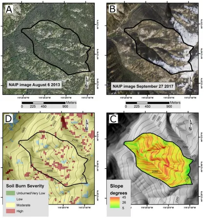
Figure 1.2: A) National Agricultural Image Program (NAIP) image of study site from 2013 (pre-fire). B) NAIP image of study site from 2017 (post-fire and post-debris-flow). C) Slope map of study area. 50 m contours for scale. D) Soil Burn Severity map from USFS Burned Area Emergency Response
(BAER). 50 m contours for scale. 11
Figure 1.3: A) Image of study catchment outlet post-fire and pre-debris-flow, taken from USFS helicopter. B) UAV image of debris-flow fan deposit. Orange rectangle marks approximate location of described and dated stratigraphy (Fig 4). C) Image of scoured channel from first visit to site, 9 days after debris-flow. Note mud lines, scarred trees and roots, and abrupt channel margins. D) UAV image of rilling on hillslope, arrows highlight individual
rills. 12
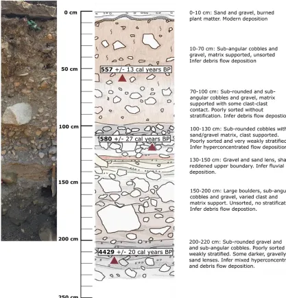
Figure 1.4: Fan deposit stratigraphy. Photo at left is 1 m upstream of described and dated section. At right, thicknesses and descriptions for units. Depths of dated charcoal fragments are shown by red triangles. In the field, we separated depths 10-130 cm into 3 units. Ages suggest they are from a single event. All deposits are fire-related except 130-150 cm depth. 14 Figure 1.5: Study catchment detail. More detailed hillshade shows extent of
SfM-derived 5 cm DEM. Green triangle is location of described and dated stratigraphic section (Fig 4). Black squares are locations of manually-surveyed channel cross-sections. Purple circles are locations of hillslope transects (n=15) scaled by the relative magnitude of rill erosion at each. Transects sample a range of slopes (14-37 degrees) and a variety of landscape positions. Blue diamonds mark channel head locations mapped in the field. 20 m contours shown for scale. 17 Figure 1.6: SfM methods and error assessment. A) Perspective view of point cloud
xiii
cloud compared to 20 RTK-GPS surveyed GCPs. A mix of positive (orange-red) and negative (blue-green) vertical errors indicates little
systematic distortion of the analyzed DEM. 21
Figure 1.7: A) UAV detail image of channel eroded by debris-flow. Orange boxes are in same location to aid comparison. B) 10 cm contour intervals highlight abrupt channel margin. C) Synthetic, pre-erosion surface created by removing “scour” points. D) Diagram of assumption correcting total calculated volume for a generic, pre-erosion geometry. E) Point cloud perspective view of same channel segment, showing detailed topographic
form and appearance of SfM point cloud. 23
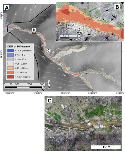
Figure 1.8: A) DEM of Difference for debris-flow channel scour. Red values indicate erosion and blue values indicate deposition. SfM topography extent is shown as hillshade. 20 m contour interval for scale. B) Detail of DoD corresponding to Figure 1.7. C) UAV image of section of channel scoured to bedrock by debris-flow. Flow is from right to left in all panels. 28 Figure 1.9: Upper left, Boxplots of rill dimensions from full dataset (n=175) and rill
counts per transect (n=15). Upper right, Monte Carlo simulation results showing variation in mean rill count per transect. Lower left, Monte Carlo simulation results showing variation in mean rill width (red) and depth (blue) dimensions. Lower right, Mean rill depth plotted against mean rill width, with linear best fit shown, note x and y axis scales. 31 Figure 1.10: Upper left, Boxplots of rill dimensions separated by aspect, and boxplots
of mean rill count per transect separated by aspect. Upper right: Monte Carlo results showing variation in mean rill counts on north aspects (blue) and South aspects (red). Lower left, S aspect mean rill counts plotted against N aspect mean rill counts, note x and y axis scales. While not statistically significant, north aspects had about three times as many rills as South aspects. Lower middle, Monte Carlo results showing variation in rill width and depth, separated by north aspect (blue) and South aspect (red). Lower right: Mean rill depth plotted against mean rill width, separated by north aspect (blue) and South aspect (red). Linear best fits
shown in black, note x and y axis scales. 41
0.1-xiv
Figure 1.12: Plot of erosion rates versus timescale of measurement from selected studies in discussion. Open symbols are data from Idaho, including this study shown in red. Closed symbols are from SW USA. Measurements of erosion rates are from a variety of methods and catchment sizes. Adapted from Kirchner et al., 2001 and Orem and Pelletier, 2016. 47 Figure 2.1: A) Area map of 2016 Pioneer Fire perimeter (orange) in Idaho. Yellow
circle is study catchment location Study catchment contributes to Clear Creek. B) UAS (aerial) image of rills on planar hillslopes connecting to scoured debris flow channel. Arrows give direction of flow. C) Detail map of study catchment. 0.95 km2 full extent outlined in gray. Extent of SfM 5 cm resolution DEM shown as hillshade. Red shading shows channel scour measured with DoD. Black triangles show locations of hillslope transect used to derive rill erosion volumes. Analyzed sub-basins are outlined. Labels at sub-basin outlets correspond to Table 2.1. 50 m contours for
scale. 55
Figure 2.2: Eroded volumes from sub-basins within study catchment. Channel eroded volume surpasses hillslope eroded volume at a drainage area of about 20 hectares (0.2 km2). Channel erosion volumes also increase about three times faster than rill erosion volumes, reflecting increased integration and efficiency of channel networks. Total erosion volume (channel + rill) is shown in gray squares. Rill erosion volumes (triangles) are extrapolated from hillslope transect data and applied as a uniform 1.4 mm per unit area erosion where rilling was observed. Channel erosion volumes (X’s) are from 5 cm resolution DEM of Difference derived from synthetic pre-erosion and surveyed post-pre-erosion Structure from Motion survey. Orange circles are data from post-fire gully erosion, in similar Idaho Batholith
terrain (Istanbulluoglu et al., 2003). 61
Figure 2.3: Sediment yield, in metric tons per hectare per year (mass/area/time) for sub-basins of varying size within the study catchment. Sediment yields increase as the scale of analysis increases, up to the 95 hectare study catchment size. Data from all drainage areas are fit with a power law function (black dashed line). Channel networks are not present at the smallest drainage areas. As drainage area increases, hillslopes are more closely coupled to channels and connectivity improves, allowing increased sediment yields. Green symbols represent contributing areas below 20 ha, where rill erosion contributes a majority of total erosion. Blue symbols represent contributing areas above 20 ha, where channel erosion
xv
Sediment yields are converted from measured eroded volumes using a
bulk density of 1500 kg/m3. 62
Figure 2.4: Percent contribution of hillslope erosion (rilling) to total erosion for varying size sub-basins within the study catchment. At small drainage areas, erosion is entirely by hillslope erosion. As the drainage area increases and channels are present, the relative contribution of hillslope erosion diminishes. In this setting, the threshold between hillslope-process dominance and channel-process dominance (purple shading) occurs at a drainage area of about 20 hectares (0.2 km2). Data are fit with a power law
function (dashed line). 63
Figure 2.5: Post-fire erosion literature values for sediment yield plotted against basin size. Sediment yield (t/ha) decreases as drainage area increases. A
common explanation for this negative relationship is increased opportunities for sediment storage or deposition in larger catchments (Lane et al., 1997; Scott et al., 1998; Shakesby and Doerr, 2006;
Wagenbrenner and Robichaud, 2014). However, this result seems at odds with data from sub-basins within our study catchment (Figure 2.3). Open circle symbols are measurements from multiple methods where basin sizes were clearly reported. Filled red diamond symbols are measurements from high-resolution topography (HRT) methods, this study is shown with purple squares. The HRT data are fit with a power law function (dotted
line). 71
Figure 2.6: Conceptual diagram from Swanson (1981) illustrating the intermittent
nature of post-fire sediment yields. 72
Figure 2.7: Post-fire literature values for the percent contribution of hillslope erosion to total erosion for varying basin sizes. At small drainage areas, hillslope processes contribute all or most erosion. As drainage area increases, channel processes become more dominant. Open circle symbols are measurements from multiple settings and methods where basin sizes were clearly reported. These data are fit with a power law function (black dashed line). Filled green triangle symbols are from high-resolution topography (HRT) methods, including this study shown with purple squares. HRT data are fit with a power law function (green dashed line). While taken from few data points, the similarity of fitted lines is
encouraging. Variation in the literature values is reflective of diverse settings (geology, fire, precipitation, basin characteristics, etc) as well as
PARTITIONED BY PROCESS: MEASURING POST-FIRE DEBRIS FLOW AND RILL EROSION WITH STRUCTURE FROM MOTION PHOTOGRAMMETRY
Chapter under review for publication in Earth Surface Processes and Landforms
Abstract
map and quantify channel erosion. We found 3467 ± 422 m3 was eroded by debris-flow scour. Rill dimensions along hillslope transects and Monte Carlo simulation show rilling eroded ~1100 m3 of sediment and define a volume uncertainty of 29%. The total eroded volume (4600 ± 740 m3) we measured in our study catchment is partitioned into 75% channel erosion and 25% rill erosion, reinforcing the importance of catchment size on erosion process-dominance. The deposit volume from the 2016 event was 5700 ± 1140 m3, indicating ~60% contribution from post-fire channel erosion. Dating of charcoal
fragments preserved in stratigraphy at the catchment outlet, and reconstructions of prior deposit volumes provide a record of Holocene fire-related debris-flows at this site; results suggest that episodic wildfire-driven erosion (~6 mm/year) dominate millennial-scale erosion (~5 mm/Ka) at this site.
Introduction
Modern post-fire erosion demands attention. Anthropogenic climate change is exacerbating the size and severity of wildfires, leading to dramatic impacts on
landscapes, ecosystems, human interests, and infrastructure (Goode et al., 2012; Abatzoglou et al., 2016; Sankey et al., 2017; Murphy et al., 2018). Pervasive post-fire erosion across steep landscapes exceeds background erosion rates by water-, gravity-, and wind-driven processes (Roering and Gerber, 2005; Shakesby and Doerr, 2006; Sankey et al., 2009; Moody et al., 2013). Hillslope and channel erosion processes interact with precipitation on steep, burned landscapes to produce and augment dramatic runoff-generated debris-flows (e.g. Meyer and Wells, 1997; Cannon et al., 2001; Gabet and Bookter, 2008). Runoff-generated debris-flows usually result from intense, convective precipitation in steep catchments, scouring channels and delivering large magnitudes of poorly-sorted sediment.
The occurrence and impacts of post-fire debris-flows are well documented (e.g. Cannon et al., 2010; Kean et al., 2011; Nyman et al., 2011), but questions remain about the relative contributions of hillslope and channel erosion to total sediment yield at various basin scales. In a range of basin sizes across the western United States, traditional surveying methods indicate post-fire channel erosion exceeds that from hillslopes (Santi et al., 2008; Moody and Martin, 2009). Hillslope processes, such as rilling, are difficult to measure across a landscape because they have small dimensions and are spatially
Benavides-Solorio and MacDonald, 2005; Pierson et al., 2009). However, plot-scale studies may miss the landscape-wide picture of erosion. Therefore, improving rill volume quantification, and its uncertainty, is required to more fully elucidate post-fire erosion processes.
Other recent work seeks to quantify the process-based erosion contributions using cm-resolution topography (e.g. terrestrial laser scanning, TLS) and multi-temporal change detection (e.g. DEM of Difference, DoD); several studies demonstrate that extensive hillslope erosion surpasses channel contributions (Staley et al., 2014; Rengers et al., 2016; Delong et al., 2018). Staley et al. (2014) show that >80% of post-fire erosion is from hillslopes and note that more work is needed at a range of catchment scales to determine when and how channel erosion exceeds hillslope erosion.
TLS surveys achieve cm-resolution, capture small landscape details, and reveal the spatial fingerprints and magnitudes of post-fire erosion processes, but are limited by viewing angle, occlusion, and scan locations across larger scales and in rugged settings. These studies are focused on relatively small areas (a few hectares) where significant post-fire erosion is anticipated. Further, they usually depend on collecting topographic data with lidar prior to precipitation; possible in certain situations but not feasible everywhere. Structure from Motion, Multi View Stereo photogrammetry (simplified to SfM hereafter) represents a lower-cost, flexible alternative to acquire cm-resolution topographic data (Johnson et al., 2014).
lidar, SfM point clouds are often gridded into DEMs during analysis. Many applications demonstrate SfM’s flexibility including investigations of shallow river topography (Javernick et al., 2014), coral reef roughness (Leon et al., 2015), landslide monitoring (Stumpf et al., 2015), and dryland vegetation (Cunliffe et al., 2016). James and Robson (2014) and James et al. (2017) give encompassing discussions and provide suggestions to minimize SfM error including high-quality imagery with some convergent geometries, adequate spatial coverage of ground control points (GCPs), and the inclusion of GCP uncertainty in models. SfM has proven to be enormously flexible with accuracy and resolution comparable to TLS. Furthermore, coupling SfM techniques with an unmanned aerial vehicle (UAV) platform makes this technology viable for quantifying post-fire erosion over rough terrain at suitable extents and cm-resolutions
The majority of post-fire studies have temporal scopes restricted to the present or a few decades prior, and limited work has been done on post-fire erosion over Holocene and Quaternary timescales (Moody et al., 2013; Murphy et al., 2018). A handful of studies investigate erosion and sedimentation responses to wildfire driven by Holocene climate changes by dating charcoal fragments from alluvial fans (Meyer and Pierce, 2003; Pierce et al., 2004, 2011; Bigio et al., 2010; Nelson and Pierce, 2010; Weppner et al., 2013; Riley et al., 2015; Fitch and Meyer, 2016). Over Quaternary timescales, post-fire erosion is responsible for >90% of landscape denudation since 1.24 Ma at Valles Caldera, New Mexico (Orem and Pelletier, 2016).
of rill erosion with high-resolution topography allows critical insights into the contributions of hillslope and channel processes to runoff-generated post-fire debris-flows.
Several primary research questions motivate this study: 1) How is channel and hillslope rill erosion partitioned following wildfire in a 1 km2 Idaho Batholith catchment? 2) How can estimates of rill erosion, and their uncertainty, be improved? 3) In the
absence of detailed pre-erosion topographic data, can SfM be used to map and quantify channel scour by runoff-generated debris-flow? A further goal of this study is to compare modern post-fire erosion with erosion over Holocene timescales. We apply cm-resolution SfM, traditional field work, and Monte Carlo simulation to quantify channel and rill eroded volumes and their uncertainties. We estimate paleo sediment yields at this site using radiocarbon dating of prior deposits. We then compare the Holocene values to observed modern post-fire erosion and to the results of similar studies.
Study Site
We studied a catchment within the ~35,000 km2 Idaho Batholith in central Idaho which burned in the 2016 Pioneer Fire (Figure 1.1A). The Pioneer Fire began in July 2016 and burned ~750 km2 of mountainous terrain on the Boise National Forest.Our
Over 80% (120 km2) of the Clear Creek drainage was burned at varying intensities in the Pioneer Fire (Burned Area Emergency Response
https://fsapps.nwcg.gov/afm/baer/download.php?year=2016, accessed October 2016). The study catchment was burned around August 30, 2016 at moderate to high severities (Figure 1.2).
The study catchment is 0.95 km2 in size, oriented approximately E-W, with elevations between 1778-2323 m. Mean catchment slopes are 26.2 degrees with a maximum of 45 degrees within the study catchment (Figure 1.2). Slopes are mostly soil-mantled with shallower, rockier soils and more bedrock outcrops on south aspects than north aspects. Latest-Pleistocene glacial features are present nearby in valleys above 2250 m elevation (Kiilsgaard et al., 2006), but mapped Quaternary deposits at the study
catchment are limited to low stream terraces and fan gravel. The study catchment is underlain by biotite-granodiorite intruded approximately 75 Ma (Kiilsgaard et al., 2006) with sparse Eocene rhyolite and dacite dikes. The catchment was last logged in the late 1950’s or early 1960s (D. Brown, personal communication, 2018). Most still-standing, burned trees have trunks <1 m diameter. Remnants of several skid roads are apparent on hillslopes.
October 2016 Precipitation and Debris-flow Events
hourly resolution) recorded maximum precipitation of 5 mm/hr and 8 mm/hr,
respectively. For reference, the 2-year recurrence interval precipitation at this location is 61.2 mm in 24 hours (http://www.nws.noaa.gov/ohd/hdsc/noaaatlas2.html, accessed September 2018) and the estimated October 15, 2016 precipitation was 25 mm in 24 hours (http://prism.oregonstate.edu/explorer/, accessed September 2018). The complex topography surrounding our study site modifies, and likely enhances, the precipitation produced by frontal-type storms (e.g. Daly et al., 1994; Mock, 1996). High-temporal resolution precipitation data are not available within 4 km of the study site (Staley et al., 2016, 2017), and therefore we do not attempt to report specific forcing data (peak 15-minute intensity) for the studied debris-flow.
Our study catchment was the only basin to produce a debris-flow within the Clear Creek drainage, as determined from reconnaissance along the entirety of Clear Creek using road access in October 2016 and June 2017. Indeed, little evidence of fresh depositional response was noted at any other catchment outlets. While this is surprising given the burn severity, the lack of response from nearby basins results from the modest precipitation intensity from the October 15, 2016 storm. Other steep basins along the axial South Fork Payette did produce fire-related debris-flows, resulting in large sediment and wood inputs, and rearrangement of rapids on this recreationally popular river.
15-minute rainfall intensity and 67% under 20 mm/hr peak 15-15-minute intensity
(https://landslides.usgs.gov/hazards/postfire_debrisflow/detail.php?objectid=5, accessed October 2016). In all, 20 basins within the Clear Creek drainage have probabilities exceeding 45% at 16 mm/hr rainfall intensity (Figure 1.1B). These 20 basins have
drainage areas ranging from 0.04 to 1.1 km2 and the predicted debris-flow volumes range from 389 to 10751 m3.
Our preliminary visit to the study site was on October 24, 2016, 9 days after the debris-flow. We were not able to conduct extensive field work at this time, but we made observations of the debris fan deposit and the lower section of channel. Clear Creek had already incised through the debris fan and carried some material downstream. Ash and charred organic matter were several centimeters thick upstream of the debris fan and in local depressions, indicating some redistribution and ponding post debris-flow. Ash was present on nearly all surfaces except where fresh sediment was exposed or deposited (i.e. channel and fan). Woody debris ranging from small branches to large trunks was
present up to 3 m above the freshly-scoured channel bed. We did not make observations of the upper channel reaches or much of the hillslopes during this preliminary visit.
Figure 1.1: A) geographic setting within Idaho, USA. Orange outline is extent of
2016 Pioneer Fire. B) USGS Post-Fire Debris-flow Hazard model results for
Figure 1.2: A) National Agricultural Image Program (NAIP) image of study site
Figure 1.3: A) Image of study catchment outlet post-fire and pre-debris-flow, taken from USFS helicopter. B) UAV image of debris-flow fan deposit. Orange rectangle marks approximate location of described and dated stratigraphy (Fig 4). C) Image of scoured channel from first visit to site, 9 days after debris-flow. Note mud lines, scarred trees and roots, and abrupt channel margins. D) UAV image of rilling on hillslope, arrows highlight individual rills.
Methods
Deposit Stratigraphy, Radiocarbon Ages, and Deposit Volumes
present is 1950) using OxCal v4.3.2 and the IntCal13 atmospheric curve (Reimer et al., 2013). Calibrated age ranges are reported at 95% confidence (2-sigma).
We estimated the deposit volume from the 2016 post-fire debris-flow and compared it to separate measurements of channel debris-flow scour and hillslope rill erosion. The eroded volume methods are described in subsequent sections. We also estimated the volume of previous debris-flow deposits preserved in alluvial fan
stratigraphy at the catchment outlet. We estimated the modern deposit volume, including portions removed downstream, using the extent of the deposit mapped from orthorectified UAV images, 12 measured depths where deposits were exposed, and 10 estimated depths where we judged deposition to have occurred but later removed downstream by spring runoff in Clear Creek. We created an interpolated surface from the measured and
estimated depths using inverse distance weighting (IDW) with a 0.5 m resolution grid of the mapped deposit extent, then summed the grid cell volumes for a total volume of the modern deposit. IDW was selected for interpolation by visual inspection of the results; it provided deposit depths that were representative of debris-flow and alluvial fan
deposition.
debris-flow dominated fans, but at this site we consider it an acceptable, first order approximation of paleo deposit volumes.
Figure 1.4: Fan deposit stratigraphy. Photo at left is 1 m upstream of described
Erosion Rates and Sediment Yields
We converted our deposit volumes to sediment yield (mass/area) and catchment-averaged erosion rate (depth/time) to allow comparisons with other post-fire erosion studies. We determined a catchment-averaged erosion rate (mm/Ka or mm/year) by dividing the deposit volume by the catchment area and the associated age. We propagated the 20% deposit volume error and the calibrated 2-sigma age ranges when calculating the catchment-averaged erosion rates. We converted our deposit volumes to sediment yield, in t/ha, using a bulk density of 1500 kg/m3 and the catchment area (Kirchner et al., 2001; Meyer et al., 2001). There are potential bulk density changes between eroded material and deposits, so the assumed bulk density of 1500 kg/m3 should be considered a tool for comparison and not necessarily as an absolute conversion from volume to mass.
Furthermore, the erosion rates and sediment yields we calculated represent minimum values because they pertain only to deposits preserved at one site on the alluvial fan. Hillslopes and Rill Eroded Volume
We did not explicitly measure interrill erosion but noted and observed
We used the rill dimensions recorded along hillslope transects and Monte Carlo simulation to quantify the volume of sediment eroded by rilling in the entire catchment. This approach requires two assumptions: 1) our transects sufficiently represent the variability in rilling across the catchment; and 2) the mean rill dimensions and counts come from an underlying normal distribution. Eighty percent of the paired width and depth values from the individual rills (n=175) were randomly sampled in Matlab and the variation in the means were calculated using 1000 Monte Carlo simulations. We also randomly sampled 10 of 15 transects and calculated the variation in mean count (number of rills per 20 m transect) using 1000 Monte Carlo simulations. From these simulations, we calculated a total cross-sectional area eroded by rilling per 20 m transect by
simplify the measured rill eroded volume by considering it to represent one full year of erosion.
Figure 1.5: Study catchment detail. More detailed hillshade shows extent of
SfM-derived 5 cm DEM. Green triangle is location of described and dated stratigraphic section (Fig 4). Black squares are locations of manually-surveyed channel cross-sections. Purple circles are locations of hillslope transects (n=15) scaled by the relative magnitude of rill erosion at each. Transects sample a range of slopes (14-37 degrees) and a variety of landscape positions. Blue diamonds mark channel head locations mapped in the field. 20 m contours shown for scale.
Calculation of Minimum Channel Erosion Volume
cited by others to this minimum eroded volume (e.g. Meyer et al., 2001; Santi et al., 2008; Moody and Martin, 2009). We also used the manual channel cross-sections to help assess error within the SfM model.
Structure from Motion Methods
While the manual channel cross-sections provide a minimum estimate of channel erosion, we sought to derive more explicit spatial information about the landscape and erosion processes by collecting high-resolution topography. We chose to apply UAV-based SfM to derive cm-resolution topography of the eroded channel in our steep, 1 km2 study catchment. After snowmelt in June 2017, we installed rebar (n=20) in stable and distributed hillslope and channel locations to serve as GCPs and recorded their locations with a TopCon HiperV real-time kinematic global positioning system (RTK-GPS). Points were post-processed to 0.01 m accuracy (https://www.ngs.noaa.gov/OPUS/, accessed September 2017) (Table 1). Orange bucket lids with centered holes were placed over each GCP rebar to serve as visual targets in UAV imagery. We conducted a total of 6 flights with a DJI Phantom 4 Pro UAV, covering 0.1 km2 of the debris-flow fan deposit, the primary channel, and the main tributaries with overlapping 20 megapixel images (Figure 1.6). Camera focus was automatic and focal length was fixed, while image
We used AgiSoft Photoscan Pro (http://www.agisoft.com/) to process the images into a point cloud and assign absolute locations of the GCPs projected to Universal Transverse Mercator Zone 11 North. The raw point cloud had 122 million points, each with an x,y,z position and a r,g,b value. The UAV images, original point cloud, and derived DEM are available on OpenTopography
(http://opentopo.sdsc.edu/dataspace/dataset?opentopoID=OTDS.012019.32611.1). We used CloudCompare (https://www.danielgm.net/cc/) for further analyses of the point cloud and to create DEMs. We cleaned the point cloud by manually removing noise points and those >1 m above the surface. Next, we subsampled the point cloud using 2.5 cm minimum spacing between points (62 million points remaining) and created a 5 cm resolution DEM of the post-erosion topography.
Table 1.1: Summary of ground control points (GCPs), their RTK-GPS accuracy,
and Agisoft-processed SfM root-mean-square error (RMSE). The 0.076 m (7.6 cm) total error includes all 20 available GCPs. For our SfM error analysis and volume uncertainty scenario 2 we randomly selected 10 GCPs to serve as control points, calculated the error, and repeated 3 times, resulting in 6.6 cm overall RMSE.
Ground control point name RTK-GPS horz accurac y (m) RTK-GPS vert accurac y (m) GCP accurac y carried into Agisoft (m) Error (m) X error (m) Y error (m) Z error (m)
119 0.004 0.008 0.008 0.0631 0.0509 0.0040 0.0372 123 0.004 0.005 0.005 0.0034 -0.0026 -0.0021 -0.0004 124 0.004 0.006 0.006 0.0077 0.0072 0.0023 0.0013 125 0.006 0.009 0.009 0.0191 -0.0184 0.0043 0.0029 126 0.004 0.009 0.009 0.0495 0.0169 0.0343 -0.0314 127 0.004 0.009 0.008 0.0201 0.0053 -0.0160 0.0110 128 0.004 0.008 0.008 0.0218 0.0181 0.0110 0.0054 129 0.004 0.008 0.008 0.0320 -0.0172 -0.0244 -0.0117 130 0.004 0.008 0.008 0.0172 -0.0068 0.0121 0.0102 131 0.003 0.006 0.006 0.0856 0.0195 -0.0559 0.0618 132 0.004 0.007 0.007 0.1065 -0.0765 -0.0526 0.0521 133 0.003 0.007 0.007 0.1077 -0.0619 -0.0877 0.0086 134 0.004 0.008 0.008 0.1375 -0.0817 -0.1103 -0.0082 135 0.003 0.007 0.007 0.1225 -0.0388 -0.1014 -0.0567 Total
error, m
0.0761 0.0444 0.0544 0.0294
Standard deviation of error, m
High-resolution pre-erosion topographic data was not available for our study site, but we needed a pre-erosion surface upon which to detect change and make calculations of channel eroded volume via a DEM of Difference (DoD) method. We obtained a DEM of the pre-erosion topography by removing the eroded portions and creating a synthetic surface derived from the surveyed, post-erosion point cloud (Figure 1.7A-E). We used the prominent, rectangular signature of debris-flow scour as a guide when removing eroded portions. In CloudCompare, we calculated contour lines at 10 cm intervals to highlight the abrupt scour margins (Figure 1.7B). We used the contours, in conjunction with the color and form of the SfM-derived point cloud, to manually remove scoured points. We fit a surface to the remaining non-scoured points using Delaunay triangulation (Figure 1.7C), enabling us to create a 5 cm resolution DEM of the synthetic, pre-erosion surface. Outside of the scoured channel the synthetic, pre-erosion point cloud and the SfM-derived, post-erosion point cloud are identical.
We created a DEM of Difference (DoD) to measure the volume of sediment eroded from the channel by debris-flow scour. We used Geomorphic Change Detection v7.3 software (Wheaton et al., 2010; http://gcd.riverscapes.xyz/) to compute the volume of erosion and incorporate our SfM volume error. All calculations were done using 5 cm resolution DEMs which we ensured were concurrent and orthogonal (Passalacqua et al., 2015). The GCD program incorporates user-specified error surfaces to calculate the DoD and outputs values of erosion or deposition for each grid cell, as well as tabular and graphical summaries. We did not incorporate spatially-variable error estimates
To account for a more realistic pre-erosion valley bottom we subtracted 25% from our calculated volume. This assumption is simple but subtracting a triangle (25%) from the rectangular channel cross-section mimics a generic pre-erosion valley geometry (Figure 1.7D). Similar approaches have been used (i.e. Meyer et al., 2001; Istanbulluoglu et al., 2003; Gabet and Bookter, 2008; Gartner et al., 2008; Santi et al., 2008; Nyman et al., 2015) when estimating the pre-erosion geometry of gullies. The volume of channel erosion we measured in Summer 2017 is primarily from the October 2016 debris-flow but may also include minor erosion during snowmelt. We simplify the measured channel eroded volume by considering it to represent one full year of erosion.
Figure 1.7: A) UAV detail image of channel eroded by debris-flow. Orange boxes
Structure from Motion Error Analysis
We used 2 approaches to assess error within our SfM model. First, we calculated the vertical root mean square error (RMSE) and mean average error (MAE) between manual channel cross-sections (n=4) and corresponding topographic profiles extracted from the point cloud (z-coord only). We ignored measurement error within the manual channel cross-sections. There is also the possibility of slight misalignment of the SfM point cloud coordinates with the local coordinate system used for the manual cross-sections. In our second approach, we considered the maximum error in horizontal (x,y coord) or vertical (z-coord) directions from the post-processed RTK-GPS ground control points and carried these into the SfM model. Using a random number generator, we chose 10 out of the available 20 GCPs to serve as check points. We calculated the RMSE (x,y,z coords) between the RTK-GPS GCP locations and the SfM model GCP locations, then averaged the results of 3 trials. The resulting overall RMSE accounts for both the RTK-GPS error and the SfM model error in all three dimensions.
created from the same SfM model and therefore share the exact same reference system, ground control points, extents, resolution, and accuracy. When comparing other high-resolution topographic datasets (e.g. TLS post- to Airborne Laser Scanning (ALS) pre-), there can be significant uncertainty due to instrument error, georeferencing, and gridding operations (e.g. Delong et al., 2012). In our situation, the pre-erosion and post-erosion DEMs are derived from the same point cloud and propagating the error from just the pre-erosion DEM is supported. In the final scenario we calculated a probabilistic error budget (0.8 confidence level) using 10 cm spatially uniform error for the surveyed, post-erosion topography and no error (0 cm) for the synthetic, pre-erosion topography. We chose 10 cm to split the difference between the first scenario, which we consider
overly-conservative, and the second scenario, which is a minimum representation of error. Using this final scenario, error was 12% of the calculated volume. Based on our analyses we judged this final scenario to be the most suitable error budget and use it for subsequent results and interpretations.
produce a satisfactory ‘bare-earth’ DEM at comparable resolution upon which to detect changes from the 2017 survey.
Results
Channel Erosion
The volume eroded from the channel by debris-flow scour was 3467 ± 422 m3 as derived from the DoD approach (Table 2). This represents ~75% of the total measured eroded volume (debris-flow + rills) or ~60% of the estimated deposit volume. The DoD change detection map reveals spatial variations in erosion at 5 cm resolution; the greatest scour depths occur downstream of bedrock knickpoints (Figure 1.8). Mean scour depth was 0.8 m and 77% of scour depths were between 0.25 and 1.5 m. The SfM survey did not extend to channel heads but we visited those locations in the field (Figure 1.5). The rectangular cross-section of the scoured channel persisted during our field work and cut into fresh bedrock in some reaches. We observed debris-flow signatures such as scarred trunks and clasts up to 0.5 m diameter deposited upstream of channel constrictions and obstructions in the upper reaches. We also observed small bank collapses and
Table 1.2: Summary of eroded volumes and uncertainties. Values in bold used for analysis and discussion
Method/scenario Volume
eroded (m3)
Volume uncertainty (m3)
Volume uncertainty (%)
Channel erosion, manual cross-sections 3300 660 20% Channel erosion by DoD, scenario 1
(minimum LOD)
3453 655 19%
Channel erosion by DoD, scenario 2 (propagated error)
3485 298 8%
Channel erosion by DoD, scenario 3 (0.8 probabilistic error)
3467 422 12%
Rill erosion by Monte Carlo, lower 811 - -
Rill erosion by Monte Carlo, mean 1104 320 29%
Structure from Motion Error
Both approaches we used to determine SfM error fit closely with previous
assessments (Johnson et al., 2014; Lucieer et al., 2014). Mean SfM point cloud RMSE (z-coord) was 0.16 m (MAE 0.03 m) when compared to our manual channel cross-sections. SfM point cloud RMSE (x, y, z coords) was 0.076 m when compared to all 20 available RTK-GPS ground control points (Table 1) and 0.066 m using 3 trials of 10 random GCPs each.
Eroded Volumes from Hillslopes and Rills
(Figure 1.9). The rill dimension measurements and counts along our transects were not significantly correlated with slope or contributing area.
Deposit Stratigraphy, Radiocarbon Ages, and Deposit Volumes
Alluvial fan stratigraphic sequences at the study site outlet preserve ~4.5 Ka of fire-related deposition. At our sampling site where the stratigraphy was best exposed, we split the stratigraphic exposure into six units based on sedimentary characteristics and inferred depositional processes (Figure 1.4) and three dated charcoal fragments (Table 3). Samples 4-2 and 4-4 likely record the same fire-related debris-flow event at ~560 cal yr BP. Taken together with the stratigraphy and estimated deposit volumes, these ages indicate three significant fire-related debris-flow events every ~5 Ka and a recurrence interval (of deposition, not fire) of ~1.6 Ka. We acknowledge that there are likely depositional events preserved elsewhere on the alluvial fan that are not represented by our ages from the described stratigraphic section.
Table 1.3: Radiocarbon dates from charcoal fragments preserved in stratigraphy at study catchment outlet.
Sample name (lab sample number)
Sample depth (m)
14C age, year BP (1-sigma)
Calibrated age, year BP (2-sigma)
4-2 (X32824) 0.6 601 (18) 557 (13)
4-4 (X32826) 1.2 628 (19) 580 (27)
4-6 (X32825) 2.2 3970 (21) 4429 (20)
Erosion Rates and Sediment Yields
Table 1.4: Estimated deposit volumes and conversions to catchment-averaged sediment yield and erosion rate. The deposit volumes represent single events based on stratigraphy and radiocarbon ages. The sediment yield and erosion rate are calculate including overlying deposits to represent longer-term averages.
Deposit age Volume, m3 (uncertainty) Catchment-averaged sediment yield, t/ha/Ka (range) Catchment-averaged erosion, mm/Ka (range)
modern (*1-year) 5716 (1143) *90 (17) *6 (1)
~560 cal year BP 6300 (1260) 336 (80) 22 (6)
~4420 cal year BP 10000 (2000) 78 (16) 5 (1)
Discussion
Precipitation Characterization and Context for Debris-flow Prediction
Local specific forcing data and detailed pre- and post-erosion topography are desirable to link precipitation to erosion processes (e.g. DeLong et al., 2018). However, in a large fire with high erosion potential in many basins, the allocation of equipment and focus must be balanced with access and hazards. While it is possible to single out small areas where post-fire erosion is anticipated, catchments will not produce debris-flows after every fire, as evidenced by this site’s charcoal record and by the absence of other debris-flows within the Clear Creek drainage. We lack local, high temporal resolution precipitation data and we were not able to acquire pre-erosion topography; a common and realistic situation. We took advantage of debris-flow occurrence in this representative catchment by using the rich topographic information provided by SfM to investigate our research questions.
unknown, but from available hourly (~10mm/hr) and daily (~25 mm/24 hours) data we characterize the mesoscale precipitation from the October 2016 frontal storm as modest. That said, precipitation in mountainous areas can be highly spatially variable (e.g. Bales et al., 2006; Stratton et al., 2009), and given that this particular basin failed and adjacent similar basins did not, one possibility is this basin received higher rainfall. Brogan et al. (2017) report an environment where mesoscale precipitation resulted in greater
geomorphic change than convective precipitation via fluvial processes. However,
Benavides-Solorio and Macdonald (2005) found that convective storms produce >90% of hillslope plot erosion, and Kampf et al. (2016) found average sediment yields doubled in convective versus mesoscale storms. Hillslope erosion processes vary with precipitation intensities (McGuire et al., 2016), but linking the contribution of each hillslope process to debris-flows generated by runoff under a wider range of conditions remains an important topic. The October 2016 debris-flow triggered by modest rainfall at our study site serves as a reminder that post-fire hazards are not limited to especially high-intensity convective precipitation.
We used the USGS post-fire debris-flow hazard model to provide additional context for our results. Using our estimated 2016 deposit volume (5700 m3) as a
parameter, the peak 15-minute precipitation intensity predicted by the USGS model is ~13.5 mm/hr. The model predicts a 50% likelihood of debris-flow occurrence in our study basin under ~17 mm/hr peak 15-minute rainfall and predicts a volume of 6695 m3 (~17% greater than 2016 deposit volume). The total eroded volume we measured (4600 ± 740 m3) and total deposited volume that we estimated (5700 ± 1140 m3) fit the USGS
uncertainties. Further, the USGS model allows some quantitative characterization of the October 2016 event-triggering rainfall. At 16 mm/hr peak 15-minute rainfall (one of the design storm intensities used for preliminary assessment), the USGS model predicts 18 basins in the Clear Creek drainage to have higher probabilities of debris-flow occurrence than our study catchment. To date, ours is the only catchment in the Clear Creek basin that has produced a debris-flow. Eighty-five percent of runoff-generated debris-flows occur in the 1st year after fire, diminishing the likelihood of more debris-flows in the
Clear Creek basin (Degraff et al., 2015). We infer that debris-flow occurrence in our study catchment reflects factors not entirely captured by the current USGS post-fire debris-flow hazard model because many other nearby basins had equal or higher
probabilities but did not produce debris-flows under widespread but modest precipitation in October 2016. The study catchment produced a debris-flow ~600 years ago, so perhaps the time since the last channel-evacuating debris-flow, and accumulation of sediment on hillslopes and channels modifies the post-fire hazard in this setting.
Structure from Motion: Accuracy, Advantages, and Recommendations
SfM data to TLS data as a reference and found 2-20 cm error (Cook, 2017; Johnson et al., 2014; Stumpf et al., 2015). Johnson et al. (2014) also compared SfM to ALS data as a reference and found error was <13 cm for 90% of points. Gillan et al. (2017) compared UAV-derived SfM measurements to manual erosion bridge measurements along
topographic transects and calculated an RMSE of ~3 cm. Clapuyt et al. (2016) tested the reproducibility of SfM topographic datasets and found 6 cm MAE within their workflow. Our assessment of SfM error (16 cm using manual channel cross sections, 6.6 cm using RTK-GPS surveyed GCPs) fits closely with these studies and show that SfM is a viable, accurate method to quantify post-fire erosion volumes.
Continued work on georeferencing accuracy is critical to improving change detection using ultra-high resolution topography (e.g. Passalacqua et al., 2015; DeLong et al., 2018). Our results show that low error (6.6 cm) and very high spatial resolution (5 cm DEM) are possible when sub-centimeter RTK-GPS ground control is integrated into SfM surveys, even in a steep and challenging landscape. However, current SfM
GCP locations (Clapuyt et al., 2016). Regularizing UAV flight paths and image locations, as Goetz et al. (2018) have done, is an important methodological consideration for future change detection via SfM.
The ease of acquiring cm-resolution topography via UAV and SfM provided a logistic advantage over TLS at our study site. A comparable TLS point cloud extent would require many scan locations to accommodate the rugged topography and occlusion from standing burned trees. The orange bucket lids over rebar GCPs worked well for visibility in UAV imagery and in the field. In such a steep, rugged study site, setting up the GCP network and recording it with RTK-GPS took longer than executing the UAV flights. The directly georeferenced UAV-SfM options becoming available would have an advantage in particularly high-relief study sites (Carbonneau and Dietrich, 2017; Turner et al., 2014).
The regrowth of vegetation was significant 2 years post-fire, reducing the occurrence and magnitude of further erosion (i.e. Orem and Pelletier, 2015; Wagenbrenner and Robichaud, 2014). Additionally, the spatial coverage of new
vegetation on the landscape precludes the use of SfM to derive cm-resolution topographic models for change detection. We were not able to produce a satisfactory “bare earth” model from 2018 at an equivalent resolution as the 2017 survey. The limitations of SfM, namely vegetation and georeferencing, must be considered when applied to geomorphic change detection.
Post-Fire Erosion Processes
Dietrich, 2006). We did not observe any large colluvial failures as expected in a debris-flow triggered by saturation failure (i.e. Costa, 1984; Stock and Dietrich, 2006). Instead, widespread rilling and inferred extensive overland flow led to a runoff-generated debris-flow (e.g. Meyer and Wells, 1997; Cannon et al., 2001; Gabet and Bookter, 2008). As Kean et al. (2013) and Rengers et al. (2017) show, runoff-generated debris-flow initiation often requires sediment to be introduced to the channel, temporarily stored, and then fail. It was difficult to pinpoint specific initiation points in the field, but markers
representative of debris-flows including small levees, inset deposits of large-caliber clasts, and scarred vegetation were present throughout the SfM-surveyed channel sections and >75% of the distance to channel heads. Widespread hillslope rilling, and inferred interrill erosion, provided the in-channel sediment necessary for debris-flow initiation.
The range in sample means also defines the 29% volume uncertainty in our approach; a clear advantage over prior work that does not report uncertainty. Finally, Monte Carlo simulation highlights the difference between rilling on north and south aspects (Figure 1.10). Fitch and Meyer (2016) found north-facing basins experienced more post-fire erosion in the late-Holocene based on analyses of alluvial fan stratigraphy in the Jemez Mountains, but they do not split it into specific process differences. While not statistically significant, the north-facing aspects exhibit more numerous rills with smaller dimensions than the south-facing aspects. We attribute this difference to generally finer-grained regolith on north aspects as noted in the field, but further exploration is warranted. Rilling was not significantly correlated with slope, perhaps an effect of only making 15 transects and extracting their slopes from 10 m resolution elevation data. Moody and Martin (2009) report an “inability to link slopes to actual erosion sites” and did not correlate sediment yield with slope. Similarly, Perreault et al. (2017) found no strong correlations between terrain attributes (such as slope) and diffusive hillslope erosion and suggested that stochasticity may obscure predicted relationships.
Figure 1.10: Upper left, Boxplots of rill dimensions separated by aspect, and boxplots of mean rill count per transect separated by aspect. Upper right: Monte Carlo results showing variation in mean rill counts on north aspects (blue) and South aspects (red). Lower left, S aspect mean rill counts plotted against N aspect mean rill counts, note x and y axis scales. While not statistically significant, north aspects had about three times as many rills as South aspects. Lower middle, Monte Carlo results showing variation in rill width and depth, separated by north aspect (blue) and South aspect (red). Lower right: Mean rill depth plotted against mean rill width, separated by north aspect (blue) and South aspect (red). Linear best fits shown in black, note x and y axis scales.
Partitioning of Erosion Processes
their review, Moody and Martin (2009) report a factor of 3 greater sediment eroded from channels than from hillslopes in the year following fire (240 t/ha vs 82 t/ha). Conversely, multiple TLS studies show hillslope erosion exceeds channel erosion (DeLong et al., 2018; Rengers et al., 2016; Staley et al., 2014). Rengers et al. (2016) found erosion from hillslopes was 3 times greater than from convergent, incipient channels at a 0.55 ha study site in Colorado. Staley et al. (2014) determined ~80% of total erosion came from
hillslopes with contributing areas <40 m2 in Southern California. In Arizona, overland
flow and rilling produced 68% of total post-fire erosion while channels produced 32% (DeLong et al., 2018). Nyman et al. (2015) calculated ~50% of total erosion was
drainage areas (a few sq km) and subsequently channel erosion processes dominate total erosion. Other studies have examined relationships between drainage area and erosional processes (e.g. Montgomery and Foufoula-Georgiou, 1993; Moody and Kinner, 2006; Reneau et al., 2007; Scott et al., 1998; Stock and Dietrich, 2006; Wagenbrenner and Robichaud, 2014). However, more work is needed to 1) examine how fire alters relationships between erosional processes and drainage area, and 2) integrate high-resolution topography into a wider range of drainage areas.
Our measured volume of erosion (debris-flow + rills) was ~4600 (± 740) m3 while our estimated deposit volume was 5700 (± 1140) m3. The eroded and deposited volumes overlap within error. However, we noted widespread evidence of interrill hillslope erosion. Several possibilities exist: 1) “missing” portion of deposit volume (~1100 m3, or
Figure 1.11: Comparison of post-fire studies reporting contribution from channel erosion processes to total erosion. Channel processes include debris-flow,
hyperconcentrated flow, and streamflow. Solid columns are from high-resolution topography and single catchments. Hollow columns are from other methods or
averages from multiple catchments. Catchment sizes are 0.075 km2 (Delong), 0.5
km2 (Meyer), various (Moody and Martin), 0.1-2.2 km2 (Nyman), 0.005 km2
(Rengers), 0.5-5 km2 (Santi), 0.07-0.2 km2 (Smith), 0.01 km2 (Staley), and 0.95 km2
(this study).
Modern and Holocene Erosion Rate and Sediment Yield Comparison
Our basin produced a total sediment yield of 90 t/ha (from estimated deposit volume) in the first year after fire; 17 t/ha (from measured rill volume) came from rilling alone. Meyer et al. (2001) describe two nearby, ~0.5 km2 basins (one unburned) that
Sediment yields from hillslope erosion on burned plots in Colorado are 10-12 t/ha per year (Benavides-Solorio and MacDonald, 2005; Schmeer et al., 2018). The average value for post-fire hillslope erosion across the Western US is 82 t/ha/year (Moody and Martin, 2009). In a coarse-scale modeling study, Miller et al. (2011) predict 2 t/ha/year for hillslope erosion in the intermountain West; more than 7 times less than what we measured with rilling alone. Using the ~35,000 km2 Salmon River basin in Idaho as their domain, Gould et al. (2016) model an increase of 31 t/ha/year sediment yield under future climate scenarios linked to increases in fire frequency and severity. However, neither study includes mass wasting processes (debris-flows) in their models, which integrate over large watersheds and dominate the sediment yield and erosion rate over Ka timescales (Kirchner et al., 2001).
the role of each would require information on debris-flow magnitudes from a wider range of spatial and temporal settings.
We calculated 78 (± 16) t/ha/Ka for the sediment yield since ~4420 cal year BP and 90 (± 17) t/ha in the modern event. Put simply, the sediment yield from 2016 erosion alone more than satisfies the average sediment yield over the last 4.4 Ka at this site. Nearby, Meyer at al. (2001) found an average sediment yield of ~160 t/ha/Ka between 7.4 and 6.6 Ka from alluvial fan records; our modern yield accounts for >55% of that in a single event. Kirchner et al. (2001) calculated sediment yields and denudation rates for 32 basins in Idaho ranging from 0.2-35,000 km2 using 10Be concentrations in alluvial
sediments. Averaged over 5-27 Ka, sediment yields were 550-2600 t/ha/Ka and denudation rates were ~20-100 mm/Ka (Figure 1.12). Kirchner et al. (2001) compared their long-term values to measurements of sediment flux in streams and concluded that 70-97% of sediment is delivered in infrequent, large-magnitude events, i.e. extreme floods and following wildfire. Riley (2012) attributed 40-70% of the 35,000 km2 Salmon River basin sediment yield over the last 6 Ka to post-fire debris-flows in the tributary 7500 km2 Middle Fork Salmon River basin. Therefore, we argue that post-fire erosion, while brief and separated by long quiescent periods, dominates the long-term erosion signal in the Idaho Batholith and elsewhere.
year post-fire was 6 mm/yr, and our long-term rate was 5mm/Ka; the same order of magnitude as Orem and Pelletier’s (2016) estimates. In the Chiricahua Mountains in Arizona, 22 mm of catchment-averaged erosion in a 7.5 ha catchment from a 10-yr recurrence interval convective storm drastically exceeds the (not specifically fire-related) millennial-scale erosion rate of ~0.04 mm/yr from the nearby Pinaleno Mountains
(Jungers and Heimsath, 2016; DeLong et al., 2018). In addition to these examples, numerous modern studies have measured post-fire erosion rates and magnitudes that greatly exceed background erosion (e.g. Moody et al., 2013). Our study corroborates prior work describing the critical impact of post-fire erosion over Holocene and Quaternary timescales.
Conclusion
Hillslope and channel erosion processes interact to produce ubiquitous erosion after wildfire in steep terrain. However, measuring each process is difficult at the scale of a typical catchment and few studies include Holocene magnitudes of post-fire erosion.
This study presents methods for partitioning post-fire rill and channel erosion processes that are flexible and robust. Importantly, we show that insights into erosional processes, sediment volumes, and their uncertainties, can be made across a
AN ISSUE OF SCALE: CONTRIBUTING AREA AND POST-FIRE EROSION Abstract
At catchment outlets, the impacts of post-fire erosion on communities,
infrastructure, and ecosystems are being highlighted and augmented by climate change. In steep, burned catchments, sediment is mobilized from hillslopes by multiple erosional processes; the basin-scale post-fire erosional response is ultimately controlled by a complex combination of basin characteristics (e.g. slope angle), sediment availability, precipitation variables, and the interaction and integration of channel networks and hillslopes. We use a 0.95 km2 catchment burned in the 2016 Pioneer Fire in Idaho to quantify an important spatial threshold separating hillslope and channel erosion processes. Modest precipitation produced widespread rilling and a runoff-generated debris flow in the study catchment. We measure channel erosion by debris flow scour using 5 cm resolution Structure from Motion topography and hillslope erosion by rilling using transect data and explore their relationship at varying sub-basin sizes. We
document the decreasing importance of hillslope processes to total eroded volumes as drainage area increases. In this setting, there is approximate parity between hillslope and channel eroded volumes at a drainage area of 0.2 km2 (20 ha): channel erosion dominates
the overall signal for contributing areas greater than 0.2 km2 and hillslope erosion
from our study catchment to values from the post-fire literature, confirming the shift from hillslope-dominance to channel-dominance as drainage basin areas increases. Our sub-basin analyses show sediment yield increases with drainage area while other studies show the inverse, reflecting a variety of influences. Among these influences are the diverse geographic and geologic settings, the precipitation values, and the burn severity.
Furthermore, the selection of field sites, the mode of measurement, and the timescale of measurement affect the reported sediment yield to drainage area relationship.
Investigations into spatial thresholds separating hillslope and channel process-dominance, especially when coupled with high resolution topography, will help to quantify the
landscape reaction to wildfire in other settings. Introduction
Erosional processes in burned landscapes produce rapid and dramatic landscape changes which impact communities, infrastructure, and ecosystems. However, the
delivery of sediment from hillslopes to basin mouths, where most homes, roads and other infrastructure are located depends on the connectivity of hillslopes and channels.
Connectivity is a continuum representing how efficiently material is transferred between landscape components (Grant et al., 2017; Wohl et al., 2018). Connectivity includes two concepts that vary in time and space: structural connectivity and functional connectivity (Wohl et al., 2018). Functional connectivity refers to the processes
Significant work has been devoted to thresholds across many systems, including Schumm’s (1973) concept of complex response. For example, sediment flux is controlled by a critical gradient threshold (Roering et al., 1999), landscape dissection and channel initiation are controlled by a slope-area threshold (Montgomery and Dietrich, 1992; Montgomery and Foufoula-Georgiou, 1993), thresholds influence the occurrence of distinct hillslope processes (Dietrich et al., 1992), link river incision to tectonic uplift (Snyder et al., 2000), and couple hillslopes to valleys incised by derbis flows (Stock and Dietrich, 2006). The spatial threshold of 0.1-1 km2 drainage area signifies a transition to fluvial processes in many settings (Stock and Dietrich, 2006).
In post-fire settings, debris flows are initiated above a precipitation intensity-duration threshold or when a critical channel stability threshold is reached (McGuire et al., 2017; Staley et al., 2017). Wildfire changes infiltration, friction, and shear stress, reducing the critical area required for channel initiation or promoting infiltration-excess overland flow (Moody and Kinner, 2006; McGuire et al., 2018).
Fire usually reduces critical area, impacting hillslope processes (e.g. rilling, dry ravel, raindrop impact, and sheetwash) and their connectivity to channels (Meyer and Wells, 1997; Cannon et al., 2001; Moody and Kinner, 2006; Reneau et al., 2007; Moody et al., 2013). Hillslope erosional processes can promote debris flows when they transport material downslope and rapidly introduce sediment to channels (Staley et al., 2014). Therefore, high connectivity implies hillslopes and channels are closely coupled, allowing efficient export of detached sediment to the channel network, while low
threshold differentiating low-efficiency (primarily hillslope) erosion from high-efficiency (primarily channel) erosion for a particular post-fire landscape.
In recent decades, high resolution topography (HRT) has significantly enhanced our understanding of landscape change through its ability to detect connectivity pathways and quantify thresholds (Passalacqua et al., 2015; Wohl et al., 2018). We define HRT as having 1 m or finer spatial resolution (e.g. Airborne Laser Swath Mapping (ALSM), Terrestrial Laser Scanning (TLS), and Structure from Motion Multi View Stereo (SfM-MVS, simplified to SfM hereafter). Moody et al. (2013) call for quantitative metrics to describe post-fire erosion processes and thresholds. Here, we investigate one post-fire threshold using SfM-derived HRT and hillslope transects.
This study intends to evaluate how post-fire hillslope and channel erosion vary with drainage area. Specifically, we demonstrate the drainage area threshold separating dominantly hillslope erosion from dominantly channel erosion for a 0.95 km2 burned catchment in Idaho and relate it to connectivity. To do so, we produce and analyze a dataset of channel erosion by debris flow scour and hillslope erosion by rilling across multiple sub-basin sizes. Further, we ask how hillslope contributions to total erosion and sediment yield evolve with increasing drainage area, and we compare our observations to relevant literature.
Study Site, Debris Flow Occurrence, and Field Observations
Our study catchment is a 0.95 km2 headwater catchment burned at moderate to high intensities in the ~750 km2 2016 Pioneer Fire in Idaho, USA (Figure 2.1A). The study catchment ranges in elevation from 1770-2320 m with 26o average slopes (45o
Cretaceous biotite-granodiorite. Slopes are mostly soil-mantled and planar, becoming less steep near drainage divides. Valleys are v-shaped with a main channel and several
tributaries supporting ephemeral flow. Pre-fire vegetation included Douglas Fir
Figure 2.1: A) Area map of 2016 Pioneer Fire perimeter (orange) in Idaho. Yellow circle is study catchment location Study catchment contributes to Clear Creek. B) UAS (aerial) image of rills on planar hillslopes connecting to scoured debris flow
channel. Arrows give direction of flow. C) Detail map of study catchment. 0.95 km2
The catchment was burned around August 30, 2016. A debris flow was triggered on October 15, 2016 with the catchment receiving 25 mm of rain in 24 hours with an estimated peak 15-minute intensity of 10 mm/hr (http://prism.oregonstate.edu/explorer/, accessed September 2018; https://wcc.sc.egov.usda.gov/nwcc/site?sitenum=312,
accessed September 2018). Erosion response to this modest precipitation included widespread hillslope rilling leading to a runoff-generated debris flow. A large volume of sediment and large woody debris was delivered to the catchment outlet fan and impinged on Clear Creek.
Rilling was pervasive across the catchment, with rill heads located a few tens of meters from drainage divides. Rills on planar slopes were parallel and often
discontinuous with lengths 10-100 m (Figure 2.1B). Rills coalesced into shallow gullies where topography was convergent. Burned out root casts were common and provided conduits into the subsurface. Rills were more common in the finer-grained regolith of north facing slopes. Besides hillslope rilling, burn marks on rocks and pedestals below rootlets and pebbles indicated raindrop impact and sheetwash had removed surface material, and flakes were spalled from granite boulders.