Published online May 2, 2013 (http://www.sciencepublishinggroup.com/j/wcmc) doi: 10.11648/j.wcmc.20130101.12
The details of virtual contention window concept for
802.11 IBSS wireless local area network mathematic
modelling
Anton V. Lazebnyy
1111,
,
,
,
Volodymyr S. Lazebnyy
22221Scientific and Production Enterprise"Ukrservisbud" Ltd., Kyiv, Ukraine, systemadministrator, MA
2National Technical University of Ukraine "Kyiv Polytechnic Institute", Kyiv, Ukraine, Associate Professor, Ph.D. NTUU "KPI", Kyiv,
Ukraine
Email address:
[email protected] (V. S. Lazebnyy)
To cite this article:
Anton V. Lazebnyy, Volodymyr S. Lazebnyy. The Details of Virtual Contention Window Concept for 802.11 IBSS Wireless Local Area Network Mathematic Modeling. International Journal of Wireless Communications and Mobile Computing. Vol. 1, No. 1, 2013, pp. 7-13. doi: 10.11648/j.wcmc.20130101.12
Abstract:
The concept of a virtual contention window for assessment of temporal and probabilistic characteristics of the processes occurring in the wireless LAN 802.11 is considered. The relations for determining the transmission time delay of the data package, the uneven of transmission time, throughput of wireless channel, the probability of packet loss for networks with saturated load are proposed in this paper.Keywords:
Collision Probability, Contention Window, Jitter, Saturated Payload, Throughput of Wireless Channel, Time Delay, Wireless Network1. Introduction
The wireless local area networks (WLAN) of 802.11 [1] standard are widely use for privet nets on the one hand and corporative nets with large number of users on the other hand.
If we shall analyze the development of 802.11 standard during a time, we shall see different changes on physical and channel levels (802.11 a, b, g, n), which was done in order to improve some characteristics of local wireless telecommu-nication systems. In this paper we shall speak only about physical and channel levels of 802.11 standard.
Accordingly with 802.11 standard it may be two types of wireless networks: BSS - Basic Service Set and IBSS – Independent Basic Service Set.
In BSS mode all subscribers not connected directly but through AP (Access Point). Such a wireless network con-trolled by PCF (Point Coordination Function).
In IBSS mode all subscribers connected one to another directly by using CSMA/CA (Carrier Sense Multiple Ac-cess/Collision Avoidance) competitive access method and DCF (Distributed Coordination Function) will be used to control the communications.
If we use IBSS mode, we can get a most throughput in comparison with BSS mode but reliability of connections in
IBSS network will be less, because the competitive access method on physical channel will be used.
There are a lot of investigations and scientific works corresponded with analysis of processes and parameters of IBSS networks. Some books [2-12] contain fundamental principles of wireless 802.11 standard networks functioning analysis. There we can see the most of models proposed for wireless network description. It possible to estimate the accuracy of different models and it’s convenience on prac-tice. Some of these models [2] give us a general description of probable events on 802.11 wireless networks by using of integral expressions. Such expressions are not convenient on practice because they don’t give a direct dependence be-tween network parameters and it’s performance. Other models [3,4] based on the concept of saturated network load proposed by Giuseppe Bianchi. This models give ability to estimate the influence of system parameters on network performance but only in general and calculation may be done only for limited range of parameters. If we attentively look on one of such expression [3, formula (36)]:
) ) ( )( ( ) )(
(
) )(
(
1 1
1
2 1 1 1
2 1
1 2 1 2
+ +
+
− − + − −
− −
= R
c c
R c c
R c c
p p
W p
p
p p
τ , (1)
the meaning of collision probability pc must be less then 0,5,
because in the case of pc = 0,5 it will be «zero» in the
nu-merator of shown expression. The second singularity of considered expression corresponded with pc = 0. In this case
the probability of successful transmitting of data pocket τ will depends only by meaning of contention window W. Because W may be equal to 8, 16 or 32 corresponding with different specifications of 802.11 standard, the calculated meaning of successful transmitting will be significantly less then «one». Such result takes place because formula (1) was proposed for estimation of successful transmitting proba-bility for process, which has begun during some elementary time slot. That’s why it is difficult to use such a formula in order to execute an accurate analysis of processes, which take place in wireless networks.
Due to problems which are considered and some other problems many scientists make their efforts in order to im-prove approaches for wireless networks performance esti-mation.
2. The Concept of Virtual Contention
Window
It's well-known that in order to get access to wireless channel in Wi-Fi LAN every station use the parameter which named Contention Window (CW). This interval form by using the CW, the value of which is chosen randomly from the set of numbers {0,1,2, ..., CW}. CW defines the number of elementary timeslots which form the transmitting delay.
We propose to use the concept of saturated network load proposed by Giuseppe Bianchi [2] and consider the process of packets transmitting as a quasistationary process.
The main idea of the Virtual Contention Window concept is that in average every station of network will transmit its packets by equal time intervals, which we called the Virtual Contention Window.
Virtual Contention Window as a parameter VCW is a stochastic parameter of unplanned wireless network stan-dard 802.11 (BSS), which is numerically equal to the aver-aged number of elementary time intervals (time slots) during which the backoff counter provides a delay interval after transmitting the previous frame before transmitting the next data frame of one station.
Duration of time interval corresponding to the virtual contention window depends on the number of active stations in the network N, the minimum value of the competitive window CWmin, the value of payload PL, contained in each
frame of data, such as a network protocol used to transfer data blocks, the probability of collisions pc and from the
impact of external environment on signal propagation, re-sulting in the loss of some number of frames due to the effects of noise and interference.
To develop a model of the network using a virtual con-tention window, the following statements and assumptions was taken into account:
each network station shall transmit the packet of
infor-mation after the backoff counter will decrease to zero. The time delay for every station defined by meaning of CWi.
Because some times it may be collision, CWi will defined
with accordance to general rules of 802.11 standard; if the number of network active stations is N, the danger of collision for chosen station generates (N-1) active stations with equal probability;
number of attempts to transmit the current data frame, which is the first in the queue of station, limited by the number R = (m + 1), where m is a parameter of network;
average length of the transmitted data frame is the same for each station provided a stationary regime of the network (the condition is not mandatory, but allows to simplify the final description of model).
In order to determine the value of virtual contention window for wireless network under ideal conditions (ex-cluding environmental impact on quality of radio transmis-sion) first of all it is necessary to determine the value of collision probability.
In the case of collision station will transmit the packet one's more. So, we say that next attempt take place. The data frame transmitting during the next attempt is characterized by the collision probability (рсі) and the probability of
suc-cessful transfer which is рsc і = (1 – рсі). The collision
prob-ability is important parameter of every model of IBSS wireless network. Almost all previous analytical models, the parameter RSI considered as a constant or known value based on an intuitive understanding of the processes occur-ring in the wireless channel. Some authors use рсі but don't
give some expression, which give us ability to calculate this probability directly [2-4]. For the correct assessment of VCW value it necessary to investigate additionally the ac-curacy of statements on a constant value of the probability of collisions.
3. Evaluation of Collisions Probability in
Unplanned Wireless Network
Let we consider an IBSS network, which contains only two active stations.
During the first attempt both stations will load the backoff counter by some number from the set {0, 1, 2, ..., CWmin}.
Under these conditions, the probability that the second sta-tion will load the same meaning as contained in the backoff counter of the first station will equal to рс1 = 1/CW1 =
1/(CWmin+1) (the first attempt, і = 1, CW1 = CWmin+1). With
accordance to 802.11 protocol if collision took place on the first attempt the next meaning of CW will change with ac-cordance to binary law, in particular CW2 = [2(CWmin +1)
– 1]. It means that collision probability on second attempt will be equal to рс2 = 1/CW2. The number of attempts is
limited to the number (m + 1), where m = log2 (CWmax /
CWmin ). CWmax and CWmin is the largest and smallest value
of parameter CW defined in 802.11 specification. In the case of several consecutive collisions the value of CWi will vary
рсі = 1/CWі. The value of the probability of collisions on the
network with two active stations and during i-attempt, provided that CWmin = 31, CWmax = 1023, m = 5 are presented
in Table 1.
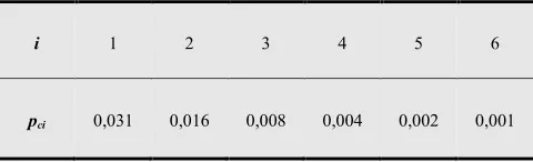
Table 1. The probability of collisions during the first attempt of data frame transmitting
і 1 2 3 4 5 6
рсі 0,031 0,016 0,008 0,004 0,002 0,001
From the values in Table 1 implies that if only two sta-tions are present in the network the probability of collisions during each subsequent attempt is not constant and de-creases by half.
Consider now the network, which contain only three ac-tive stations. We will consider only the collisions that occur between two stations, because the probability of collisions between the three stations is very small (more than an order of magnitude less). We consider the probability of collisions for the selected station, which due to previous collisions will make (m +1) attempts in order to convey data frame.
During the first attempt the collision may be with second station or with third station of network with the same probabilities equal to 1/CW1. The probability that the
se-lected station will avoid conflict with the second station is equal to (1–1/CW1), then the probability of collision with a
third station will be (1–1/CW1)⋅(1/CW1). Under these
con-ditions the full probability of collision for selected station in the first attempt will be equal to
) (
1 1
1 1
1 1 1 1
CW CW
CW
pc = + ⋅ − . (2)
On the second attempt in the system will be two stations that took part in the collision during the first attempt and use some random number to load their backoff counters from the range defined by contention window CW2. The third station
that has not experienced conflict during the first attempt will use the number from range defined by CW1. So, the total
probability of collision at second attempt for chosen station will be equal to
) (
1 2
1 2
1 1 1 1
CW CW
CW
pc = + ⋅ − . (3)
If the third attempt (i = 3) take place, selected station will use a contention window CW3 = [2і-1⋅(CWmin +1) – 1], the
other two stations – depending from their history will use the contention windows which defined by CW1 for one of them
and CW2 for other or CW1 and CW3 respectively. Under these
conditions the total collision probability may become one of the following:
) (
1 2
1 3
1 1 1 1
CW CW
CW p(I)
c = + ⋅ − ,
) (
1 3
1 3
1 1 1 1
CW CW
CW p(II)
c = + ⋅ − . (4)
Based on the result for the probability of collisions on the third attempt we can conclude that during the m-th attempt probability of collision will be determined by one of the ratios:
) (
1 2
1
1 1 1 1
CW CW
CW
p(I)cm= + ⋅ − ,
) (
1 3
1
1 1 1 1
CW CW
CW
pcm(II)= + ⋅ − , …,
) (
) (
1 1
1
1 1 1 1
CW CW
CW p
m )
M (
m
c + = + ⋅ − . (5)
Superscript notation of collision probability characterizes one of the possible values that can take the probability of collisions during the i-th attempt. Numerically M = m. Re-sults of calculations for the probability of collisions for one station in a network with three active stations are in Table 2.
Table 2. The probability of collisions on the network with three active stations
і 1 2 3 4 5 6
) (I ci
p 0,063 0,048 0,048 0,048 0,048 0,048
) (II ci
p 0,040 0,040 0,040 0,040
) (III ci
p 0,036 0,036 0,036
) (IV ci
p 0,034 0,034
) (V ci
p 0,033
Based on the analysis of the process of collisions, the ra-tios of (2) – (5), we can conclude that with the increase in the number of active stations in the network divergence values of collision probability during the various attempts to transmit a frame of information will decrease.
conclusions:
on networks which contain two or three active stations probability of collisions in the first attempt is considerably different from the probabilities of collisions which take place during next attempts. As a result, the application of universal analytical models for the analysis of such networks, which used a constant probability of collision, there are significant errors and discrepancies with the results of full-scale tests [4]. Consequently, to calculate the parameters and characteristics of such networks should apply some special mathematical models for two active stations and three active stations;
probability of collisions in wireless networks, where only two or three stations compete in order to get the channel, is small (рс << 1);
in order to develop a universal analytical model of the processes occurring in the channel of wireless network 802.11 with a number of stations N≥ 4 it possible to con-sider that the probability of collisions is constant for all attempts to transmit information frame and this probability is determined by the minimum value of contention windows and the number of stations in the network.
Based on the findings, it’s possible to propose the equa-tions for the probability of collisions during first attempt of data frame transfer in unplanned network with the number of active stations, more then four.
Let's find the probability of collisions as the total proba-bility, provided that collision involved each time only two stations. We shall find the probability of collisions that may happen during the first attempt. We must note that received so probability of conflict will be slightly inflated. The probability of collision between chosen station and one other station is p1c, with the second station (1– p1c)⋅p2c. Parameter
p2c is the probability of collision with second station only,
without taking into account other stations. Factor (1– p1c)
takes into account the probability that conflict with the first station will not happen. For the case of N stations in the network in general may be written
+ − − + − +
≈ c c( c) c( c)( c)
c p p p p p p
p 1 2 1 1 3 1 1 1 2
) (
... ) (
...+p(N−1)c 1−p1c ⋅ ⋅ 1−p(N−2)c
+ . (6)
If the collision probability with any other active station of the network will be the same and equal to pic = 1/CW1, using
(6) we shall obtain
+ + −
+ − +
≈ ( ) ( )2 ...
1 1
1 1
1
1 1 1 1 1 1 1
CW CW
CW CW
CW pc
1 1 2
1 1
1 1 1 1
1
1 − −
− − = −
+ N N
CW CW
CW ( ) ( ) (7)
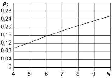
The collision probability in homogeneous networks (all stations have the same probability of access to the network), calculated by using of ratio (7), is shown in Fig. 1.
Figure 1. The dependence of collision probability for one wireless network station when it try to transmit the data frame for the case of CWmin = 31
4. The Wireless Channel Model of
Un-planned Network Of 802.11 Standard
We propose to consider a wireless channel model based on the use of virtual contention window. First of all it ne-cessary to find the value of virtual contention window VCW. We shall search it as the value of mathematical expectation for a binary exponential law of contention window CW increasing in case of collision, which is defined by basic specification of 802.11 standard
+ − +
−
= c pc pc
CW p
CW
VCW ( ) (1 )
2 2 1
2
1 1
= −
+ + −
+ m
c c m
c
c p p
CW p
p CW
) ( ...
)
( 1
2 2 1
2
4 1 2 1
∑
+= −
⋅ − ⋅ =
1
1 1 1
2 2
1 m
i i c
c p
p CW
) ( ) (
. (8)
A graphic dependence of the virtual contention window as a function of the number of active stations in the network shows in Fig. 2. Graph constructed using ratios (7) and (8).
Figure 2. Dependence of the virtual contention window VCW from the number of active stations on the network when used CWmin = 31
of about 1.22 time slots for each station.
Let's define now the probability of successful transmis-sion of a data frame each active station during a time of virtual contention window. We must define this probability as a total probability of a random process.
+ − + − + −
= 2
1 1
1 c c c c c
sc p p p p p
p ( ) ( ) ( )
1 1
1 1
1 1
1 +
+
− = − − − = −
+
+ m
c c
m c c m
c
c p
p p p p
p) ( )
(
... . (9)
During virtual contention window each station of network transmits an average of about one frame of data. More pre-cisely, this number is determined by the ratio (9). N stations transmit N frames.
Based on the concept of virtual contention window, it's possible to determine the number of collisions Nc, which
occurs on average when transmitting N frames of data. Based on the assumption that each collision involved only two stations, the number of conflict pairs will be equal to N/2.
We shall find the number Nc as the expected number of
collisions during a time of virtual contention window:
= + + + +
= m
c c
c c
c p
N p
N p N p N N
2 2
2 2
3 2
...
c m c c
p p N p
− − ⋅ ⋅
= +
1 1 2
1
. (10)
The obtained equations can be used to determine the throughput depending on the network settings. We can cal-culate throughput as the ratio between the average size of payload transmitted by all stations of network to time dura-tion of a virtual contendura-tion windows:
VCW
T PL E N
S ⋅ [ 1]
= , (11)
where - E[PL1] averaged payload of one data frame.
If the frame size will be constant the overall payload which transmitted during one virtual contention window will equal to N⋅PL1. The average duration of virtual contention
window will be
idle c c PL
VCW N T N T T
T = ⋅ + ⋅ + . (12)
To determine the values of time intervals TPL and Tc
we can use well-known relations, in particular, given in [2, 3]. Nc must be defined from (10). The average duration of
empty time interval Tidle that arise during the
implemen-tation of virtual contention window will be equal to
] ) (
[ m c
c
idle σ VCW N p N
T = ⋅ ⋅ ⋅ − +1 −
1 . (13)
By using (11) it possible to define the maximum meaning of throughput as a dependence of packet payload. The ex-pression (13) gives ability to get an accurate meaning of
idle
T duration.
The throughput, per one active station of the network will be therefore determined by the ratio
VCW
T PL E
S [ 1]
1= . (14)
Fig. 3 shows graphs of one station throughput as a func-tion of number of active stafunc-tions on the network. Charts are built using the ratio (14) for a network that operates accor-dingly to 802.11a standard at the speed of signal flow of 24 Mbit/s.
Figure 3. Dependence of one station throughput (S1) from the number (N)
of active stations on the network
5. Estimation of Quality of Service
Pa-rameters in Wireless Network
The ratios for some probabilities we got before give us ability to define some parameters of wireless network QoS. By using of some general expressions we can directly define such parameters as time delay of data packet transmission, the probability of data packet losing, jitter.
Time delay of data packet transmission over the wireless channel in accordance with the concept of virtual contention window will be equal to the duration of this virtual window,
VCW
T
=
τ . (15)
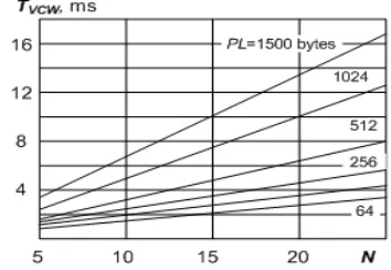
The average delay time of the data frame transmitting as a function of payload size for 802.11a network in the case of signal transmitting velocity of 24 Mbit /s by using of (12) shown on Fig. 4 - 5.
Figure 5. The transmission time delay as a function of size of payload in the data frame
The value of the probability of packet loss can be deter-mined directly from the ratio for the probability of suc-cessful transmission (9)
1
+
= m c rs
p
P( ) . (16)
Values of packet loss probability on a network with N stations calculated by using (16) is shown in Table 3.
Table 3.
N 5 10 15 20 25
P(rs) 2,9E-06 2,4E-04 2,1E-03 8,6E-03 2,3E-02
To determine the jitter σ(τ) make use of dispersion rela-tions for the delay of data frame
∑
−=
) (
) ( )
(
) (
b N
i i b
N
D 1 2
τ τ
τ , (17)
where N(b) – the total number of transmitted data frames and τі – transmission delay of a single data frame.
Based on the concept of virtual contention window, in order to define time dispersion we shall take into account the average value of transmission delay during each of the pos-sible attempts. In this case, expression (17) takes an other form, namely
∑
+=
− ⋅ =
1
1
2
1 m
j
j j
b N
N
D( ) ( * )
)
( τ τ
τ , (18)
where Nj and *
j
τ – the number of data frames and av-erage transmission delay during the j-th attempt respective-ly.
, )
( 1 1
1 1
2 2
1 −
− − ⋅ − ⋅ + ⋅ + ⋅ ⋅
⋅
= i
c i
i c PL c i
c *
j p
CW σ
p N T p p
N τ
)
( c
i c
j N p p
N = ⋅ −1⋅1− . (19)
Jitter expression we shall find by using of general formula and taking into account (18) and (19)
) (
) ( ) ( )
(τ τ τ τ
D
-σ = max min =2 , (20)
where τ( ) τ (τ),τ( ) τ (τ)
D
D min
max = + = − .
Graphs of σ(τ)=f(PL)
and σ(τ)= f(N) dependences for 802.11a network with signal stream at 24 Mbit/s, in which all the stations use CWmin = 31, calculated respectively with
(20) is shown in Fig. 6-7.
Figure 6. Uneven of transmission delay of the data frame (jitter) on a network with different number of active stations (N)
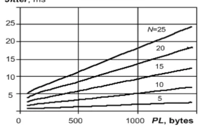
Due to graphs in Fig. 6, 7 we can conclude that the proc-ess of data frames transmitting over a wirelproc-ess network radio channel is characterized by considerable irregularity in time. This inequality essentially depends on the number of sta-tions in the network and the volume of payload in the data frame. Thus, for networks with N = 5, if the payload of a frame transmitted by the protocol UDP, is 64 bytes, jitter is 670 microseconds, and for the frame payload of 1024 bytes – 1742 microseconds.
Figure 7. Jitter as a dependence of payload in the data frame
For a network with N = 25 jitter is equal to 5521 and 17116 microseconds when the loads are 64 bytes and 1024 bytes respectively.
6. Conclusions
The proposed mathematical model of the wireless channel makes quantitative estimation of network operating pa-rameters and quality of service characteristics. If it known the number of active stations in the network, the minimum value of the contention window, size of data frame, the maximum value of the contention window and permissible number of retries to transfer data frame in the event of col-lisions we can get all probable parameters of wireless net-work channel.
The model obtained for a saturated mode of unplanned 802.11 network may be applied to network with moderate payload by specification of collisions probability.
References
[1] IEEE Std 802.11, 2007 Edition, Wireless LAN Medium Access Control (MAC) and Physical Layer (PHY) specifi-cation. – 3 Park Avenue, New York, NY 10016-5997, USA, June 2007. – 1232 p.
[2] Giuseppe Bianchi, Performance Analysis of the IEEE 802.11 Distributed Coordination Function/ Giuseppe Bianchi // IEEE Journal on Selected Areas in Communications. – 2000. – vol. 18 – №. 3. – p. 1055 – 1067.
[3] В.М.Вишневский. Широкополосные беспроводные сети передачи информации/ В.М.Вишневский, А.И.Ляхов, С.Л.Портной, И.В.Шахнович. – Москва: Техносфера, 2005, – 592с.
[4] Emerging Technologies in Wireless LANs. Theory, Design, and Deployment/ Edited by BENNY BING. – Georgia In-stitute of Technology, Cambridge University Press 2008. – 897p.
[5] V. M. Vishnevsky. 802.11 LANs: Saturation Throughput in the Presence of Noise/ V. M. Vishnevsky, A. I. Lyakhov // in Proc. IFIP Networking’02. – Italy, Pisa. – 2002.
[6] Z. Hadzi-Velkov and B. Spasenovski, “Saturation Through-put – Delay Analysis of IEEE 802.11 DCF in Fading Chan-nels,” in Proc. IEEE ICC’03, Anchorage, Alaska. – 2003, vol. 1. – pp. 121-126.
[7] Javier del Prado. Link Adaptation Strategy for IEEE 802.11 WLAN via Received Signal Strength Measurement / Javier del Prado, Sunghyun Choi // In Proc. IEEE ICC’03. – USA, Alaska, Anchorage. – 2003
[8] Daji Qiao. Goodput Analysis and Link Adaptation for IEEE 802.11a Wireless LANs / Daji Qiao, Sunghyun Choi,Kang G. Shin // IEEE Trans. on Mobile Computing (TMC). – 2002. - vol. 1, № 4. – pp. 278-292
[9] Jean-Lien C. Wu. An Adaptive Multirate IEEE 802.11 Wireless LAN / Jean-Lien C. Wu, Hunh-Huan Liu, Yi-Jen Lung // in Proc. 15th International Conference on Informa-tion Networking – 2001. – pp. 411-418.