DISCRETE WAVELET TRANSFORM
AND S-TRANSFORM BASED TIME
SERIES DATA MINING USING
MULTILAYER PERCEPTRON NEURAL
NETWORK
LALIT KUMAR BEHERA1
Department of Computer Science and Engineering
Asst. prof.,Gandhi Institute for Technological Advancement,BBSR,India
MAYA NAYAK2
Department of Information Technology Professor,Orissa Engineering College,BBSR,India
SAREETA MOHANTY3
Department of Information Technology Sr. Lecturer,Orissa Engineering College,BBSR,India
Abstract:
This paper presents discrete wavelet transform and the S-transform based neural classifier scheme used for time series data mining of power quality events occurring due to power signal disturbances. The DWT and the S – transform are used for feature extraction and then the extracted features are classified with neural classifiers such as multilayered perceptron network (MLP) for pattern classification, data mining and subsequent knowledge discovery.
Keywords: Time series database; DWT; S-transform ; Neural network ; Feature extraction ; Classification. 1 . Introduction:
As the development of power industry and the application of power electronic equipments in power system is gaining momentum , the problems of power quality, like voltage sag, voltage swell, voltage interruption, harmonics , voltage notch, and different combination like (sag + harmonics) etc., have also aroused great attention. The difference of time domain signal among power quality problems is not obvious, so, feature extraction and classification for problems of power quality has important significance.
The main methods used in feature extraction for problem of power quality are wavelet transform, windowed Fourier transform[1], d-q transform[2], kalman filtering [4]etc., and the main method for automatic classification is neural network. [6] . The calculation of Fourier transform is simple and easy to realize, but, Fourier transform is not suitable for the analysis of power quality disturbances because of its poor localizing ability for time and frequency. Wavelet transform is time-scale analysis, and the scale according to wavelet function is not corresponding to the frequency, and the transformation process is complex, the result is lacking directness and easy to be affected by noise.
the visually distinguishable patterns to feature vectors that can be used by classifiers such as neural networks to automatically classify the disturbances.
2 . Wavelet Transform basics :
The Continuous Wavelet Transform (CWT) associated with the mother wavelet
ψ
( )
t
is defined as:
W a b
( , )
y t
( )
ψ
*a b,( )
t dt
∞ −∞
=
(2.1)where
y t
( )
is any square integrable function, a is the scaling parameter, b is the translation parameter and ,( )
a b
t
ψ
is the dilation and translation of the mother wavelet defined as:a b,
( )
t
1
t
b
a
a
ψ
≡
ψ
−
(2.2)This CWT provides a redundant representation of the signal in the sense that the entire support of
W a b
( , )
need not be used to recovery t
( )
. By only evaluating the CWT at dyadic intervals, the signal can be represented compactly as:
( )
( )2
2(
2
)
j j j
k j
y t
d k
ψ
t
k
∞ ∞ =−∞ =−∞
=
−
(2.3)where
d k
j( )
is called the discrete wavelet transform (DWT) ofy t
( )
.Associated with the wavelet is a scaling functionϕ
( )
t
. The scaling function along with the wavelet creates a multiresolution analysis (MRA) of the signal. The scaling function of one level can be represented as a sum of a scaling function of the next finer level.( )
( ) 2 (2
)
n
t
h n
t
n
ϕ
∞ϕ
=−∞
=
−
(2 .4)The wavelet is also related to the scaling function by
( )
1( ) 2 (2
)
n
t
h n
t
n
ψ
∞ϕ
=−∞
=
−
(2.5)We can make use of the scaling function to represent the signal as:
( )
( )2
2(2
)
( )2
2(2
)
jo j
jo j
jo j
k k j jo
y t
c k
ϕ
t k
d k
ψ
t k
∞ ∞ ∞
=−∞ =−∞ =
=
− +
−
(2.6)where
jo
represents the coarsest scale spanned by the scaling function. The scaling and wavelet coefficients of the signaly t
( )
can be evaluated by using a filter bank of quadrature mirror filters (QMF).j
( )
j 1( ) (
2 )
m
c k
c
m h m
k
∞ + =−∞
=
−
(2.7)j
( )
j 1( ) (
12 )
m
d k
c
m h m
k
∞ + =−∞
=
−
(2.8) Eq (2.7) and (2.8) show that the coefficients at a coarser level can be attained by passing the coefficients at the finer level to their respective filters followed by a decimation of two. This will result in the number of samples in the coarser level to be approximately half of the number of samples at the finer level.
3 . S-Transform basics:
The S-Transform of a time series
y t
( )
is defined as:
(
)
2( , )
( )
,
i ftS
τ
f
y t g t
τ
f e
π∞
− −∞
=
−
(3.1)2 2 2
( , )
2
tf
g
τ
f
e
σπ
−
=
(3.2)with the spread parameter inversely proportional to the frequency
1
f
σ
=
(3.3)The final expression becomes 2 2 ( ) 2 2
( , )
( )
2
t f i ftf
S
f
y t
e
e
dt
τ π
τ
π
∞ − − − −∞=
(3.4)where f is the frequency, t and τ, are both time.
The S-Transform of the continuous time function
y t
( )
can also be defined as a CWT with a specific mother waveletW
(
τ
,
d
)
multiplied by a phase factor.
2
( , )
i f( , )
S
τ
f
=
e
π τW
τ
d
(3.5) Where the mother wavelet is defined as
W
( )
τ
,
d
y t w t
( ) (
τ
, )
d dt
∞ −∞
=
−
(3.6)and ft i f t
e
e
f
f
t
ππ
ψ
2 22 2
2
)
,
(
=
− − (3.7)where the dilation factor is the inverse of the frequency f.
The phase factor in Eq (3.5) is in fact a phase correction of the definition of the Wavelet Transform. It eliminates the concept of “wavelet analysis” by separating the mother wavelet into two parts, the slowly varying envelope (the Gaussian function) that localizes in time, and the oscillatory exponential kernel that selects the frequency being localized. It is the time localizing Gaussian that is translated while the oscillatory exponential kernel remains stationary. By not translating the oscillatory exponential kernel, The S-Transform localizes the real and imaginary components of the spectrum independently, localizing the phase spectrum as well as the amplitude spectrum. This is referred to as absolutely referenced phase information.
The choice of windowing function is not limited to the Gaussian function. Other windowing function was tried with success. The inverse S-Transform is given by
2
( )
( , )
i fty t
S
τ
f d
τ
e
πdf
∞ ∞ −∞ −∞
=
(3.8)and since
S
( , )
τ
f
is complex, it can be written as( , )
( , )
( , )
i fS
τ
f
=
A
τ
f e
θ τ (3.9)Where
A
( , )
τ
f
is the amplitude of the S-spectrum andθ τ
( )
,
f
is the phase of the S-spectrum.The phase spectrum is an improvement on the wavelet transform [11] in that the average of all the local spectra does indeed give the same result as the Fourier Transform. Eq- (3.4) is derived on the assumption that the spread of the Gaussian modulation function is proportional to the inverse of frequency. To increase the frequency resolution, the spread of the Gaussian window σis written as
f
α
σ
=
(3.10)and the generalized S-Transform is obtained as
2 2 2 ( ) 2 2
( , )
( )
2
t f i ftf
S
f
y t
e
e
dt
τ π α
τ
α π
− ∞ − − −∞=
(3.11)In Eq (3.10) α controls the frequency resolution. If α is above 1, the frequency resolution would increase. Likewise if α is below 1, the time resolution improves.
S y
{
noisy( )
t
}
=
S y t
{ } { }
( )
+
S
η
( )
t
(3.12)The amplitude and phase spectrum of S-transform are given by
))
)
,
(
Re(
/
)
)
,
(
(Im(
)
,
(
))
,
(
(
j
n
S
j
n
S
ang
j
n
j
n
S
abs
A
=
=
φ
(3.13)The discrete version of the S-Transform of a signal is obtained as
[
]
Nmj i N m
e
n
m
W
n
m
Y
n
j
S
π 2 1 0]
,
[
]
,
[
− =+
=
(3.14)where Y[m + n] is obtained by shifting the discrete Fourier Transform (DFT) of y(k) by n, Y[m] being given
[ ]
N mk j N ke
k
y
N
m
Y
π 2 1 01
]
[
− − =
=
(3.15)
2 2
-2πmβ
n
W[m+ n] = e
(3.16)Where j, m and n = 0, 1, ….., N-1 . Another version of the discrete S-Transform used for computation
[
]
N -1
2πnm 2 2πnk
-j i * N N N k=-2
S[m,n] = e
x m+ k w (k,n)e
for m = 1, 2, …, M and n = 0, 1, 2, …N/2 (3.17)where M is the number of data points of the signal y[m], N is the width of the window, the signal vector y[m] is padded at the beginning or at the end with 0.
The output of the S-Transform is a matrix whose rows pertain to time and whose columns pertain to frequency. This matrix called the S-Matrix contains all the values of the complex valued S-Transform output. The computation of the S-Transform is efficiently implemented using the convolution theorem and FFT. The following steps are used for the computation of S-Transform:
(1) Compute the DFT of the signal y(k) using FFT software routine and shift spectrum Y[m] to
Y[m+n].
(2) Compute the Gaussian window function
exp(-2
π β
2 2m /n )
2 2 for the required frequency n. (3) Compute the inverse Fourier Transform of the product of DFT and Gaussian window functionto give the ST matrix. 4 . Feature Selection :
4.1. Based on Wavelet Transform:
There are many different wavelet based methods reported in the literature for feature extraction. They involve performing some kind of transformation on the DWT coefficients, comparing between the DWT coefficients of the disturbance signal with the DWT coefficients of a pure signal, compressed DWT coefficients, direct use of the DWT. comparing the performance of and the hybrid FFT-DWT methods for pattern classification of electrical network disturbances along with the new approach based on statistical feature selection by S-transform. Each disturbance will give a different signature that can be used for classification purposes.
4.2. Feature Selection Based on S-Transform:
The output from the S-Transform is an N by M matrix called the S-matrix whose rows pertain to frequency and whose columns pertain to time. Each element of the S-matrix is complex valued. The S-matrix can be represented in a time-frequency plane similar to that of the wavelet transform. Here
α
is normally set to 0.4 for best overall performance of the S-Transform, where the contours exhibit the least edge effects and for computing the highest frequency component of an oscillatory transient waveformα
is set equal to 1 or 3 as required.Feature extraction[12] is done by applying standard statistical techniques to the contours of the S-matrix as well as directly on the S-S-matrix. These features have been found to be useful for detection, classification or quantification of relevant parameters of the signals. The power network signal is normalized with respect to a base value, which is the normal value without any disturbance. The resolution factor α was set to 0.4 for better time resolution. Four features were extracted from the S-transform output. Few are:
F1 = max (A)+min (A)-max (B).where A is the amplitude versus time graph from the S-matrix under
deviation (
σ
) of contour No.1 having the largest frequency ,F
3= Energy ,F
4=
Total harmonic distortion ofthe signal i.e.
1 2
2
V
V
THD
N
n n
=
=
where N is the number of points in the FFT,V
nthe value of the nthharmonic component of the FFT. ,
F
5=
Maximum Frequency of the signal ,F
6=
Mean of the lowestcontour above twice the normalized fundamental frequency,
F
7=
Skewness Cr3 1
3
(
)
(
1)
N
i i
y
y
N
σ
− =
−
=
−
,
F
8=
max(
Cr
) min(
−
Cr
)
,F
9=
Standard deviation of Cr. where Cr is the amplitude versus time graph of the S-matrix for frequencies above twice the normalized fundamental frequency magnitude versus time,F
10=Average power for frequencies above 2.5 times the fundamental frequency . These features are found to be well suited to distinguish the twelve classes of power quality disturbances like Normal, Sag, Swell, Momentary Interruption (MI), Harmonics, Sag with Harmonic, Swell with Harmonic, Flicker, Notch + Harmonics, Spike + Harmonics, Transient (low frequency),Transient (high frequency).5 . Wavelet based Neural Classification Schemes :
Three different wavelet based techniques are outlined here for nonstationary time series that occur in power networks due to various stochastic disturbances. They are denoted as Methods 1 and 2. Each of these described methods yields classification accuracy of the temporal signal patterns occurring due to power network disturbances (also known as power quality events).Method-1 (WT-1) was implemented using the thirteen level coiflet 5-wavelet decomposition. The de-noising step in Method-2(WT-2) was omitted to test its effectiveness in noise
The pattern classification results are then summarized for the above four techniques, namely DWT based energy calculations; DWT based statistical parameters, the hybrid DWT and DFT based approach. When a large data set is encountered the computational overhead for the wavelet and other signal processing methods increases and in such a case the entire data is partitioned into several sections and classification and finding similarity is attempted for each partitioned section. Processing methods increases and in such a case the entire data is partitioned into several sections and classification and finding similarity is attempted for each partitioned section. In the next section different DWT based methods are described for feature extraction and automatic pattern classification.
5 . 1 . Method-1 (WT-1):
If the scaling function and wavelets form an orthonormal basis, then Parseval’s theorem relates the energy of the distortion in the signal to the energy of the expansion components and their wavelet coefficient. Parseval’s theorem is given as:
2
2 2
( )
( )
( )
signal j
k j jo k
E
y t
dt
c k
d k
∞ ∞ ∞ =−∞ = =−∞
=
=
+
(5.1.1)The energy of the signal at different resolution levels can be computed as:
E
signalc
od,
d
od,...,
d
(J−1)d
=
(5.1.2)od od
( )
2k
c
c
k
∞ =−∞
=
(5.1.3)and
2
( )
jd jd
k
d
d
k
∞ =−∞
=
(5.1.4)where || || is the
L R
2( )
norm and J represents the total number of resolution levels,c
od( )
k
is the approximation DWT coefficient andd
jd( )
k
is the detail DWT coefficients for the disturbance signal at level j
x
0= Δ =
E
E
signal−
E
pure (5.1.5)5 . 2 . Method-1 (WT-2):
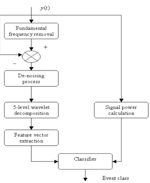
Statistical calculations are done on the DWT coefficients of the fifth level detail coefficients together with signal power to yield the following features:
(1) The mean value of
d k
5( )
(2) The standard deviation ofd k
5( )
(3) The maximum modulus coefficient of
d k
5( )
(4) Signal power,P k
( )
The four-dimension feature vector
x
0is given a
x
0=
mean d k
(
5( ) ,
)
std d k
(
5( ) , max
)
d k
5( ) , ( )
P k
(5.2.1)
Fig .1 . Block diagram of classification algorithm
6 . S-Transform based Neural Classifier:
For steady state short-time disturbance signal patterns like voltage dip, voltage swell, and voltage interruptions time series, the value of F1 varies from 0.05 to 0.90, and from 1.15 to 1.8. However, for single and multiple
notched time series this value lies between 0.85 and 0.98. For normal, oscillatory transients, impulsive transients, the value of F1 lies between 1.0 and 1.08. The standard deviation feature F2 is less than 0.05 for the
The energy feature F3 is less than 0.03 for the transients and for all other signals it varies between 0.05 and 0.1.
Other features like mean, skewness, and factors can provide distinction between patterns. In a practical situation the time series data collected from the power network could run into several gigabytes and in such a case the data is partitioned into several sections and feature extraction is attempted for each partitioned section. Also in a large data set similar disturbance pattern exists and this can be easily identified from these features with the help of trained neural networks.
Table-1. Classification result with MLP
MLP
Pure 30dB
Method WT-1 WT-2 ST WT-1 WT-2 ST
Oscillatory
transient 95% 95% 90% 30% 90% 95%
Impulsive transient 100% 70% 95% 100% 65% 85%
Multiple notch 100% 85% 100% 90% 85% 100%
Voltage swell 100% 100% 100% 55% 95% 100%
Voltage sag 90% 80% 80% 60% 85% 96%
Interruption 100% 90% 100% 100% 95% 100%
Harmonics 100% 85% 90% 15% 80% 85%
Swell +
Harmonics 100% 95% 100% 60% 95% 100%
Sag +harmonics 100% 80% 100% 25% 80% 100%
Average 98.33% 86.67% 95% 59.44% 85.56% 83.4%
Three Multilayer Perceptron was trained using the various extracted features and are used as classifiers. The network is trained in batch mode with a total of 300 training vectors representing the ten different classes. The feed forward network is trained for 1000, 1500, and 2000 epochs with the goal set at 1% mean square error. A test vector of 150 signals is used for testing the neural network. The network is also tested with signals added with 30dB of white Gaussian noise. Different spread values were tried to obtain the best results. The classification results are shown in Tables 1.
9. Conclusion
10. References:
[1] Heydt G T, Fjeld P S, Liu C C, et al, "Applications of the windowedFFT to electric power quality assessment, " IEEE Transaction on Power Delivery, vol.14, pp. 1411-1416, 1999.
[2] Xu, Yonghai. Xiao, Xiangning. Song, Y.H, "Automatic classificationand analysis of the characteristic parameters for power qualitydisturbances, " IEEE Power Engineering Society General Meeting,vol.1, pp. 496-503, 2004.
[3] Stockwell R G, Mansinha L, Lowe R P, "Localization of the complexspectrum: The S-transform, " IEEE Transactions on Signal Processing,vol. 17, pp. 998-1001, 1996.
[4] P. K. Dash, M. V. Chilukuri, "Hybrid S-Transform and Kalman Filtering Approach for Detection and Measurement of Short Duration. Disturbances in Power Networks, "IEEE Transactions on Instrumentation and Measurement, vol. 53, April 2004.
[5] Dash, P.K. Chilukuri, M.V. Panigrahi, B.K, "Power quality analysis and classification using a generalized phase corrected wavelet transform, "IEE Conference Publication, No. 487, pp. 610-615, 2002.
[6] Damarla, G.P. Chandrasekaran, A. Sundaram, Ashok, "Classification of power system disturbances through fuzzy neural network, "Canadian Conference on Electrical and Computer Engineering, vol. 1, pp. 68-71,1994
[7] I.W.C.Lee, and P.K.Dash, “ S-Transform based Intelligent system for classification of power quality disturbance signals” IEEE Transactions on Industrial Electronics, vol.50, no.4, August 2003, pp.800-806.
[8] W.C. Lee and P.K. Dash, “An S-transform based Neural Pattern Classifier for Non-Stationary Signals,” Proc. 6th International Conference on Signal Processing, 2002.
[9] P.K. Dash, B.K. Panigrahi, and G. Panda, “Power Quality Analysis using S-transform”, to appear in IEEE Trans. on Power Delivery, vol.8, no.2, April 2003, pp.406-412.
[10] Varanini, M., Paolis, G.D., Emdin, M., Macerata, A., Pola, S., Cipriani, M., & Marchesi, C, “A multiresolution transform for the analysis of cardiovascular time series” Computers in Cardiology, vol.25, 1998, pp.137-140.
[11] D. Borras et al, “Wavelet and neural structure: A new tool for diagnostic of power system disturbances,” IEEE Trans. on Industry Applications, vol.37, no.1, pp.184-190, 2001.