1269
Volume 63 140 Number 4, 2015
http://dx.doi.org/10.11118/actaun201563041269
A PREDICTIVE LIKELIHOOD APPROACH
TO BAYESIAN AVERAGING
Tomáš Jeřábek
1, Radka Šperková
21 Faculty of Economic Studies, University of Finance and Administration, Estonská 500, 101 00 Praha 10, Czech Republic
2 Department of Economy and Management, College of Business and Hotel Management, Bosonožská 9, 625 00 Brno, Czech Republic
Abstract
JEŘÁBEK TOMÁŠ, ŠPERKOVÁ RADKA. 2015. A Predictive Likelihood Approach to Bayesian Averaging. Acta Universitatis Agriculturae et Silviculturae Mendelianae Brunensis, 63(4): 1269–1276.
Multivariate time series forecasting is applied in a wide range of economic activities related to regional competitiveness and is the basis of almost all macroeconomic analysis. In this paper we combine multivariate density forecasts of GDP growth, infl ation and real interest rates from four various models, two type of Bayesian vector autoregression (BVAR) models, a New Keynesian dynamic stochastic general equilibrium (DSGE) model of small open economy and DSGE-VAR model. The performance of models is identifi ed using historical dates including domestic economy and foreign economy, which is represented by countries of the Eurozone. Because forecast accuracy of observed models are diff erent, the weighting scheme based on the predictive likelihood, the trace of past MSE matrix, model ranks are used to combine the models. The equal-weight scheme is used as a simple combination scheme. The results show that optimally combined densities are comparable to the best individual models.
Keywords: predictive likelihood, density forecasts, Bayesian averaging, Bayesian VAR model, GDP growth, infl ation, real interest rates
INTRODUCTION
A combining forecasts from diff erent models to increase their forecast accuracy belongs to the popular macroeconomic research techniques and the fi rst studies in this area have been focused on combining point forecasts; see Timmermann (2006). However, the point forecast evaluation does not take into account a model uncertainty. The solution is the knowledge of the probability distribution of the individual forecasts and therefore density forecasts can be used instead of the point forecasts. As reported in Hall and Mitchell (2007) combining density forecasts provide more accurate description of the true degree of the uncertainty. An empirical question depends on the method used to choose weights for individual models when the combined densities are constructed. A natural way to choose weights in a Bayesian context is to use posterior probability weights based on the marginal likelihood for each model. Unfortunately, there are two problems for the posterior probability weights. The fi rst, the weights are infl uenced by the number
solution; see Eklund and Karlsson (2005). Therefore, the above authors estimate of the predictive likelihood by using the normal kernel density estimation from the predictive draws. However, Adolfson et al. (2007) show that this approach is not practical unless the dimension of density forecast is small and they suggest using a normal approximation of the predictive likelihood based on the mean and the covariance of the marginal predictive distribution. Warne et al. (2013) show that predictive likelihood can be computed via missing observations techniques.
This paper proposes to combine trivariate density forecasts from two BVAR, models, a DSGE and a DSGE-VAR model. Several methods to combine forecasts from the set model are considered – predictive likelihood based weights following Adolfson et al. (2007) approach as well as Warne
et al. (2013) approach, the relative performance
weights based on the trace of past MSE matrix, and the weights based on model ranks. The equal-weight scheme is used as a simple combination scheme.
MODELS AND DATA
I consider four models of the Czech Republic economy. Two variants of Bayesian VAR model with 4 lags for endogenous and 4 lags for exogenous variables. The Minnesota prior is used. This prior is based on an approximation which leads to
shrinking the parameters towards zero by assuming that the observed variables of model follow independent random walks; see Doan et al. (1984) and Koop and Korobilis (2010). The individual variants of BVAR model diff er from one another by setting of the overall tightness parameter which controls the prior standard deviations of all the lag coeffi cients of the endogenous variables. I set value for BVAR1 and value 0.2 for BVAR2. The values for another hyperparameters were chosen according to Jeřábek et al. (2013). I generate 10 000 draws from posterior distributions using Gibbs Sampler with the fi rst 500 draws used as burn-in sample which is removed.
The DSGE model is constructed as a small open economy model and it is borrowed from Seneca (2010). The model parameters are chosen through a combination of calibration and formal estimation, according to Seneca (2010) and Musil (2009). The posteriors of the estimated parameters are simulated using 500 000 draws from the Random-Walk Metropolis-Hastings algorithm where the fi rst 100 000 are removed.
Furthermore, the DSGE model is used to generate a prior distribution for the coeffi cients of the VAR model, i.e. DSGE-VAR model. As referred by Del Negro and Schorfheide (2004), this prior concentrates most of its probability mass near the restrictions that the DSGE model imposes on the VAR representation and pulls
1: Selection of the optimal
Source: authors
I: Model overview1
Type Eq. Par. Est. Par. Observed variables
BVAR with 4 lags 11 59 59 Endogenous: GDP, consumption, investment, government spending, import, export, hours worked, real exchange rate, CPI infl ation, wage infl ation, interest rate.
Exogenous: CPI infl ation, GDP, interest rate.
DSGE 62 68 42
DSGE-VAR with 4 lags 11 59 59
Source: authors
the likelihood estimate of the VAR parameters toward the DSGE model restrictions. The DSGEVAR model is indexed by -value which measures the deviation of the DSGE-VAR from the VAR approximation of the DSGE model; see Del Negro and Schorfheide (2012). For the optimal -value choice, I use of the maximize marginal likelihood for the estimations of the DSGE-VAR with lags 1 up to 4 over [0, ∞]. As seen from Fig. 1, the optimal model choice results in 1 lags and = 2.8.
METHODS
For the formulation of conclusions and recom-mendations from the methodological point of view use the following methods.
Model Averaging
A combination density forecast pc is constructed
as a weighted linear combination of the model forecasts, i.e.
1
+ 1, , , , , , +
=1
,…, , ,…, )
( ) (
M
c M m
t t t
t h h t M h t m h t t h
m
p z p z ,
(1) where the vector consists three variables GDP growth, CPI infl ation and interest rate, and p(zt+h|tm)
is trivariate density forecast for horizon h = 1, …, H of model m = 1, …, M at time t, t
m is the information
set of model including model parameters, variables and equations. Four diff erent weighting schemes are used. The weights m,h,t are based on the predictive
likelihood, the trace of mean square errors (MSE) matrix of past forecasts, the relative past forecasting accuracy by assigned ranks from 1 to M according to accuracy measured by the trace of the MSE and the mean forecasts – equal weights.
Predictive Likelihood Weights
The approach based on the predictive likelihood requires to split data into a training sample for estimate the models and hold-out sample used to evaluate forecasting performance of models. As in Gerard and Nimark (2008), the predictive likelihoods are calculated over a recursive scheme where the training sample Yt = (y1, …, yt)’ relevant to
period t is extended by one observe at each recursive step, where vector y consists all observed variables. Let Zt,h = (zt+h, …, zT)’ be hold out sample at horizon h. For the predictive likelihood p(Zt,h|Yt, m) for model
m at horizon h holds p(Zt,h|Yt, m) = ∏t
T = − 1 h p(z
t+h|Yt,m). (2)
The predictive likelihood weights are given by
, , , =1 ( , ) ( , )PL t.h t
m h t M
t t h i
p Z Y m
p Z Y i
. (3)
I use two approaches to evaluate of the marginal predictive likelihood (MPL) p(zt+h|Yt, m). The fi rst method consists in MPL approximation by normal MPL which is based on the mean and the covariance of the marginal predictive distribution, see Adolfson
et al. (2007). Hence, to evaluation equation (2),
for each model m the normal distribution is used and I take an average across multiple draws from model m’s marginal predictive distribution. That is
+ 1 1( , ) S j( , )
t N t
t h t h
j
p z Y m p z Y m
S , (4)
where S = 500 and pN(zt+h|Yt, m) is normal MPL.
The second approach – as in Warne et al. (2013), I use an importance sampling (IS) estimator for calculate the marginal predictive likelihood in (2), see, e.g., Koop (2003). With j being draws from
the importance density q(j|m), an expression of
the IS estimator is
=1 ( , , ) ( , ) 1 ( , ) ( ) nt j j t
t h t
t h
j j
p z Y m p Y m
p z Y m
n q m , (5)
where n = 10000. I use the cross-entropy method for select the importance density; see Rubinsteinem (1997) and Chan and Eisenstat (2012).
MSE Based Weights
This approach is based on the trace of the h -step-ahead MSE matrix ∑M(h) of past forecasts. Weights
are built on the relative past forecasting accuracy by ranking the accuracy of the models. Thus, MSE based weights are computed by taking forecasts from previous periods and evaluate of the trace of MSE matrix for each model. For the h-step-ahead MSE matrix holds
M
( ) 1 +
h1T N
t T h h
N ϵ˜t+h|tϵ˜’t+h|t, (6)
where ϵ˜t+h|t = M −1/2ϵ
t+h|t, where ϵt+h|t stand for the error h
– step predictions made during the t and M is a positive defi nite matrix – I use M as an unit matrix. The weights are then calculated through the inverse relative MSE performance
, , , 1 , 1 1 m h t MSEm h t M
i
i h t
MSE
MSE
, (7)
where MSEm
h,t is the trace of ∑M(h) belong to model m
and for period t.
RANK Based Weights
Another approach to determinate relative performance weights is based on assigning ranks R
by evaluate the trace of MSE matrix. These weights are computed as
, , ,
1 ,
1
1
m h t R
m h t M
i i h t
R
R
. (8)
Equal Weights
This is the simplest weighting scheme and consists in putting equal weight on all model in the suite. Thus, in this case holds E
m W
,h,t=1/m for each forecast
horizon.
IMPLEMENTATION AND RESULTS
The data sample is given by the period 1999:Q1 until 2012:Q4 and a recursive out-of-sample forecasting scheme was used to evaluate of models and generate weights for each model. The sample from 1999:Q1 to 2006:Q4 was used as initial training sample to estimate of models and to construct density forecast up to twelve quarters ahead, from 2007:Q1 to 2009:Q4. Then, models were estimated for the extended training sample (by one observation), 1999:Q1–2007:Q1, and density forecasts were constructed over the next twelve quarters, i.e. from 2007:Q2 to 2010:Q1, and so on. The fi nal training sample was between 1999:Q1 and 2012:Q3, which allows forecast for period 2012:Q4.
Trivariate density forecasts on the right side of the equation (1) were constructed by taken of multiple draws from posterior parameter
distribution of each model and by iterative making of trivariate density realizations forward up to horizon h = 12 for each draw. Complete density forecasts have been built by repeating 2500 times at each forecast horizon; see Adolfson et al. (2007) or Christoff el (2010) for algorithm.
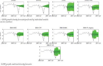
As an example, the univariate density forecasts for GDP growth that have been obtained using data up to 2008:Q2 for each model; see Fig. 1. The black curve shows observed data until forecast start. The diff erent shades show various confi dence bands, from 5% to 95%. The line in the middle of the bands shows the mean forecast for each model. I chose the period 2008:Q3, when U.S. bank Lehman Brothers failed and GDP growth turned negative, as start forecasts to compare the forecasting accuracy of models during crisis and recession. Fig. 2 shows that the BVAR models are not able to predict recession. GDP growth is predicted to stay almost constant by BVAR1 and BVAR2 as in 2008:Q2. Very similar results show DSGE and DSGE-VAR models. It may be seen that the BVAR models perform well in terms of density forecast accuracy against DSGE a DSGE-VAR giving higher degree of the forecast uncertainty. Thus, the non-structural models give less uncertainty than structural models and their forecasts do not perform well during the recession. Fig. 2 shows the combined density forecasts for GDP growth derived from the same period as the density forecasts for the individual models. It is seen that the weighting schemes prefer structural model at period of recession, which is in line with the results from the density forecasts of individual model on Fig. 3.
2: GDP growth density forecasts predicted by individual models Source: author
Fig. 4 shows the mean forecast paths from the univariate densities for individual BVAR1, BVAR2, DSGE and DSGE-VAR models together with the data for GDP growth. It is obvious that
the forecast paths of the BVAR models with Minnesota type prior are more or less constant for all observed periods. More accurate mean forecasts provide another two models. The forecast paths 4: GDP growth combined density forecasts
Source: authors
for the DSGE-VAR model and the DSGE model are similar to each other. The lowest mean forecast errors are given by DSGE model. This result is confi rmed by used forecast error statistics, see Fig. 6 (the fi rst line).
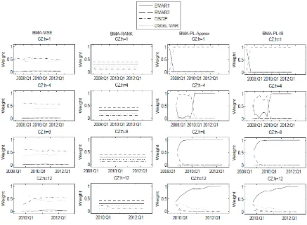
How the weights are evolved through the hold-out sample is shown in Fig. 5 for one, four, eight and twelve – step – ahead – forecasts. Five diff erent model weights are used – the weights based on the MSE matrix, model rank and two approaches to the predictive likelihood evaluation. The equal weights are used, as well. It may be seen that the weights based on the trace of the h-step-ahead MSE matrix prefer DSGE and DSGE-VAR model with very similar weights. BVAR model weights were assigned value equal to zero. This is consistent with the statement according to the Fig. 4 which shows that DSGE and DSGE-VAR models provide the most accurate point forecasts. Rank based weights assigned the highest rank to the BVAR2
model and the lowest weights to DSGE model over all observed forecast horizons. The rank weights are as well as MSE weight computed based on the trace of the h-step-ahead MSE matrix. The diff erences between MSE weight and rank weight are caused by more cautious approach to the rank based weight algorithm – none of the models can be exclude and extremely preferred. Both approaches to the predictive likelihood provide very similar results. The weights assigned by both the approximation approach and importance sampling approach are almost identical. The models with lower degree of the forecast uncertainty are preferred.
The combined point forecast of models m for horizon h are determined as mean of combined density forecast (1). The forecast comparison covers both the univariate measures based on RMSE and the multivariate MSE-based measures with log determinant and trace of the MSE matrix (6); see Warne et al. (2013). Figs. 6 and 7 show point forecasts
6: RMSE of models Source: authors
comparison of individual and combined forecasts where the bold line represents of combined forecasts. It may be seen that a model performing well in terms of density forecast accuracy does not necessarily make the most point forecasts accuracy. As indicated above, two type of the BVAR models used in the paper have higher density accurate against DSGE and DSGE-VAR models. But it is clear that the combined forecasts have in general an accuracy higher than forecasts from most single models.
From individual models, the results for observed variables are diff erent from each other. The RMSE statistic shows that the DSGE-VAR model provides the best result for the infl ation as well as GDP growth, as already mentioned. Conversely, this model fails for the real interest rate. We fi nd that the forecasting accuracy of the DSGE and the DSGEVAR model is very similar from both the univariate RMSE and the multivariate trace MSE view. When using the multivariate log determinant MSE statistic, the DSGE model outperforms DSGE-VAR model. The contradiction for forecast evaluation between two use multivariate statistics is described by Herbst and Schorfheide (2012).
There is no much diff erence between the accuracy of the combined models each other evaluated by the RMSE statistic except interest rate estimated by predictive likelihood weighting scheme for the longer horizons – from eight quarter ahead horizon forecasts. MSE statistic provides an overall view of forecasts. As reported by Timmerman (2006), the equal weighted mean forecast combinations are diffi cult to overcome in terms of accuracy. The trace of the MSE matrix, which is infl uenced by the least predictable variables, shows that the rank based weight yields more accurate forecasts against other models. But, an increase of the forecast accuracy is diffi cult to excuse by increasing of the computational eff ort equated to the equal weighting forecasts. Thus, weighting scheme that
give signifi cant weight to more models are preferred over weighting scheme that assign high weight to one or two models. The MSE log determinant statistic is infl uenced by both the most and the least predictable variables.
DISCUSSIONS
In this paper, we dealt with only little explored part of the economy forecast area, namely combining multivariate density forecasts. At the fi rst, we have compared the accuracy of mean trivariate density forecasts of two BVAR models, DSGE model and DSGE-VAR model. The mean forecasts were observed from both the univariate and multivariate view. Forecast accuracy of DSGE model is comparable to the forecasting accuracy VAR model. Especially, DSGE-VAR and DSGE models yield relatively precise GDP growth and infl ation, they overcome non-structural BVAR models. However, DSGE-VAR fails for interest rate forecasts, when DSGE model provide the higher forecast accuracy. Thus, forecast accuracy used models are diff erent. For overcoming this problem the combining forecasts from several models were used. We have employed fi ve diff erent weighting scheme based on the trace of the MSE matrix, the model rank, two approaches to the predictive likelihood compute and equal weight. The weighting schemes based on predictive likelihood assign almost zero weights to DSGE and DSGE-VAR model in the combined density forecast. This is due to high uncertainty of the model density forecast. There is not much of a diff erence between the accuracy of the other combination schemes. Weight forecasts increase the forecasting accuracy. The rank based weight and equal weigh model yield more accurate forecasts against other models. Results show that weighting scheme that give signifi cant weight to more models are preferred over weighting scheme that tend to consider one best model.
CONCLUSION
Acknowledgement
This work is supported by funding of specifi c research at University of Finance and Administration, Faculty of Economic Studies.
Contact information Tomáš Jeřábek: [email protected]
Radka Šperková: [email protected]
REFERENCES
ADOLFSON, M., LASÉEN, S., LINDÉ, J. et al. 2008. Evaluating an estimated new Keynesian small open economy model. Journal of Economic Dynamic
& Control, 32(8): 2690–2721.
ANDERSSON, M. K. and KARLSSON, S. 2007. Bayesian Forecast Combination for VAR Models.
Sveriges Riksbank Working Paper, No. 216.
CHAN, J. C. and EISENSTAT, E. 2012. Marginal Likelihood Estimation with the Cross Entropy Method. Centre for Applied Macroeconomic Analysis
Working Papers, No. 2012-18
CHRISTOFFEL, K., COENEN, G. and WARNE, A. 2010. Forecasting with DSGE models. Europan
Central Bank Working Papers, No. 1185.
DEL NEGRO, M. and SCHORFHEIDE, F. 2004. Priors from general equilibrium models for VARs.
International Economic Review, 45(2): 643–673. DOAN, T., LITTERMAN, R. B. and SIMS, C. A. 1984.
Forecasting and conditional projection using realistic prior distributions. Econometric Reviews, (3)1: 1–100.
GERARD, H. and NIMARK, K. 2008. Combing multivariate density forecasts using predictive criteria. Reserve Bank of Australia. Research Discussion
Paper, No. 2008-02.
HALL, S. G. and MITCHELL, J. 2004. Density Forecast Combination. National Institute of Economic and Social Research Discussion Paper, No. 249.
HERBST, E. and SCHORFHEIDE, F. 2012. Evaluating DSGE Model Forecasts of Comovements. Journal of Econometrics, 171(2): 156–166.
JEŘÁBEK, T., TROJAN, J. and ŠPERKOVÁ, R. 2013. Predictive performance of DSGE model for small open economy - the case study of Czech Republic.
Acta Universitatis Agriculturae et Silviculturae
Mendelianae Brunensis, 61(7): 2229–2238.
JORE, A. S., MITCHELL, J. and VAHEY, S. P. 2010. Combining forecast densities from VARs with uncertain instabilities. Journal of Applied Econometrics, 25(4): 621–634.
KOOP, G. 2003. Bayesian Econometrics. John Willey & Sons Ltd.
KOOP, G. and KOROBILIS, D. 2010. Bayesian Multivariate Time Series Methods for Empirical Macroeconomics. Foundations and Trends in Econometrics, 3(4): 267–358.
MUSIL, K. 2009. International Growth Rule Model: New
Approach to the Foreign Sector of the Open Economy.
Dissertation Thesis. Brno: Masaryk University. RUBINSTEIN, R. Y. and KROESE, D. P. 2007.
Simulation and the Monte Carlo Method. Wiley. SENECA, M. 2010. A DSGE model for Iceland. The
Central Bank of Iceland Working Paper, No. 50.
TIMMERMANN, A. 2006. Forecast combinations. In: ELLIOT, G., GRANGER, C., TIMMERMANN, A. (eds.), Handbook of Economic Forecasting, 1: 135– 196.
WARNE, A., COENEN, G. and CHRISTFFEL, K. 2013. Predictive Likelihood Comparisons with DSGE and DSGE-VAR Models. European Central
Bank Working Paper Series, No. 1536.
WOLTERS, M. H. 2012. Evaluating point and density forecasts of DSGE models. Goethe University