Variogram Modeling Of Lime Saturation Factor On Limestone Quarry

1679

Variogram Modeling Of Lime Saturation Factor

On Limestone Quarry

Irfan Marwanza, Wiwik Dahani, Subandrio, Masagus Ahmad Azizi, Riskaviana Kurniawati, Irsan Farhan

Abstract.: The cement company sets a parameter standard for the level of limestone content to optimize the quality control used in cement production. The parameter used is Lime Saturation Factor (LSF) which represents the ratio of CaO by Al2O3, Fe2O3, and SiO2. Blending of raw materials will never

be excellent and there are perpetually regions inside the clinker where the LSF locally is slightly below, or slightly above, the general target of clinker creating. For this reason, it is necessary to find a formula for determining the LSF value, which in this study uses the geostatistical method. The aim of this study is as an effort to consider, improve and evaluate to get an area with LSF value by the clinker making process. Primary data, which consists of a total of 35 boreholes, was collected through sampling, cutting, and drilling, with geostatistical methods used to produce unbiased data based on each region. After analyzing the goodness of fitting test using the Chi-Square, the distribution of LSF in quarry C was determined as an exponential with an outlier from the boxplot analysis. The conclusion of this study, the geostatistical method can be used to determine areas with LSF values, based on the results of the range variogram. The variogram model was obtained with a Nugget Effect of 100, Sill of 45000, and a 250 meters Range with a search direction of 1350 and a 12.55% error.

Index Terms: limestone, Lime Saturation Factor, geostatistical method, Chi-Square, variogram, Nugget Effect, Sill, Range

—————————— ◆ ——————————

1 INTRODUCTION

Minerals are widely used as industrial raw materials for the production of various commodities such as cement, which uses limestone, clay, quartz sand and iron sand in ratios of CaO, Fe2O3, Al2O3, SiO2 along with impurities such as P2O5, MgO, SO3, chlorides, alkalis, etc.[1],[2]. Cement is a product obtained by the pulverizing clinker from the materials limestone, with cohesive and adhesive properties that make it capable of bonding minerals fragment into a compact entire [3]. This study analyzes the measurement of the physical and chemical properties of cement produced in factories with the compound ratios of % Water, Res180, Res90, LSF, L.O.I, at PT Indocement Tunggal Prakarsa Tbk, Palimanan unit, Cirebon. This industry mainly produced Ordinary Portland Cement (OPC), Portland Composite Cement (PCC), and clinker with qualities maintained and strictly controlled periodically [4],[5]. A cement manufacturing plant aims to improve the quality of its raw materials with the ability to produce good cement, with Lime Saturation Factor (LSF) set as a new parameter to mine quarry limestone as a form of quality control optimization. LSF is one of the most important parameters which affect the product quality[6]. The LSF (Lime Saturation Factor) is the hypothetical point within the C-S-A-F system where the adequate CaO present completely reacts to form C3S from C2S at 1450°C beneath equilibrium conditions. [7 ], [8]. The LSF parameter was chosen because it represented the levels of CaO, Al2O3, Fe2O3, and SiO2 on limestone. [9],[10].

2.

LITERATURE

REVIEW

The quality of limestone in research location is low with CaO content less than 46% and heterogeneous. Based on these properties, it was, therefore, necessary to determine the appropriate variogram model using 35 sampling locations.

One important parameter in cement products, Lime Saturation Factor (LSF), controls the ratio of alite to belite in the clinker and this factor is commonly used to evaluate the quality of cement. This research focuses on identifying LSF distribution in mine site conditions. For this purpose, the geostatistical analysis will be used. Accuracy studies conducted by performance indicators determine that the geostatistical method produced better statistical prediction capacity[11].

2.1 Lime Saturation Factor

Lime Saturation Factor (LSF) is a ratio of active lime (CaO) to the maximum clinker[12]. However, LSF values are determined by comparing the levels of CaO with other oxides, namely Al2O3, SiO2, and Fe2O3. [13 ], [14]

…….…...(1)

2.2 Statistics

Statistics is the knowledge of collecting, analyzing, and processing data with conclusions drawn. [15] While descriptive statistics is the collection and presentation of data to provide useful information.

1. Mean

Mean is a measure of the intermediate value of a data set. It is calculated using the following formula:

.………….……...…..(2)

Information: x̅ = mean

Xi = data number - i (i=1,2, 3,…, n) n = data amount

2. Median

Median is the center value of a group of data sorted sequentially.

………...….…. (3) Information:

Lo = lower limit of the median class ___________________________________________

1680 c = width of interval class

n = data amount

∑ft = the frequency of all classes lower than the median class

f_med= the frequency of the median class

3. Mode

The mode is the value of most frequent data

………...…. (4) Information:

Lo = lower limit of mode class c = width of interval class

b1 = the difference between the mode class frequency and one class before the mode

b2 = the difference between the mode class frequency and one class after the mode

4. Range

The range is the highest data reduced by the lowest after it is sorted by value.

Range = highest data – lowest data...…...…... (5)

5. Standard Deviation

Standard Deviation shows the dispersion of data set relative to its mean.

……...………...…. (6)

Information:

σx = standard deviation x ̅ = mean

x_i = data number - i n = data amount

6. Variance

Variance is a measurement of the spread between numbers in a data set, which is determined by squaring the standard deviation.

…...(7) Information:

σx = standard deviation

7. Coefficient of Variation

The coefficient of variation is a measure of data distribution, otherwise known as relative standard deviation.

……...(8) Information:

CoV = coefficient of variation σx = standard deviation x̅ = mean

8. Histogram

A histogram is the representation of data using bar charts. Its use shows the continuous frequency of data.

9. Boxplot

Boxplot, known as chart box-and-whisker, is a type of

descriptive statistics used to describe the lowest observation size, first quartile (Q1), median (Q2), third quartile (Q3), and highest observation (Fig.2.1). It is also used to describe data distribution and outliers, which are from extreme values and far from others thereby, affecting the amount of variance.

Fig. 2.1 Boxplot [16]

2.3 Geostatistics

Geostatistics aims to present quantitative descriptive of natural variables that are distributed to quantify the spatial uncertainty data. [17],[18]

2.3.1 Variogram

The variogram is a geostatistical analytical method that quantifies the degree of similarity and variability between separate data at certain distances. Data close to the estimated point are similar to those farther apart [19]

……...(9) Information:

(h) = Variogram value at interval h Xi = Data number - i

N = Pairs of data

Spherical, exponential and Gaussian isotropic theoretical functions were fitted to the sample variograms depending on the shape using a weighted least squares method procedure and cross-validation technique [20]. From the variogram modeling, its parameters such as range, nugget effect, and sill are obtained ( Fig.2.2).

Fig. 2.2 Variogram Parameter [21]

1681 2.3.2 Cross-Validation

Variograms are used to describe spatial variability and distribution of the variables under consideration. This technique, also called leave-one-out, was used to validate the estimation results and replace the variogram models [24]. Several different variogram models tend to appear to fit the data, which led to the use of the cross-validation technique for its calculation. Cross-validation furthermore is used to graphically compare the original value of data to the estimated value, while repeating the search scenarios with the results. All sample points were estimated using the appropriate parameters. Furthermore, the error was calculated by subtracting the estimated value from the true value as follows: •A scatterplot of actual values versus estimated values

with several outliners and high correlation coefficients. •Error histogram graphs are symmetrical, center on zero

mean, and with minimum standard deviations.

•The plot of the error value versus the estimated value needs to be centered on the zero line of error, using a tool called "conditional unbiasedness."

A good variogram model occurs when the original value of data and its estimate approaches a straight line of 45 degrees. Besides, it can also be seen through the calculation of the error between the actual value and the estimated value.

3 METHODOLOGY

The research is located in Kedungbunder Village, Gempol District, Cirebon Regency, West Java Province with 108°24'15 '' - 108 24'30"E and 6°43'35" - 6°43'55 "S and a total of 346 hectares wide. The cement mill is located 20 km west of Cirebon City, while the quarry is situated towards the south of the cement mill at a distance of 2.5 km, precisely in the Kromong Mountains. Furthermore, the study was conducted with a quantitative descriptive approach by collecting actual information using field conditions, which are represented with images and graphs. The presentation of information is based on quantitative equations of geostatistical methods. [22]. Primary data are used with a total of 35 respondents using the following research procedures:

1. Sampling

The sampling location was determined based on the mining plan. The samples used were obtained from drilling, and some were collected using the cone quartering method.

2. Samples Analysis

The physical properties of the cement are more important than the chemical properties[25]. Samples were analyzed using the laboratory process, which consists of various stages such as crushing, grinding, making compact rings, and analysis of the chemical composition using X-Ray Fluorescence Spectrometry (XRF) machines. The LSF value is determined for each sample from the chemical composition.

3. Statistics Test

LSF values of 35 samples were carried out via statistical tests using Matlab to produce data distribution and boxplot analysis to detect outliers.

4. Variogram Modeling

Using the LSF data pair, a variogram model was generated, and an optimal model produced using Surfer software.

4 RESULT

AND

DISCUSSION

4.1 Results of Statistics Test

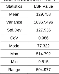
This study begins by analyzing the basic statistics with results obtained from the central and dispersion values of C LSF data. The basic statistics result is shown in table 4.1 below:

TABLE4.1

BASIC STATISTICS RESULT

Statistics LSF Value

Mean 129.758

Variance 16367.496

Std.Dev 127.936

CoV 0.986

Mode 77.322

Max 514.792

Min 9.815

Range 504.977

The results obtained from the statistical analysis shows that large data variations were detected, with varying values of calculated average (Mean) and median, indicating that the data is not normally distributed. The characteristics of the boxplot LSF were studied which showed deviations and abnormalities in the statistical analysis above and below the whisker. The LSF Boxplot graph is seen below (Fig 4.1).

Fig. 4.1. Boxplot LSF

4.2 Fitting Test Chi-Square Method

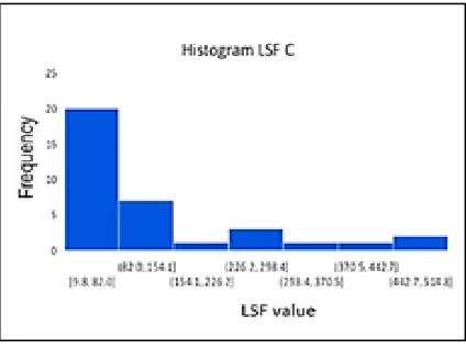
1682 Fig. 4.2. Histogram LSF

From the histogram graph, the most suitable distribution with the LSF data is obtained by comparing the empirical data to the theoretical distribution. Fitting Test is carried out with Matlab software. Fig. 4.3 Below is the Data Distribution graph

Fig. 4.3. Data Distribution

Visually, the log type is normal, and the exponential distribution has a shape that follows the histogram value of the LSF data. However, the Chi-Square calculation needs to be conducted to ascertain the type of LSF distribution. [26] The calculation begins with determining the midpoint value of each histogram bar and comparing the middle values of all data distributed. Chi-Square Method Fitting Test Results are seen in table 4.2 below.

TABLE4.2

FITTING TEST CHI-SQUARE METHOD RESULTS

Value

Distribution Type

Normal Lognormal Exponential Gamma

Mean 129.76 131.26 129.76 129.76

Variance 16367.5 21713.1 16837.1 11982.6

Std.Dev 127.94 147.35 129.76 109.47

CoV 0.98 1.12 1 0.84

Skewness 1.24 1.11 1.22 1.45

Chi-square

0.01590 9

0.0040045 91

0.0033609 48

0.0048133 5

When the chi-square value is small, the theoretical frequency is considered to be observable and is seen accordingly [26]. Therefore, the type of data distribution is referred to as Exponential Distribution.

4.3 Variogram and Cross-Validation

To generate a variogram modeling, it is important to determine the lag distance, the number of lags, and the angle tolerance. [27]. The lag size is determined by the average distance from the space of data collection (boreholes). The number of lags is determined by dividing the farthest distance from the data collection location with the average distance between the data.

The following values were obtained:

• Max Lag Distance = 520 meter • Lag = 40 meter • Number of lags = 520/40

= 13 data pairs • Angle Tolerance = 22.50

• Direction = 1350

The variogram requires a model to estimate the actual data and acquire the optimal Sill, Range, and Nugget Effect values. Variogram fitting was carried out using the trial and error method before the most appropriate model was obtained based on error calculation or error and cross-validation. [28 ],[29] Tables 4.3, 4.4, and 4.5 show the error in the Gaussian, Exponential, and Spherical variogram models. Based on the three models, the smallest error value was then searched. The smallest error value data was used in the subsequent analysis of the variogram model.

TABLE4.3

ERROR VARIOGRAM GAUSSIAN MODEL

Range Sill

30000 35000 40000 45000 50000

150 18.33% 18.3% 18.41% 18.53% 18.63%

175 19.86% 19% 18.39% 17.8% 17.31%

200 23.8% 23.47% 23.1% 22.67% 22.26%

225 23% 23.27% 23.46% 23.58% 23.7%

250 18.92% 19.58% 20.14% 16.63% 21.03%

TABLE4.4

ERROR VARIOGRAM EXPONENTIAL MODEL

Range Sill

30000 35000 40000 45000 50000

150 13.66% 13.65% 13.64% 13.63% 13.63%

175 13% 12.99% 12.99% 12.97% 12.99%

200 12.75% 12.74% 12.74% 12.73% 12.74%

225 12.65% 12.64% 12.64% 12.62% 12.64%

1683

TABLE4.5

ERROR VARIOGRAM SPHERICAL MODEL

Range Sill

30000 35000 40000 45000 50000

150 51.95% 51.92% 51.91% 51.9% 51.88%

175 47.01% 46.98% 46.96% 46.94% 46.98%

200 43.71% 43.68% 43.68% 43.68% 43.68%

225 40.01% 39.98% 39.98% 39.98% 39.98%

250 37.09% 37.07% 37.07% 37.07% 37.07%

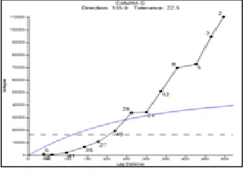
• The error calculation is based on the absolute value of the difference in the estimated variogram and LSF recorded in percents. From the three models analyzed, the smallest error was 12.55% in the Exponential model using the variogram parameters and is stated as follows: Sill: 45000

• Range: 250 meter • Nugget Effect: 100

Fig. 4.4 shows the experimental graph of the LSF variogram that has been modeled with the Exponential Model, therefore, the sill, range, and nugget effect is obtained.

Fig. 4.4. Variogram Model Exponential

Variogram assessment requires the expertise of geostatistics experts, and visually, the model chosen is based on the number of pairs that intersect with the model. However, due to limitations in the study and outlier data from boxplot analysis, the variogram was chosen based on the smallest error. Subsequently, cross-validation was conducted to satisfy the rules of BLUE (Best Linear Unbiased Estimator) in the analysis. [30]. Cross plot showed the alignment of the distribution of points and the values of the observed and estimated data. Cross-validation of the model is shown in Fig. 4.5 for the LSF because the RMSE is closer to zero, fitted Exponential models yielded better results, and was adopted in this study.

Fig. 4.5. Variogram cross-validation

Visible data points evenly spread on the centerline with the distribution of points above and below the line.

5 CONCLUSION

In conclusion, LSF contains outliers obtained from the boxplot and an exponential distribution of the Chi-Square analysis. The most optimal variogram model with the smallest error size is the Exponential variogram model with parameters Sill 45000, Range 250, Nugget Effect 100, and a total error of 12.55%.

6

A

CKNOWLEDGMENT

This research was supported by the Mining Engineering Department, Faculty of Earth and Energy Technology, Universitas Trisakti, Jakarta, Indonesia. Thanks are expressed to PT Indocement Tunggal Prakarsa Tbk. Palimanan unit, Cirebon, and all those that contributed to the success of this research for their support and assistance. Thanks also to the STEEM (Science, Technology, Engineering, Economics, Education, and Mathematics) Conference.

7

REFERENCES

[1]. Aldidamouni Hamdi Ahmed, D. Ahmed Saleh Mohammed Taha (2011) book: Chemistry and Technology cement. [2]. Walter, H. D (1985). Cement Data Book. Weisbaden Berun:

Bauverlag GmBH.

[3]. Rikoto I.I, Nuhu, S (2019). Effect of Free Lime and Lime Saturation Factor on Grindability of Cement Clinker. International Journal of Engineering Research and Reviews ISSN 2348-697X (Online) Vol. 7, Issue 1, pp: (61-66) [4]. Anonymous, (2003), "Company Overview", PT. Indocement

Tunggal Initiative Tbk, Cirebon

[5]. N. H. Mtarfi, Z. Rais, M. Taleb (2017). Effect of clinker free lime and cement fineness on the cement physicochemical properties. Journal of Materials and Environmental Sciences. ISSN: 2028-2508. JMES, 2017 Volume 8, Issue 7, Page 2541-2548.

[6]. Boughanmi, S., Iabidi, I., Tiss, H., and Megriche, A (2016) The Effect of Marl and Clay Compositions on the Portland Cement Quality, Journal of the Tunisian Chemical Society, 2016, vol. 18, pp. 43–51

[7]. Lefond. J. Stanley (1983). Industrial Minerals and Rocks (Nonmetallics other than Fuels). Society of Mining Engineers. New York.

[8]. Rakesh Rana, Richa Singhal (2015). Chi‑square Test and its Application in Hypothesis Testing. Journal of the Practice of Cardiovascular Sciences . Volume 1. Issue 1

1684 properties. Journal of JMES, 2017 Volume 8, Issue 7, Page

2541-2548

[10].Hendrick G van Oss (2012) Cement, Mineral Commodity Summaries, U.S Geological Survey, pp 38-39.

[11].A. C. Ozdemir, A. Dag, and T. Ibrikci (2018). A Comparative Assessment on Cement Raw Material Quarry Quality Distribution via 3-D Identification. Journal of Mining Science, Volume 54, Issue 4, pp 609–616.

[12].Soumaya Ibrahimi, Néjib Ben Jamaa, Mohamed Bagané, Mekki Ben Ammar, André Lecomte, Cécile Diliberto (2015). The Effect Of Raw Material’s Fineness And Lime Saturation Factor On Clinker’s Grindability And Energy Efficiency In The Gabes Cement Industry. Journal of Multidisciplinary Engineering Science and Technology (JMEST)ISSN: 3159-0040. Vol.2, Issue 11.

[13].V.C. Johansen, L.M. Hills, F.M. Miller and R.W. Stevenson (2002). The Importance of Cement Raw Mix Homogeneity, International Cement, Chicago, USA, online on America's Cement (2003)

[14].Rao D.S, Vijayakumar T.V., Prabhakar S, Bhaskar Raju G (2011). Geochemical Assessment Of A Siliceous Limestone Sample For Cement Making. Chin.J.Geochem Chinese Journal of Geochemistry. Volume 30, Issue 1, pp 33– 39.DOI: 10.1007/s11631-011-0484-8. Springer Link

[15].Supardi, U. (2013). Statistics Application in Research. Jakarta: Change Publication.

[16].Junaidi. (2004). Data Description Through Boxplot. Faculty of Economics and Business, University of Jambi.

[17].Marwanza, I., Nas. C, Azizi. A. M, Dahani. W, Subandrio (2019). Geostatistic Application In Determining The Spread Of Claystone Rock Mass Characteristics In Coal Mining. IJSTR Volume 8 - Issue 10, October 2019 Edition - ISSN 2277-8616

[18].Isaaks, E.H., and Srivastaya, R.M (1989). An Introduction To Applied Geostatistics, Oxford University Press: NewYork. 561p

[19].Marwanza, I., Nas, C., Badaruddin, S.P., Azizi, M.A (2018). Copper Resource Estimation in PT X Batu Hijau, Regency of West Sumbawa, West Nusa Tenggara Province using geostatistical method. IOP Conference Series: Earth and Environmental Science

[20].Amine Soufi, Lahcen Bahi and Latifa Ouadif (2018). Contribution Of Geostatistical Analysis For The Assessment Of Rmr And Geomechanical Parameters. VOL. 13, NO. 24, ISSN 1819-6608. ARPN Journal of Engineering and Applied Sciences ©2006-2018 Asian Research Publishing Network (ARPN). All rights reserved.

[21].Bohling, G. (2005). Introduction To Geostatistics And Variogram Analysis, Earth, 1-20.

[22].Zhanglin Lia, Xialin Zhanga, Keith C. Clarkec, Gang Liua, Rui Zhuc. (2018). An automatic variogram modeling method with high-reliability fitness and Estimates. Journal of Computers & Geosciences, 120. DOI: 10.1016/j.cageo. © 2018 Elsevier Ltd. All rights reserved.

[23].Han, C., Wang, J., Zheng, M., Wang, E., Xia, J., Li, G., Choe, S. (2016). New Variogram Modeling Method Using

MGGP And SVR. Earth Sci. India.

https://doi.org/10.1007/s12145-016-0251-9.

[24].Rossi, M.E. and Deutsch, C.V. (2013). Mineral Resource Estimation, Springer, Dordrecht. 332 P.

[25].Suaad Abdel-Mahdi Abd- Nour and Fatima Allawi Abdul sejad (2014). Measure And Compare The Chemical And Physical Properties For Cement In The Laboratory Of Najaf

And Kufa. Journal of Applicable Chemistry, 3 (2): 812-822. ISSN: 2278-1862

[26].Zhanyu Ma, Arne Leijon, and W. Bastiaan Kleijn (2013). Vector Quantization of LSF Parameters With a Mixture of Dirichlet Distributions. IEEE Transactions On Audio, Speech, And Language Processing, Vol. 21, NO. 9, September 2013. DOI: 10.1109/TASL.2013.2238732 [27].Chiles, J.-P., & Delfiner, P. (2012). Geostatistics Modeling

Spatial Uncertainty: Second Edition. New Jersey: John Wiley & Sons, Inc.

[28].Deutsch, J.L., Szymanski, J. and Deutsch, C.V (2014). Checks and measures of performance for kriging estimates, Journal of the Southern African Institute of Mining and Metallurgy, 114:3, 223-230.

[29].Deutsch, J.L., Palmer, K., Deutsch, C.V., Szymanski, J. and Etsell, T.H (2015) Spatial Modeling of Geometallurgical Properties: Techniques and a Case Study, Natural Resources Research, 25:2, 161-181.