Application of The Method of Elastic Maps In Analysis of Genetic Texts

Application of The Method of Elastic Maps In Analysis of Genetic Texts

A. N. GORBAN

Krasnoyarsk, Russia

A. Y. ZINOVYEV

Scientifiques (IHES), Bures-sur-Yvette, France

D.C. WUNSCH

USA

Abstract - Method of elastic maps1 allows to construct efficiently 1D, 2D and 3D non-linear approximations to the principal manifolds with different topology (piece of plane, sphere, torus etc.) and to project data onto it. We describe the idea of the method and demonstrate its applications in analysis of genetic

sequences.2

I.INTRODUCTION

y(i) E(i)(0) E(i)(1) R(i)(1) R(i)(0)

Numerous experimental techniques in modern molecular biology collect huge amounts of information that needs intelligent data mining. The basic property of the information is its multidimensionality. Rather than 2-3 a typical object in database has hundreds and thousands features. Because of this the information loses it’s clearness and one can’t represent the data in visual form by standard visualization means – graphs and diagrams.

R(i)(2)

In this paper a technology of visual representation of data structure is described. Many interesting patterns could be discovered using visual two-dimensional (or three-dimensional) pictures of data and laying on it some additional relevant information. This data image should display cluster structures and different regularities in data.

The basic of the technology that we proposed in Gorban and Zinovyev (2001) is an original idea of elastic net – regular point approximation of a manifold that is embedded into multidimensional space and has minimal energy in a certain sense. This manifold is an analogue of principal surface and serves as a non-linear screen on which multidimensional data points can be projected.

The specialists in different fields can use the technology. We present an example of application of the technology in bioinformatics, where the need of visual data analysis is very necessary.

1

http://cogprints.ecs.soton.ac.uk/archive/00003088/ and http://cogprints.ecs.soton.ac.uk/archive/00003919/

2

The animated 3D-scatters are available on our web-site: http://www.ihes.fr/~zinovyev/7clusters/

II.CONSTRUCTING ELASTIC NET

Method of elastic maps, similar to SOM

(self-organizing maps), for approximation a of cloud of data points uses an ordered system of nodes which is placed in the multidimensional space.

Fig 1. Node, edge and rib

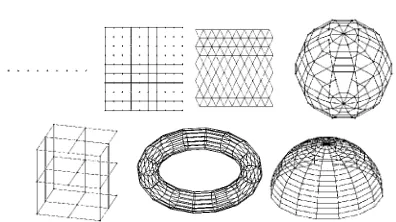
Fig 2. Elastic nets used in practice

Lets define elastic net as connected unordered graph

G(Y,E), where Y = {y(i), i=1..p} denotes collection of

graph nodes, and E={E(i), i=1..s} is the collection of graph edges. Let’s combine some of the adjacent edges in pairs

R(i) = {E(i),E(k)} and denote by R={R(i), i=1..r} the collection of elementary ribs.

Every edge E(i) has the beginning node E(i)(0) and the end node E(i)(1). Elementary rib is a pair of adjacent edges. It has beginning node R(i)(1), end node R(i)(2) and the central node R(i)(0) (see Fig. 1).

forth – non-planar graph whose nodes are arranged on the sphere (spherical grid), then a non-planar cubical grid, torus and hemisphere. Elementary ribs at these graphs are adjacent edges that subtend a blunt angle.

Let’s place nodes of the net in a multidimensional data space. This can be done in different ways, placing nodes randomly or placing nodes in a selected subspace. For example, it can be placed in the subspace spanned by first two or three principal components. In any case every node of the graph becomes a vector in RM.

Then we define on the graph G energy function U that summarize energies of every node, edge and rib:

U = U(Y) + U(E) + U(R). (1)

Let’s divide the whole collection of data points into subcollections (called taxons) K(i), i = 1…p. Each of them contains data points for which node y(i) is the closest one:

( ) ( ) ( )

{ j : j i min

i

Y

K = x x −y → }. (2)

Let’s define ( ) ( ) 2 ( ) ( ) ( ) 1 1 j i p Y

i x K

U x

N = ∈

=

∑ ∑

y

− , (3)

2

( ) ( ) ( )

1

(1) (0)

s

E i i

i i

U λ E E

=

=

∑

2

( ) ( ) ( ) ( )

1

(1) (2) 2 (0)

r

R i i i

i i

U µ R R R

=

=

∑

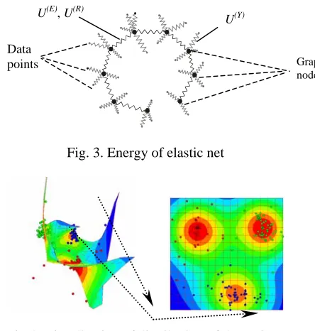
Actually U(Y) is the average square of distance between y(i) and data points in K(i), U(E) is the analogue of summary energy of elastic stretching and U(R) is the analogue of summary energy of elastic deformation of the net. We can imagine that every node is connected by elastic bonds to the closest data points and simultaneously to the adjacent nodes (see Fig. 3).

Values λi and µj are coefficient of stretching

elasticity of every edge E(i) and coefficient of bending elasticity of every rib R(j). In simple case we have

1 2 ... s ( )s

λ =λ = =λ =λ , µ1=µ2 = =... µr =µ( )r .

Simplified consideration shows that, if we require that elastic energy of the net remains unchanged in case of finer net, then

2 0 d d s λ λ= − , 4 0 d d r

µ µ= − (6)

where d is the “dimension” of the net (d = 1 in the case of polyline, d = 2 in case of hexagonal, rectangular and spherical grids, d = 3 in case of cubical grid and so on).

Energy (1) is minimized to get the optimal configuration of nodes. For details of minimization procedure see Gorban et al. (2001), Gorban and Zinovyev (2001). Then the net is used as non-linear screen to visualize distribution of datapoints by projecting them onto the manifold, constructed using the net as point approximation. Then different colorings could be put onto the screen to show any function of coordinates of

dataspace, for example, estimation of density of distribution (see Fig.4).

The method of constructing non-linear principal manifolds is implemented in freely distributed software ViDaExpert, working under Windows and available on the author’s web page:

http://www.ihes.fr/~zinovyev/vida/vidaexpert.htm.

U(Y)

Fig. 3. Energy of elastic net

Fig.4. Visualization of distribution of datapoints, coloring by density.

III. VISUALIZATION OF TRIPLET DISTRIBUTIONS IN GENETIC TEXTS

Genetic text of DNA is a long sequence of letters (nucleotides or base pairs) A, C, G, T. Some subwords of the DNA code biological information, necessary for maintaining cell life cycle, and they are called genes. Areas between genes are called intergenic regions or junk

(though it is not exactly true).

The most of working molecules in a cell are called

proteins and they are composed from aminoacids. The

information that defines the order of aminoacids in protein is coded in DNA by codons – triplets of nucleotides. If we take arbitrary window of coding sequence and divide it into successive non-overlapping triplets, starting from the first base pair in window, then this decomposition and arrangement of the real codons may not be in phase. We can divide the window into triplets in three ways, shifting every time on one base pair from the beginning. So we have three possible triplet distributions and one of them coincides with the real codons distribution. So the coding regions are characterized by the presence of distinguished phase.

Data points

U(E), U(R)

Junk evidently has no such feature because inserting and deleting a letter in junk do not change properties of DNA considerably, thus this kind of mutations is allowed in the process of evolution. But every such mutation breaks the phase, so we can expect than distributions of triplets in junk will be similar for all three phases.

In this section we analyze distribution of triplet frequencies in window of size W, sliding along the whole sequence.

Let us denote triplet frequency distribution by fijk ,

where i,j,k∈{A,C,G,T}, i.e., for example, fACG is equal to the frequency of the ACG codon in a given coding region. We have constructed datasets of triplet frequencies for several real genomes and for several model genetic sequences as follows:

1) Only the forward strands of genomes are used for triplet counting.

2) Every p positions in the sequence, we open a window (x-W/2,x+W/2), of size W and centered at position

x.

3) Every window, starting from the first base-pair, was divided into W/3 non-overlapping triplets, and the frequencies of all triplets fijk calculated.

4) The dataset consists of N = [L/p]points, where L

is the entire length of the sequence. Every data point

Xi={xis} corresponds to one window and has 64

coordinates, corresponding to each frequency of the sth possible triplet.

5) Then a standard procedure of centering and normalization on a unit dispersion is applied, i.e.,

is s is

s

x m x

σ

− =

% ,

where

x

%

1 1 N

s ts

t

m

N =

=

∑

(

)

1 1 N

s ts

t

x m

N

σ

=

=

∑

is the standard deviation of

sth coordinate.

Algorithm of elastic maps was applied for these datasets. Below we present the results of visualization for

Caulobacter crescentus complete genome (GenBank

accession code is NC_002696). Parameters used are

W=300, p=600.

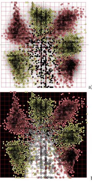
In Fig.5a we presented distribution of data points projections on the elastic map. We made coloring by estimation of point density. One can see clearly that the distribution has 6 well-defined clusters3 and a sparse cloud of points between these clusters. To understand it, we used known annotation of the genome and marked by black circles points, corresponding to non-coding regions;

3

http://cogprints.ecs.soton.ac.uk/archive/00003077/

squares and triangles corresponds to the coding regions, but in different strands of the genome (in bacterial genomes, a gene can be positioned in forward strand or

complementary strand, in the last case it is red in opposite

direction and consist of complementary letters G⇔C, T⇔A).

On the early stages of solving task of computational gene recognition (see, for example, Ficket, 1996), many statistics, locally defined on DNA text, were compared by means of application of linear discrimination analysis (two classes – coding and non-coding were separated). On Fig.5b we made coloring by value of linear discriminate function. White color corresponds to the non-coding regions. One can see that linear discrimination in this case make a lot of false positive errors (many non-coding regions are predicted to be coding). More subtle analysis shows that linear discrimination is not appropriate in this case.

a)

b) Fig. 5. Visualization of DNA triplet frequencies

in sliding window. a) point density coloring; b) coloring by linear discrimination function

a)

b) Fig. 6. Visualization of DNA triplet frequencies

in sliding window.

a) coloring by TAA (stop codon) frequency; b) coloring by ATT (complemented stop codon)

frequency.

IV. CODON USAGE EXPLORATORY STUDY

As we mentioned, some parts of DNA texts encode templates, using which, all proteins in a cell are constructed. These parts are called genes. Elementary word in such a template is codon – three genetic letters. There is a map between all possible 64 codons and 20 aminoacids, from which proteins are constructed. In nature this is done by big biological molecule called ribosome – it reads sequence of codons, and link aminoacids in the order encoded by the sequence. This process is called

translation.

genes with much higher frequency then other their synonyms. This phenomenon is known as codon bias. There could be several reasons for explaining codon bias. For example, codon bias can exist because some letters of genetic text must be more frequent then others (for example, letters G and C can be very different in their frequencies then A and T).

In fast growing bacteria codon bias is often connected with translational efficiency [5]. It means that not all codons are translated by ribosome with the same speed. As a result, some codons are preferred in those genes that encode proteins that must be produced at a high speed and quantity in a bacterium. For example, ribosome itself is such a protein, cell should have many of ribosomes, and, therefore, most of ribosomal components are encoded in DNA with “fast” codons.

We are going to apply method of elastic maps to investigation of frequencies of codons in genes – so called

codon usage. As in previous section, every gene is

represented as a 64-dimensional vector with components, corresponding to frequencies of all possible codons.

As our objects, we selected two very famous bacteria: Escherichia coli (GenBank accession code is NC_000913) and Bacillus subtilis (GenBank accession code is NC_000964).

Using known annotations of these genomes, we extracted all protein-coding gene sequences from these genomes. There were 4289 marked genes in Escherichia coli and 4100 in Bacillus subtilis. Tables of frequencies of codons for every gene were used to visualize codon usage for both organisms, using elastic maps method.

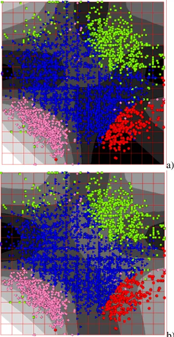
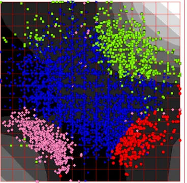
On Fig.7 codon usage of Escherichia coli is presented. Forms of the points correspond to the K-Means clustering into 4 clusters, performed in 64-dimensional space. The background coloring represents density of points. Let us call triangles as genes of class I, circles as genes of class II, squares as genes of class III, and rhombs as genes of class IV.

Comparing the picture with data known from literature on codon usage in different genomes [5-8], we can conclude that class I contains most of genes with very diverse functions. Class II contains genes that are highly expressed in a cell (present in large quantities). Class III contains genes with unusual (non-specific for a given genome) codon usage. Often these genes are suspected to be transferred from other organisms (horizontal transfer

phenomena). Finally, genes in class IV encode proteins which are considerably different in their aminoacids composition from the rest of proteins. Namely, these proteins contain many highly hydrophobic aminoacids (like leucine and phenylalanine) and small number of hydrophilic aminoacids (like arginine and glutamate).

To demonstrate how useful the display constructed with method of elastic map could be, let us give some examples.

Fig. 7. Codon usage of Escherichia coli. The gray coloring shows density distribution.

a)

b) Fig. 8. Codon usage of Escherichia coli. The coloring a) shows frequency of GAA codon;

Fig. 9. Codon usage of Escherichia coli. The coloring shows GC-content of genes.

Fig. 10. Codon usage of Bacillus subtilis. The gray coloring shows density distribution. It is known that glutamate aminoacid can be encoded in genes with two codons: GAA and GAG. Figure 8a and 8b show colorings corresponding to the frequencies of these two codons. It is clear that class IV lacks this type of codons (as we mentioned, class IV is glutamate-poor). Also we can conclude that part of genes in class II uses much more GAA codons than GAG, but this is not so contrast in the genes of class I. This means that GAA codon is translationally preferred in comparison with GAG codon.

Other important characteristic of codon usage is GC-content of a gene (relative percentage of G and C letters in a gene). It is clear that GC-content is a simple linear function of codon frequencies. On Fig. 9 this function is represented. It is clear that class III of genes is very

different from others in it’s GC-content (it is GC-poor or AT-rich in comparison with all other classes).

Figure 10 represents visualization of codon usage of Bacillus subtilis. The pattern of codon usage in this case is very similar to E.coli bacterium. Indeed, they are both fast-growing bacteria with similar fast-growing conditions.

V. CONCLUSION

In this paper we described method of elastic maps for constructing representations of experimental data-tables in visual form. These representations may give insight to how data should be treated and what quantitative methods might be applied. Besides, informative pictures of data give possibility to control process of data analysis and make it more reliable.

The purpose of this method (with respect to applications in data visualization) is to provide more informative data visualization displays that are suitable for visualizing not only data points but also informative layers of related characteristics. With increasing number of experimental datasets in such fields as molecular biology, the need in such tools will grow continuously.

As it has been demonstrated, the method allows discovering interesting patterns in large datasets, such as tables of local triplet frequencies for long genetic texts or codon usage tables.

REFERENCES

[1] Gorban A.N., Pitenko A.A., Zinov'ev A.Y., Wunsch D.C. 2001. “Visualization of any data using elastic map method.” Smart Engineering System Design, V.11, p. 363-368.

[2] Gorban A.N., Zinovyev A.Yu.2001. “Visualization of Data by Method of Elastic Maps and Its Applications in Genomics, Economics and Sociology.” Institut des

Hautes Études Scientifiques preprint. IHES/M/01/34,

2001

[http://www.ihes.fr/PREPRINTS/M01/Resu/resu-M01-34.html]

[3] Gorban A.N., Zinovyev A. Yu. Method of Elastic Maps and its Applications in Data Visualization and Data Modeling // International Journal of Computing Anticipatory Systems, CHAOS. 2001. V. 12. PP. 353-369.

[4] Fickett J.W. 1996. “The Gene Identification Problem: An Overview For Developers.” Computers Chem., Vol.20, No.1, pp.103-118.

[5] M. Gouy, Ch. Gautier. Codon usage in bacteria: correlation with gene expressivity. Nucleic Acids

[6] I. Moszer, E.P.C. Rocha, A.Danchin. Codon usage and lateral gene transfer in Bacillus subtilis. Current

Opinion in Microbiology, 2:524-528, 1999.

[7] P.M. Sharp, E. Cowe, D.G. Higgins, D.C. Shields, K.H. Wolfe, F.Wright. Codon usage patterns in Escherichia coli, Bacillus subtilis, Saccharomyces cerevisiae, Drosophila melanogaster and Homo

sapiens: a review of the considerable within-species

diversity. Nucleic Acids Research, 16:8207-2811, 1988.

[8] C. Medigue, T. Rouxel, P. Vigier, A. Henaut, A. Danchin. Evidence for horizontal gene transfer in

Escherichia coli speciation. Journal of Molecular