Development Of A Scoring Model For Determining The Probability Of A Delay In Lease Payments By The Lessee

1995

Development Of A Scoring Model For

Determining The Probability Of A Delay In Lease

Payments By The Lessee

Irina Ivanovna Glotova, Elena Petrovna Tomilina, Lyubov Vasilevna Agarkova, Yuliya Evgenevna Klishina, Olga Nikolaevna Uglitskikh

Abstract: An analysis of the current situation in the leasing services market has shown that the change in leasing interest rates is much more frequent than the change in loan rates that vary, as a rule, only if they are tightly linked to refinancing rates. Determining the probability of the lessee default is the main task, which can be followed by risk assessment and further related measures. In order to solve the problem of determining the probability of late payments by the lessee in the modern Russian leasing market with the growing trend towards retail, it was suggested to use the mathematical modeling method based on historical data on the lessees and their behavior.

Index Terms: leasing services, lessee default, risk assessment.

————————————————————

1 I

In order to form a risk management system, there is a need to completely abandon the long-established postulate that the purpose of risk management is to minimize risks, since it leads to the so-called "vicious circle of risk" [9]. Thus, the task of risk management at the level of the leasing company will be to find the optimal ratio between risk and profitability on the scale of both a single leasing transaction and the entire company. At the same time, this optimal ratio should provide both a certain profit level of the leasing company and a risk level not exceeding a certain value, in order to exclude the risk of bankruptcy of the leasing company, which may be the result of one or several risks. Following from this, the risk management of the leasing company is a continuous process consisting of a certain sequence of actions that are repeated throughout the entire life cycle of the company, contributing to the preservation of its financial stability and leveling the negative impacts of external and internal factors. An analysis of the current situation in the leasing services market has shown that the change in leasing interest rates is much more frequent than the change in loan rates that vary, as a rule, only if they are tightly linked to refinancing rates.

Leasing interest rates are more susceptible to the influence of external sources – changes in market rates and in the financial state of the lessee. At the same time, studying the cases of leasing companies' revisions of leasing interest rates allowed us to make an assumption about the reverse dependence of the probability of the lessee default and the likelihood of lowering the leasing rate. If the financial condition of the lessee, which is characterized by a decrease in the probability of default, changes, the leasing company could enter into a contract at a lower rate, which may serve as an excuse for applying to the leasing company in order to reduce the rate. On the other hand, this may also cause a drop in market rates, even with the financial state of the lessee unchanged.

2 R

D

Determining the probability of the lessee default is the main task, which can be followed by risk assessment and further related measures. In order to solve the problem of determining the probability of late payments by the lessee in the modern Russian leasing market with the growing trend towards retail, it was suggested to use the mathematical modeling method based on historical data on the lessees and their behavior. With regard to expert opinions on credit risk assessment as well as the methodology proposed by N. Siddiqi [10], the process of creating a scoring model for estimating the probability of past-due payment by the lessee was determined. The first step is to define the objectives of the project from the point of view of the organization. The retail leasing company in the Russian market may use the following set of goals:

1. Decrease in the number of debts that result in the

lessee defaults.

2. Increase in the profitability of the leasing company.

3. Decrease in the cost of processing leasing applications

by automating decision-making based on the scoring model.

4. Increase in the predictive power compared to the

scoring card of the credit bureau used in the leasing company as an external decision-making tool. ___________________________________

 Irina Ivanovna Glotova – Associate Professor at the Department of "Finance, Credit and Insurance" in Federal State Budgetary Educational Institution of Higher Education «Stavropol State Agrarian University», Russian Federation

 Elena Petrovna Tomilina – Associate Professor at the Department of "Finance, Credit and Insurance" in Federal State Budgetary Educational Institution of Higher Education «Stavropol State Agrarian University», Russian Federation

 Lyubov Vasilevna Agarkova – Professor at the Department of "Finance, Credit and Insurance" in Federal State Budgetary Educational Institution of Higher Education «Stavropol State Agrarian University», Russian Federation

 Yuliya Evgenevna Klishina – Cand. Sc. (Economics) at the Department of "Finance, Credit and Insurance" in Federal State Budgetary Educational Institution of Higher Education «Stavropol State Agrarian University», Russian Federation

1996 At the data analysis stage, the issue of data accessibility for

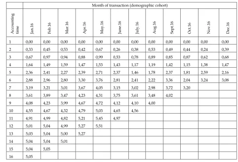
constructing a scoring model in terms of quality and quantity is considered, since only reliable and clean data are required with a minimum allowable number of entries for each target event. The amount of data needed may be different, but in general it must meet the requirements of statistical significance and randomness. When identifying the project parameters, one should first exclude some types of clients from the training model sample, namely those characterized by a nonstandard position relative to other client categories (e.g., VIP clients). Then it is necessary to determine the exponential period and the "sampling window", as the statistical model is based on the assumption that the future is a reflection of the past. Thus, there is a need to collect data on customers who took transport/special equipment in leasing for a certain period of time and determine whether these lessees were in default for another time interval. The exponential period covers the period of time during which the client's behavior is monitored for a certain period (i.e. within the "sampling window") and assigned to a particular class [10]. The "sampling window" specifies the time interval for which the known "default" or "no default" cases will get into the training sample. Table 1 provides an analysis of the demographic cohorts to determine the client with a delay of 60+ days and a 16-month exponential period. The last figure in each column shows the current status of the delay and should be used as data for analysis. These figures show the share of clients of the leasing company with arrears after a certain number of months.

Table 1. Analysis of the demographic cohorts of the sample of clients of the leasing company, %

Figure 1 shows the portfolio of one of the surveyed leasing companies. It reflects changes in the clients with a delay of 60+ days in the mature cohort of January 2016 by the months of issuing a loan from the leasing company for a period of 16 months.

Figure 1. Dynamics of defaulted lessees. Note: Месяц – Month

Figure 2 shows that the level of the defaulted lessees increased rapidly in the first months, and then stabilized as the service life in the leasing company approached 12 months. Thus, the "sampling window" for the leasing company will be between 12 and 14 months, i.e. the exponential period covers on average 13 months. The training sample from the mature cohort is taken in such a way as to minimize the misconceptions of client behavior. After the client’s negative target behavioral attribute (a delay of 60+ days in our case) is determined, it is necessary to determine the client’s positive target attribute. A "good" client is one who has had neither a 60+ delay nor a 10+ delay. It should be taken into account that we will have an "undetermined" class of clients, i.e. those who cannot be classified as either positive or negative. For example, these are clients with the insufficient history in the leasing company or with a delay of more than 10 days, but less than 60. For qualitative analysis, the "undetermined" clients

should not be more than 10-15% of the portfolio. Their inclusion in the training model sample can lead to an erroneous classification, which is why we will not consider them in this study. Having determined the project parameters, one should create a database for constructing a scoring model. The selection of predictive characteristics for inclusion in the sample is one of the important parts of the development process. We have formulated the criteria that should guide the preliminary selection of predictors:

1. Predictive power based on experience and business

knowledge.

2. Convenience of data collection with the existing

business process in the leasing company.

3. Reliability (impossibility of rapid falsification).

4. Interpretability.

5. Longevity and future availability.

A number of studies of the methods of assessing the financial and economic activities of the lessees used by leasing companies and banks in practice [2; 3; 5; 9; 11; 12; 13] showed that the number of ratios used for the analysis ranges from 2 to 67. However, in the Russian context it is impossible to draw a conclusion about the lessee’s financial state only on the basis of the official data of the lessee's own reporting. Accordingly, in our opinion, it is not appropriate for the Russian reality to construct a model based on statistical methods, using only financial ratios as predictors [6;7]. Moreover, the goal of developing a scoring model is to determine the most complete risk profile of the client. This approach not only increases the predictive power of the model, but also makes it more stable under changing conditions. This once again confirms the fact that the risk profile should include features from as many types of data as possible.

Thus, the following aspects should be taken into account in the model:

1. Financial ratios of the lessee's activity.

2. Data of credit bureaus (CB) on the payment discipline

of the lessee as a legal entity as well as individuals-owners of the company/group of companies.

3. Behavioral data of the lessee, i.e. the history of the

relationship with the lessor company.

In order to determine the set of financial ratios used to analyze the lessee’s activities, based on the described techniques as well as conversations with top managers of one of the leasing companies studied, we identified the ratios that are most often used to assess the financial and economic activities of the lessee. Below are the ratios mentioned in more than 50% of the techniques studied, in descending frequency of application:

1. Current liquidity ratio

2. Quick (acid) liquidity ratio

3. Absolute liquidity ratio

4. Net profit margin ratio

5. Equity ratio

6. Working capital to current assets ratio

7. Profit margin ratio

8. Return on equity

1997

10. Equity flexibility ratio

11. Return on assets

12. Asset turnover ratio

13. Debt to equity ratio

However, at the current stage of Russian business development, one cannot draw accurate unambiguous conclusions about the financial state of the lessees solely on the basis of their reporting indicators. In addition, despite the successful experience of many banks in managing credit risk based on the use of statistical models of assessing the probability of the borrower’s default, the problem of the lack of data on credit history for the formation of predictors remains relevant. Not all credit institutions have sufficiently complete qualitative data on the payment discipline of their borrowers. In this regard, the client company may have credit obligations to other leasing companies, banks, suppliers of equipment, goods, etc. With the development of CB services, banks were the first to use aggregated data on the payment discipline of borrowers in the form of a CB score. Thus, the problem of combining the borrower's risk assessment based on the questionnaire parameters (coefficient scoring, in our case) and the borrower's risk assessment based on the credit history (CB scoring) becomes urgent. CBs currently aggregate a lot of information on transactions related to debt servicing, which allows using an array of data that is not available to financial organizations for creating models due to the limited input data flow. It is cheaper for the company to use these data in the form of scoring than to obtain a credit report. In terms of their predictive power, behavioral data are more important than the demographic characteristics of the questionnaire scoring, since they are closer to the actual behavior of the organization/person in relation to debt servicing than the variables determined by the company's balance sheet, geography, business sector etc. By adding data on the CB score to the model built on the basis of internal characteristics and behavioral data accumulated by the leasing company, the efficiency of the forecast of estimating the probability of arrears will increase. When including the CB data in the scoring model of the leasing company, one should exclude a possible correlation of predictors. The internal model does not need to include the variables based on the data used by CBs for constructing their models, for example, by the internal payment discipline, because they are already included in the calculation of the CB score. The CB scoring card is based on the customer's transaction data following the credit history, such as the number of loans, the dynamics of repayment, the occurrence of delays, the depth of delays, the observance of maturities, the utilization of credit limits, the length of credit history, and other aggregates related to debt servicing, which are contained in the CB. This means that such a card is a behavioral scoring estimate. Particular attention should be paid to the use of CB scoring estimates in the development of the internal model. A natural limitation in the compilation of an integral measure of evaluation is the simplicity, speed and convenience of combining the estimates obtained on the basis of the internal and external (one or several) models. It is necessary to ensure such a combination of estimates, in which changes in one of the estimates will not

require the restructuring of the entire evaluation strategy. The construction of a combined estimate consists of several stages: to prepare a sample for retro-scoring, which can help evaluate the quality of the model for a particular leasing company, to analyze the results of the CB retro-scoring, as well as to choose a way of combining external and internal estimates. There are several methods for constructing an integrated evaluation system. In the context of a consistent strategy, the applicant, who has not passed a certain stage, does not pass to the next one. In the context of a consistent approach, the client is evaluated first by the questionnaire scoring, then – by the CB scoring. Those clients who get a lower score by the first model are eliminated, and the system ceases to operate with respect to them. In the context of a matrix approach, the elements of a common evaluation system function together, and there is a compromise between the forecasts of its individual parts. For example, the customer can get a low score by one of the scoring models and a high score – by the other; the overall evaluation in this case will be satisfactory [8]. It is often recommended to build decision matrices, where the rows are the intervals of one scoring value, and the columns are the intervals of another scoring estimate. The cells calculate the probability of the occurrence of a target delay in the group of customers with a certain combination of estimates for the two models. In practice, it may turn out that in order for each cell to be filled, scoring points will need to be divided into large intervals – thus the accuracy of evaluation may be significantly reduced. If the intervals are too small, there may not be enough data at the intersections of the intervals. Similarly, if there are more than two estimates, the matrices are once more complicated and they must be aggregated in other ways [4]. After analyzing the ways of combining the estimates of different models, we suggest using a weighted average of the estimates. This approach is easily interpreted and implemented. By using certain variables in the formula, we can easily manage it in the event of a decrease or, on the contrary, an increase of confidence in any of the models involved in the calculation, as well as in the case of adding the models to the combined estimate. Due to the above peculiarities of using the CB scores in the evaluation of the lessees, we will add these data to the model after building an internal model based on financial coefficients and behavioral data within the leasing company. By using the behavioral data of the lessee that reflect the history of the relationship with the leasing company and interviewing the top managers of one of the leasing companies studied we identified those that must be included in the set of predictors when building the model and, at the same time, that are not used in building the CB scoring:

1. The number of the lessee’s previous transactions with

this leasing company.

2. The main subject of leasing, acquired by the lessee

from the leasing company (according to the European classification of vehicles and special equipment).

3. The duration of the relationship of the lessee with the

leasing company.

1998 control (test) one, based on which the model will be checked.

Typically, 70-80% of the sample is used to develop the model, and 20-30% – to test it. The question remains what percentage of positive and negative borrowers should be included in the total sample. Usually, for the development of a scoring model, an excessive sample is used (the shares of "good" and "bad" borrowers in the training sample are different from the shares in the actual population), as it reduces the influence of multicollinearity and allows obtaining a statistically significant result of logistic regression [1]. Excessive sampling is a standard method of predictive modeling, especially when modeling unlikely events. In this case, the training sample requires making a correction for a priori probabilities, i.e. "factoring", in order for the distribution of "good" and "bad" borrowers to be statistically corrected in such a way that their shares reflect the corresponding shares in the actual population. Of the two main methods of correction for the excessive sample, a bias method is recommended to construct a predictive model for the probability of delays, since it is more suitable for the task being investigated, which is precisely described by the logistic model. We will apply the bias method to the training sample before modeling using the proc logistic function in RStudio. Prior to modeling itself, one must use simple statistics to analyze the integrity of the data, as well as their interpretability. This analysis is essential since most financial data have missing values or, conversely, values that are non-relevant for a particular characteristic – these can be incorrectly entered data or outliers. Logistic regression, in contrast to indifferent algorithms, requires that the data sets be complete. Accordingly, these omissions may be processed in the following ways:

1. To exclude all the rows with missing values. The

disadvantage is that in the case of financial data such a method will yield very little data for processing at the output.

2. To exclude characteristics or entries for which the

percentage of missing values is significant (more than 50%) from the training sample. The remaining should be filled with statistical methods (average, median, mode-based, predictive values based on data from other characteristics, etc.).

3. To fill all the omissions with statistical methods.

4. To include all characteristics and entries with missing

values in modeling, assigning special values to the omissions so that they can be read by the algorithm as a separate attribute.

Methods 1-3 assume that missing values carry no additional information, which is not necessarily the case: they may be part of the trend, be associated with other predictors, or be indicators of the client's "bad" behavior. In any case, one should analyze the omissions first, find out whether they are random and neutral from the point of view of the client's behavior, and only after that choose the way to eliminate them. After predictors are treated and preprocessed, it is necessary to identify their correlation both with each other and with the dependent variable, that is, with the probability of a delay of 60+. This step is mandatory and allows excluding the interdependent features, and when making a decision

whether to exclude one of the correlated features, following the degree of their influence on the target event. By using the RStudio statistical package and the function cor(x), a correlation analysis was performed. With regard to the adopted gradation of measures for the strength of linear relationship, according to which the correlation 0.1-0.3 is defined as weak, 0.3-0.5 – moderate, 0.5-0.7 – noticeable, 0.7-0.0.9 – strong, and 0.9-0.99 – very strong, the following features were excluded from the ones previously selected for modeling:

- the profit margin ratio, as it has a correlation with the net

profit margin of sales;

- the return on equity, as it has a high degree of correlation

with the net profit margin of sales;

- the return on assets due to a high degree of connection

with the equity ratio;

- the quick liquidity ratio, as it strongly correlates with the

asset turnover ratio and with the net profit margin of sales;

- the absolute liquidity ratio due to a high degree of

connection with the short-term liabilities turnover ratio;

- the equity flexibility ratio, as it strongly correlates with

the current liquidity ratio and with the working capital to current assets ratio;

- the debt to equity ratio, due to a high degree of connection

with the equity ratio.

Despite a high degree of correlation between the current liquidity ratio and the working capital to current assets ratio (0.85), we defined both ratios as the ones that most fully characterize the company's activities. However, the lessee’s characteristics, which remained as predictors for the scoring model after the correlation analysis, reflect neither the cash coverage of the lessee's obligations, nor the actual efficiency (profitability) of activities, since many companies understate the size of the balance profit in order to optimize taxation. Thus, in the system of variables we have also introduced the ratio of payments on concluded leasing and credit contracts to the company's revenues that most fully reflects the ability of the lessees to fulfill their obligations to pay leasing and credit payments at the expense of revenues from current activities. In addition, if the company's cash turnover is less than revenue, it is recommended that this ratio be supplemented with a coefficient calculated as the ratio of money turnover to revenue. As a result of the transformations, we obtained a system of predictive characteristics for the scoring model to assess the state of the lessee, namely, the probability of a delay of 60+ days (Table 2).

Table 2. The system of characteristics selected for constructing an internal scoring model

1999 particular result. The logit-transformation equation of the

probability of an event looks as follows:

(1) where is the a posteriori probability of a target event with the initial data;

is input variables;

is the segment cut off by the regression line on the axis; is parameters.

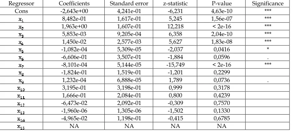
Logit-transformation is the logarithm of chances, namely the logarithm of the relationship between the probabilities of the occurrence and non-occurrence of a target event. To determine the best model using all available options, the method of all possible regressions is used. However, it requires a large amount of calculations, especially if there are many predictors. In practice, in order to build the best model from the available characteristics, we propose using a step-by-step method of logistic regression. This method dynamically adds and removes characteristics from the model at each step, until the best combination is achieved [10]. By using the logistic regression function glm in the RStudio package, based on the prepared training sample, a preliminary scoring model was developed for calculating the probability of a 60+ delay for the lessee. The result of the algorithm is shown in Table 3. The feature is taken as the base variable in the category decomposition of the characteristic ―The main leasing subject acquired from a leasing company (according to the European classification of vehicles and special equipment)‖.

Table 3. The result of logistic regression tested on the prepared database

The significance codes in the form of asterisks in the RStudio package are interpreted as follows:

1. If the P-value is <= 0.001, the significance of the

predictor is very high (***).

2. If the P-value is in the range from 0.001 to 0.01

(inclusive), the significance of the predictor is high (**).

3. If the P-value is in the range from 0.01 to 0.05

(inclusive), the significance of the predictor is normal (*).

4. If the P-value is in the range from 0.05 to 0.1

(inclusive), the significance of the predictor is insignificant (.).

5. If the P-value is in the range from 0.1 to 1 (inclusive),

the significance of the predictor is very low ( ).

After applying the step-by-step selection function of the optimal set of predictors stepAIC in the RStudio package, the final internal scoring model was developed (Table 4).

Table 4. The result of logistic regression tested on the prepared database after the application of stepAIC

Thus, the formula of the internal scoring model in the system of Microsoft SQL Server 2014, which was at the disposal of the studied leasing company and which helped to prepare the database, can be written in the following form:

exp(2,621+1,028* +2,141* +0,00614* +0,01419*

0,0001021* 0,6455* 0,0008187* +0,0001308*

-0,000001994* )/

(1+exp(2,621+1,028* +2,141* +0,00614* +0,01419* 0,0001021* 0,6455* 0,0008187* +0,0001308*

-0,000001994* )) (2)

The most important indicator of the efficiency of a scoring model is its predictive power. It can be calculated using the following statistical methods:

1. The Akaike information criterion (AIC), according to

which penalty points are assigned to the model for adding new characteristics. The smaller the AIC, the better.

2. The Schwartz Bayesian criterion (SBC), which also

assigns penalties to the model for adding new parameters. When creating a scoring model for evaluating risk profiles with the use of the above methods, the AIC and SBC criteria will not be suitable for accurately determining the predictive power of the model. The reason is that when developing the risk profile of the lessee, we chose to build a comprehensive estimate of the probability of a delay, that is, in our case the set of predictors is large and does not need to be minimized.

3. The Kolmogorov-Smirnov criterion (CS criterion),

which determines the maximum vertical difference between the total distributions of "good" and "bad" lessees. The downside of this method is that the difference is measured only at one point, not over the entire range of calculated probabilities, and this point may not coincide with the cutoff level.

4. The C-statistic method is the most powerful

nonparametric criterion. It is equivalent to the area under the ROC curve (AUC), the Gini coefficient. This method makes it possible to measure the behavior of the classifier in all ranges and is recognized as the best measure of the predictive power of the model [10]. In the C-statistic method, the AUC of the dependence of sensitivity on (1-specificity) is measured for the entire estimated range. Sensitivity is the ratio of truly positive events (approval of "good" events) to the total actual number of positive ones. Specificity is the ratio of truly negative events (deviation of "bad" events) to the total actual number of negative ones. In order for the sample processed by the scoring model to be better than the random sample, the C-statistic indicator should be greater than 0.5. The value 0.7 and above is considered to be adequate.

2000 Figure 2. The ROC curve of the scoring model for determining

the risk profile of the lessee

In order to control the developed model, we compare the distributions of positive and negative target events between the training and test samples. Figure 3 compares 30% of the control sample and the training sample.

Figure 3. Control chart of the scoring model

The model can be applied to the target population if both data sets are slightly different, as in the presented chart. To do this, it is sufficient to visually compare the curves. Thus, the internal scoring model can be applied in practice to the target population. In accordance with the hypothesis put forward in this section that the addition of data on the CB score to the model constructed from the internal characteristic and behavioral data accumulated by the leasing company will increase the efficiency of the forecast of estimating the probability of past-due payment, we will make a combined estimate of the occurrence of a target event by using CB scores as well as analyze the results of adding the CB data. The first stage of development of the combined model is retro-scoring. Retro-scoring is the calculation of a scoring estimate at a certain point in the past. The value of the score is calculated at the time the financial company makes a decision to issue credit. The data obtained in this way can be compared with the actual behavior of the borrower, revealed by the results of the interaction of the leasing company and the lessee, in order to assess whether the CB score in relation to the specific portfolio of the leasing company was correct and what the real efficiency of its scoring is. Then, we should check the quality of the CB scoring estimate based on the portfolio of one of the large retail leasing companies under consideration. In order to obtain an unbiased estimate, the data set for the analysis should include data of not only those customers whose financing was approved by the leasing company, but also those who were denied. Retro-scoring is limited in terms of the time of calculating scores, each of the CB sets its rules in this regard. Using data from one of the four major bureaus (the National Bureau of Credit Histories, Equifax Credit Services, the United Credit Bureau, the Russian Standard Credit Bureau), who have 95% of the histories with which the leasing company is working, we received the data of retro-scoring on the prepared sample of the lessees (13,873 entries) as of 12 months ago from the current date. The results are shown in Table 5.

Table 5. Aggregated retro-scoring results based on the prepared sample of lessees

Estimate calculated for the lessees Hit rate

11,556 83,3%

The hit rate determines the number of entries from the prepared set on which the score in each of the CB was calculated. It is quite high in the chosen credit bureau. The CB scoring cannot be carried out for all entries in the sample prepared by the leasing company, since the credit history for

calculation may be too small or unavailable at the time the application was submitted (this may be the first application to

a financial company). With the help of the C-statistic indicator,

which, as defined above, is most suitable for estimating the predictive power of the scoring model, we will check the CB estimates. Our example considers only the KGB (Know Good Bad), that is, a censored set of the lessees, and does not take into account the effect of the initial denials, which affects the predictive power of the model because the actual content of the defaults of the incoming flow is underestimated by the denials initiated by the rules for evaluating the lessees that existed at that moment in the leasing company. Therefore, the values of the calculated ratios are understated relative to the actual indicators (Table 6).

Table 6. C-statistic indicators for internal and CB evaluation

Model C-statistics

Internal model 0,75 CB model 0,78

Although the calculated C-statistic indicator for the CB model is higher than for the internal model, but it is still not high enough. This is primarily due to the fact that the data were previously censored as well as limited in size. Nevertheless, the improvement of the predictive qualities of the combined

model will also be noticeable for these data. It is also interesting

to compare the internal model and the CB model by the cumulative distribution: the better the quality of the model, the less the number of "good" borrowers will be cut out by the model with the approval of 50% of the "bad" ones (Table 7).

Table 7. Cumulative distribution of "good" and "bad" lessees

Model Cumulative percentage of _{"bad" borrowers} Cumulative percentage of _{"good" borrowers} Internal

model 50,07 20,20

CB model 50,04 21,72

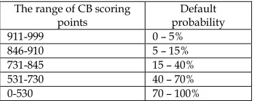
In order to construct a combined estimate of the lessees, one needs to have estimates based on their own internal model and CB data at the time of decision making, rendered into a single value – in our case, the probability of the target event (delay). Table 8 shows the results of calculating the probability matrix in accordance with the CB score ranges.

Table 8. The matrix of default probabilities in accordance with the range of CB points

The range of CB scoring

points probability Default

911-999 0 – 5%

846-910 5 – 15%

731-845 15 – 40%

531-730 40 – 70%

0-530 70 – 100%

2001 range of scoring points. In the considered CB, the scoring

results range from 0 to 999 points:

- 911-999 points. Very good scoring. The probability of a

denial is extremely small.

- 846-910 points. Good scoring. There are good chances of

getting a loan.

- 731-845 points. Average scoring. Getting a loan is

possible, but not guaranteed.

- 531-730 points. Poor scoring. The probability of getting a

loan is extremely small.

- 0-530 points. Very poor scoring. Getting a loan is almost

impossible.

Having received an estimate at the time of making a decision in the past, we will construct a combined estimation model using the weighted average of the estimates. This approach, as mentioned above, is easy to implement and interpret. The weighted average for the two estimates is calculated by the formula:

(3)

where is the weighted average estimate;

w

w

is the value of the first scoring probability estimate;

is the value of the first scoring probability estimate.

Take the weight coefficients as a unity. Having calculated the values in this way, by using the probabilities of one’s own internal model and CB model, we compare the C-statistic indicators (Table 9):

Table 9. C-statistic indicators for internal and CB evaluation

Model C-statistics Internal model 0,75 CB model 0,78 Combined model 0,82

The C-statistic indicator was significantly increased when using the CB scoring points. Obviously, we were able to obtain even higher values of the coefficients of the combined model. Thus, the use of the CB scoring point can greatly enrich the

data and improve the quality of the estimation. Figure 4 shows

the cumulative distribution of "bad" and "good" accounts by the interval of the weighted average value of the estimate. Figure 4. Cumulative distribution of "bad" and "good" lessees by the interval of the weighted average value of the estimate The further construction of the combined estimates is seen in the inclusion of the CB scoring points in the weighted average estimate for individuals-owners / general directors of the lessees. To make a conclusion about the applicability of the received combined

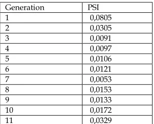
estimate of the lessees, the population stability index (PSI) was calculated by generations of the receipt of the lessees’ applications. The PSI index is calculated to check the sustainability of the scoring estimate. It shows the magnitude of deviation in the population between the new data and the training sample on which the model was built:

(4)

where is the shares of potential lessees in the

corresponding ranges of the estimate values for the considered period;

is the shares of potential lessees in the corresponding ranges of the estimate values for the reference period.

is calculated from the training sample. In our case, the calculation of the index was carried out for all the lessees, which made it possible to calculate the weighted average estimate. The index was calculated for each generation separately (Table 10).

Table 10. Population stability index by generations of the receipt of the lessees’ applications

Generation PSI

1 0,0805

2 0,0305

3 0,0091

4 0,0097

5 0,0106

6 0,0121

7 0,0053

8 0,0153

9 0,0133

10 0,0172

11 0,0329

It can be seen from the calculations that the PSI index did not exceed 0.1 in each of the generations, which indicates that there are no significant changes. This means that the constructed combined model can be applied on the existing incoming flow of potential lessees without the risk of the biased estimation.

5

C

2002

R

[1] C.H. Achen, Interpreting and Using Regression, CA:

SAGE, 1982.

[2] N.Ya. Bambayeva and A.S. Sorokin, Application of

the laws of distributing random variables for the modeling of economic phenomena and processes, Moscow: MESI, 2010.

[3] A. Yu. Belikov, Risk theory. Irkutsk: ISEA, 2001.

[4] I.S. Korchagin, ―The use of CB scores in the

application scoring‖, Risk Management in a Credit Institution, No. 3, pp. 15-19, 2013.

[5] A.V. Lukashov, ―International corporate finance and

management of currency risks in non-financial corporations‖, Corporate Finance Management, Vol. 7, No. 1, pp. 58-64, 2005.

[6] S.E. Martynova and S.А. Evarovich, ―Participative

HR-Technologies in the Governance of the Russian Regions‖, Space and Culture, India, Vol. 6, No. 4. pp. 36-47, 2018.

[7] S. Martynova and P. Sazonova, ―Women's

Entrepreneurship in the Innovative Regions of Russia in the Mirror of Qualitative Sociological Research‖, European Research Studies Journal, Vol. 21, No. 4, pp. 843-858, 2018.

[8] E. Mays, Handbook of credit scoring, Minsk:

Grevtsov Publisher, 2008.

[9] M.A. Rogov, Risk management, Moscow: Finansy i

Statistika, 2001.

[10]N. Siddiqi, Credit risk scorecards. Developing and

implementing intelligent credit scoring, Moscow: Mann, Ivanov and Ferber, 2014.

[11]V.S. Stupakov and G.S. Tokarenko, Risk management.

Moscow: Finansy i Statistika, 2005.

[12]R.M. Tsifrova and O.V. Andreeva, Risk management

of economic systems, Saratov: Saratov University, 2001.

[13]V.N. Vyatkin, I.V. Vyatkin and V.A. Gamza, Risk

management, Moscow: Dashkov and Co, 2003.

Table 1. Analysis of the demographic cohorts of the sample of clients of the leasing company, %

Month of transaction (demographic cohort)

Acc

ou

nti

ng

ti

me _Jan.16

Feb.1

6

M

ar

.1

6

Ap

r.

16

M

ay

.1

6

Ju

ne.1

6

Ju

ly

.1

6

Au

g.

16

Se

pt.

16

O

ct

.1

6

N

ov.

16

D

ec.

16

1 0,00 0,00 0,00 0,00 0,00 0,00 0,00 0,00 0,00 0,00 0,00 0,00 2 0,33 0,45 0,53 0,42 0,67 0,26 0,38 0,53 0,49 0,44 0,24 0,39 3 0,67 0,97 0,94 0,88 0,99 0,53 0,78 0,89 0,85 0,87 0,62 0,68 4 1,64 1,49 1,59 1,47 1,53 1,43 1,17 1,19 1,42 1,15 1,38 1,47 5 2,36 2,41 2,27 2,39 2,71 2,37 1,46 1,78 2,37 1,81 2,59 2,16 6 2,88 2,96 2,80 3,30 3,76 2,81 2,41 2,22 3,36 2,04 3,24 3,08 7 3,19 3,21 3,01 3,67 4,05 3,15 3,02 2,98 3,72 3,20 8 3,61 3,89 3,47 4,23 4,31 3,75 3,61 3,48 4,02 9 4,08 4,23 3,99 4,67 4,72 4,12 4,10 4,00

10 4,55 4,67 4,32 4,79 5,03 4,65 4,56

11 4,91 4,99 4,82 5,21 5,45 4,97

12 5,01 5,04 4,99 5,27 5,51

13 5,03 5,04 5,00 5,27

14 5,04 5,04 5,01

15 5,04 5,05

2003 Table 2. The system of characteristics selected for constructing an internal scoring model

Ratio Name

Net profit margin Current liquidity Equity ratio

Working capital coverage Short-term liabilities turnover Asset turnover

Ratio of payments on leasing and credit contracts to revenues Number of previous transactions with a leasing company Length of relationship with a leasing company

The main leasing subject acquired from a leasing company (according to the European classification of vehicles and special equipment):

Light vehicle

Light commercial vehicle Medium commercial vehicle Heavy commercial vehicle Special machinery Equipment

Table 3. The result of logistic regression tested on the prepared database

Regressor Coefficients Standard error z-statistic Р-value Significance

Cons -2,643e+00 4,241e-01 -6,231 4,63e-10 ***

8,482e-01 1,617e-01 5,245 1,56e-07 ***

1,963e+00 1,607e-01 12,218 < 2e-16 ***

5,853e-03 9,205e-04 6,358 2,04e-10 ***

1,450e-02 2,577e-03 5,627 1,83e-08 ***

-1,082e-04 5,309e-05 -2,037 0,0416 *

-6,606e-01 3,507e-01 -1,884 0,0596 .

-8,101e-04 5,144e-05 -15,749 < 2e-16 ***

-1,824e-01 1,519e-01 -1,201 0,2299

1,232e-04 6,888e-05 1,789 0,0736 .

3,195e-01 3,198e-01 0,999 0,3178

1,666e-01 2,084e-01 0,800 0,4239

-6,473e-02 2,092e-01 -0,309 0,7570

-1,960e-06 1,305e-06 -1,502 0,1330

-4,965e-02 1,198e-01 -0,415 0,6785

NA NA NA NA

Table 4. The result of logistic regression tested on the prepared database after the application of stepAIC

Regressor Coefficients Standard error z-statistic Р-value Significance

Cons -2,621e+00 8,875e-02 -29,534 < 2e-16 ***

1,028e+00 7,830e-02 13,125 < 2e-16 ***

2,141e+00 7,610e-02 28,127 < 2e-16 ***

6,140e-03 9,185e-04 6,685 2,31e-11 ***

1,419e-02 2,549e-03 5,568 2,58e-08 ***

-1,021e-04 5,220e-05 -1,957 0,0504 .

-6,455e-01 3,484e-01 -1,853 0,0639 .

-8,187e-04 5,124e-05 -15,980 < 2e-16 ***

1,308e-04 6,700e-05 1,952 0,0509 .