Some Issues in Deeply-Virtual Compton Scattering
B.L.G. Bakker1,aand C.-R. Ji2
1 Vrije Universiteit, Faculty of Sciences, Department of Physics and Astronomy, De Boelelaan 1081, NL 1081HV
Ams-terdam, The Netherlands
2 North Carolina State University, Department of Physics, Raleigh, NC 27695-8202, USA
Abstract. Compton scattering provides a unique tool for studying hadron structure. In contrast to elastic elec-tron scattering, which provides information about the hadron’s structure in terms of form factors, Compton scat-tering is more versatile, as the basic process is the coupling of two electro-magnetic currents. Therefore, the hadronic structure can be described at high momentum transfer in the language of generalized parton distribu-tions (GPDs), which code information about the light-front wave funcdistribu-tions of the probed hadrons. In this paper we discuss some issues involved in the application of the GPD idea, in particular the effectivity of Compton scattering as a filter of the hadron structure.
1 Introduction
One of the main topics in strong-interaction physics is the determination of the structure of hadrons. In elastic and in-elastice electron scattering, for instance, one uses the elec-tromagnetic current provided by electron scattering to cou-ple to the electromagnetic structure of a hadron to probe its structure. One must keep in mind that the experimental
e
e
p
γ∗
p
Fig. 1.Electron scattering.
situation determines what kind of information about the probed hadron can be obtained. The process considered here can be factorized in a leptonic part and a hadronic part. The former determines what hadronic properties can be accessed, so it works as a filter for the observation of hadron structure. In elastic and low-excitation inelastic elec-tron scattering the form factors of the hadron are probed, which can be expressed in terms of weighted integrals over hadron wave functions.
In deep-inelastic scattering (DIS), where high momen-tum and energy is transferred to the hadron while the out-going hadron is not detected, the hadronic information is writen in the language of structure functions.
a e-mail:[email protected]
e
e’
p
γ∗
X
. . .
Fig. 2.Deep-inelastic electron scattering.
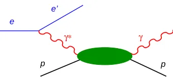
In these processes, the basic mechanism is understood to be a current-curent interaction. In Compton scattering, however, two photons are involved, which means that the information gathered in this reaction is more detailed. In the deeply-virtual variant (DVCS), an incoming electron radiates offa highly virtual photon, that is absorbed by the hadron, which in its turn looses the acquired energy and momentum by radiating off a real photon. The structure of the hadron that plays a role in this reaction is called a generalized parton distribution (GPD) [1], [2]. (For a re-view of GPDs see for instance the paper by Diehl [3].) It can be argued that DVCS is sensitive to the hadronic wave functions obtained in light-front dynamics (LFD).
e
e’
p p
γ∗ γ
Fig. 3.Deeply virtual Compton scattering. DOI:10.1051/epjconf/20100303030
For all these analyses to work, one needs a separa-tion of scales. In DVCS the scales involved are the typical masses of the hadron and the momenta of its constituents, compared to the momenta of the photons. If the latter are much larger that the hadronic scales, factorization can be proved in a number of cases.
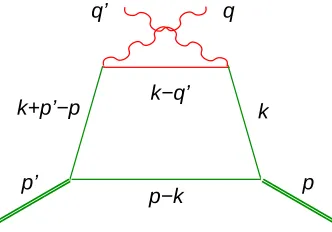
In order to bring out the dependence on the LF wave functions, one studies the contributions of the different am-plitudes that can occur in DVCS. Common lore has it that the handbag diagrams, depicted in Figs. 4 and 5 repre-sent the dominant contributions to the DVCS amplitude. In these diagrams, the hard momenta and the soft momenta are clearly separated.
q’ p
p k+q
k+p’−p
p’
k
p−k
Fig. 4.Direct handbag diagram. The photons and the intermedi-ate quark have high momenta, while the hadron and the quarks directly connected to it have small momenta.
p k
p−k k+p’−p
p’
q’ q
k−q’
Fig. 5.Crossed handbag diagram.
In the cat’s ears diagram, however, this separation does not occur. Therefore, it cannot be expressed in terms of GPD, the quantity that is described by the part of the am-plitude that contains soft hadrons only. As we have shown in a model calculation [4] that the cat’s ears diagram is suppressed, but only at the level of 30%, the extraction of GPDs from DVCS cross sections is not unproblematic.
In this paper we discuss the issue whether the GPDs can be extracted within any reference frame chosen for the description of the reaction and taking the high-Q limit of the propgator of the intermediate quark. This question could come up also in the case of e.g. the determination of a form factor using electron scattering. There a mani-fest covariant calculation shows that the form factor is an invariant quantity. A calculation using the LF approach,
p k
q q’
p’ p−k−q’
k+q
p−k
Fig. 6.Cat’s ears diagram.
see e.g. Ref. [5], reproduces the form factor exactly, if the higher Fock states are included.
In the next section we shall show the connection be-tween LF wave functions and GPDs and see that this for-malism contains elements that raise the suspicion that some treacherous points may be involved.
We shall work in the framework of LFD throughout, because of its well-know advantages:
1. A Fock-space expansion of many-particle states is valid owing to the simplicity of the Fock vacuum. This is re-lated to the spectrum condition on the momentum of any real particle: p+
≥ 0, while for a massive par-ticle p+ must be strictly greater than zero. Therefore, the vacuum, which has p+ =0, cannot create massive particle–anti-particle pairs.
2. In LFD one works with physical degrees of freedom only. No negative-energy particles are included and the LF gauge is free of ghosts.
3. LFD treats physical systems at the amplitude level: LF wave functions are defined independently of the refer-rence frame. They are LF boost invariant.
2 Formalism
In LF dynamics one works with time-ordered amplitudes. The coordinates and momenta are written in terms of LF components, e.g.
xµ=(x+,x⊥,x−), x±= x
0 ±x3 √
2
, x⊥=(x1,x2). (1)
Conventionally, x+is taken as the LF time coordinate, p− the corresponding LF energy. In a Hamiltonian approach the particles are on-mass-shell, while the states are off -energy-shell. In principle, a calculation in LFD should give the same result as a manifestly covariant one if the same physics is incorporated. Problems may arise if approxima-tions are taken that work out differently in different ap-proaches.
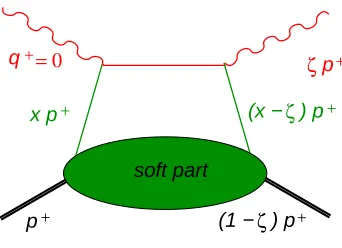
p
p+ (1 − ) pζ +
+
ζ = 0
p−k +
x p (x − ) pζ +
+
q
soft part
Fig. 7.Electron scattering.
definition of the momenta by including the perpendicular and minus momentum components, see Sect. 3, one finds that it is easy to satisfy four-momentum conservation, be-cause q+ =0. Consequently, the condition q2 =−Q2 can be fulfilled for any value of the minus component q−, if
q2
⊥ = −Q2. Another argument in favour of this kinemat-ics is related to the fact that in LF dynamkinemat-ics the vacuum is simplified, because the vacuum cannot fluctuate in mas-sive particle-anti-particle pairs and therefore a photon with vanishing plus-momentum, equal to the plus-momentum of the vacuum, cannot create quark–anti-quark pairs.
An example of the effect of the choice of kinematics is the calculation of the elastic form factor, as illustrated in Fig. 8. If q+ > 0, there are two contributions to the form factor, one that can be described in terms of the lowest Fock-space component of the wave function of the probed hadron, the valence wave function, while the other one in-volves a higher Fock-space component, the non-valence one. It is well known that the limit q+ →0 of the valence part of the form factor may differ from the correct value in some cases, see Ref. [5], the difference being a zero mode.
q
q
p’ p p’ p
ψv ψv ψv ψnv
Fig. 8.Electron scattering. Left: valence part, right: non-valence part.
So we notice that the choice of kinematics amounts to a filter. The upper part of Fig. 7, containing the hard-scattering amplitude, determines which quark structure can be seen.
The connection between the DVCS amplitude and the GPD is given by [3]
M↑↑=M↓↓=−e2q
Z
dx 1
x−ζ+iǫ +
1 x−iǫ
!
H(ζ,x,t),
(2) where the arrows denote the helicities of the photons and H is the GPD. Note that conventionally the GPD is con-nected to the diagonal spin matrix elements only. Eq. (2) is
supposed to be valid in the DVCS limit Q→ ∞, therefore we concentrate here on the hard-scattering part, which is just tree-level Compton scattering.
3 Tree-level DVCS
In Figs. 9 and 10 we show the two hadron diagrams we shall discuss: s channel and u-channel scattering, respec-tively. (We do not include the lepton parts in these figures.)
q’ = p + ζ +
k = x p+ +
+
+ +
k + q = x p
ζ
+ +
k’ = (x − ) p
q = 0+
Fig. 9.s-channel Compton scattering.
q’ = p
+ζ
+k = x p
+ +k’ = (x − ) p
+ζ
+q = 0
++
+ +
ζ
k − q’ = (x − ) p
Fig. 10.u-channel Compton scattering.
The complete amplitude is given by
M=X
h
L({λ′, λ}h)1
q2H({s′,s}{h′,h}), (3)
whereLis the leptonic part of the amplitude andH is the hadronic part, given by:
H({s′,s}{h′,h})=¯u(k′; s′)ǫ∗/(q′; h′)(Os+Ou)ǫ/(q; h)u(k; s) (4) with
Os+Ou= k
/+q/+m (k+q)2−m2 +
k
/−q/′+m
(k−q′)2−m2. (5) The quantities h, h′, s, and s′are the helicities of the pho-tons and hadrons, respectively. The quantitiesλandλ′are the helicites of the leptons in the initial and final states, re-spectively. We take for the hadron (quark) a spin-1/2 field; the photon is of course the usual spin-1 field. We shall work in the LF gauge, viz A+=0.
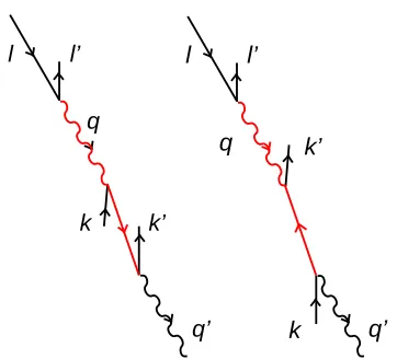
q’
k’
q
l
l’
k
q’
l
l’
k
q
k’
Fig. 11. Kinematics. The leptons are denoted by l and l′, the
hadrons by k and k′, and the photons by q and q′. i Left: s-channel,
right: u-channel.
components: q1=
O(Q), q−=O(Q2).
kµ= xp+,0,0, m
2
2xp2
! ,
qµ= 0,Q,0, Q
2
2ζp+ +
ζm2 2(1−ζ)p+
! ,
k′µ= (x−ζ)p+,0,0, m
2
2(x−ζ)p+
! ,
q′µ= ζp+,Q,0, Q
2
2ζp+
!
, (6)
The momenta are written in the format (p+,p1,p2,p−). The z-components are obtained from the indentity p3 = (p++p−)/√2. Clearly, both photons are moving almost parallel to the z-axis for large values of Q.
In this kinematics we indeed find in the limit Q→ ∞ the form of the denominators occurring in Eq. (2):
Os|Red = lim Q→∞Os=
γ+
2p+ 1 x−ζ,
Ou|Red = lim Q→∞Ou=
γ+ 2p+
1
x. (7)
The polarization vectors of the photons are obtained from the polarization of a photon aligned with the z-axis by a LF boost. The general form for a particle with mo-mentum qµis [7]
ǫ(q;+1)= √1
2 0,−1,−i,− qx+iqy
q+
! ,
ǫ(q; 0)= p1
q2 q +,q
x,qy,
q2 ⊥−q2
2q+
! ,
ǫ(q;−1)= √1
2 0,1,−i, qx−iqy
q+
!
. (8)
For the real photon, we do not need the longitudinal po-larization, but for the virtual one we do. We see that the polarization vectors are singular, which prevents a straight-forward calculation of the amplitudes in this kinematics. In
Table 1.Leiptonic partLof the matrix element.
{λ′, λ} h L({λ′, λ}h)
{+1 2,+
1
2} +1 −Q
1− δ
2ζ+
2ζ δ
{+1 2,+
1
2} 0 −i2 √
2Qζδ
{+1 2,+
1
2} −1 −Q
1−3δ ζ −
2ζ δ
order to obtain meaningful results, we write q+=δp+and make some other changes for consistency. This gives the following momentum for the virtual photon
qµδ= δp+,Q,0, Q
2
2(ζ+δ)p+ +
ζm2 2x(x−ζ)p+
!
, (9)
which has lenght-squared
q2δ=− ζ ζ+δQ
2+δ ζm 2
x(x−ζ). (10) The polarization vectors are
ǫµδ(q;+)= 0,−
1 √
2,− i √
2,− Q √
2δp+
.
ǫµδ(q; 0)= 1 q
q2δ
δp
+
,Q,0,−Q
2 −q2δ √
2δp+
.
ǫµδ(q;−)= 0,
1 √ 2
,−√i
2
, √Q
2δp+
. (11)
Clearly, qµδ=qµ+
O(δ), so all nonsingular quantities reduce to the corresponding ones for δ = 0, the only exception being the polarization vectors. Now we can for any finite value ofδperform the calculation of the matrix elements and obtain finite results.
As we are interested in the DVCS limit, we expand all matrix elements in powers of Q and also in powers ofδ, because in the end we want to take the limitδ → 0. If it exists, the singular kinematics is consistent.
4 Results
In order to be able to calculate the complete amplitude, leptonic and hadronic part included, we need to specify the leptonic kinematics. Ensuring that the transferred momen-tum is qµδwe take
ℓµ= ℓ+,Q,0, Q
2
2ℓ+
!
, ℓ′µ=ℓµ−qµδ, (12)
which are finite forδ→0.
Now we can calculate all matrix elements and expand them in powers ofδ. We shall show some typical results. As we take the leptons massless, the leptonic matrix ele-ments are diagonal in the helicities.
Table 2.Hadronic partHof the matrix element.
{h′,h} {s′,s} H({h′,h}{s′,s})
Full H({h′,h}{s′,s})Red {1,+1} {1
2, 1 2} 2
q
x x−ζ
1+ζ
δ
2
q
x−ζ
x
{1,−1} {1 2,
1 2} −2
q
x−ζ
x
ζ
δ 0
{1, 0} {1 2,
1 2} i
√
2q x x−ζ
1+2ζ
δ − δ
4ζ
i√2
q
x−ζ
x
1+ δ
2ζ
Table 3.Complete matrix element.
{λ′, λ} {h′,h} {s′,s} L1 q2HFull {1
2, 1
2} {1,1} { 1 2, 1 2} 1 Q q x x−ζ
−4δζ22− 6ζ δ − 3 2+ δ 4ζ {1 2, 1
2} {1,0} { 1 2, 1 2} 1 Q q x x−ζ
8ζ2
δ2 + 4ζ
δ −1+ δ 2ζ {1 2, 1
2} {1,−1} { 1 2, 1 2} 1 Q q x x−ζ
−4δζ22+ 2ζ δ − 3 2+ 5δ 4ζ P
h Q1
q
x x−ζ
−4+2δ ζ
{λ′, λ} {h′,h} {s′,s} L1 q2HRed {1
2, 1
2} {1,1} { 1 2, 1 2} 2 Q q
x−ζ
x
−2δζ−1+ δ 4ζ {1 2, 1
2} {1, 0} { 1 2, 1 2} 2 Q q
x−ζ
x
2ζ δ +1−
δ 4ζ {1 2, 1
2} {1,−1} { 1 2,
1 2} 0
P
h 0
Next, we calculate the hadronic part. Again, these ma-trix elements, shown in Table 2, are singular. Finally, we calculate the complete amplitude by performing the con-volution of the leptonic and hadronic parts. We may do so using either the exact propagatorsOsandOuor the reduced ones given by Eq. (7). The results are given in Table 3. We see that after summing the complete amplitude over the virtual photon polarization, the singular parts cancel, but if the reduced hadronic amplitude is used, the complete am-plitude is wrong. Let us emphasize that the contribution of the virtual photon with longitudinal polarization is es-sential for the cancellation, both in the case where the full propagators are used and for the reduced ones.
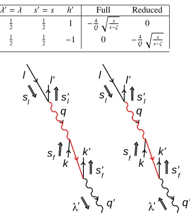
Another feature of the reduced matrix element in this kinematics is the non-conservation of angular momentum. This means that some amplitudes which are forbidden by angular momentum conservation do not vanish if the re-duced hadronic amplitude is used and vice versa. This is illustrated in Table 4 and Fig. 12 for the case where the to-tal incoming spin is 0. If the spins of the fermions in the final state couple to 1, then the photon spin must be op-posite. If one would include in the reduced operators the perpendicular parts of the momenta q and q′, as is done by Radyushkin [8], the violation of angular-momentum con-servation can be expected to be absent. This expectation is based on the results of Carlson and Ji [9], who show that a transverse LF boost, which combines a pure boost with rotations, can flip the spin.
Table 4. Complete matrix element: angular-momentum non-conservation.
λ′=λ s′=s h′ Full Reduced
1 2
1
2 1 −
4 Q
q
x
x−ζ 0
1 2
1
2 −1 0 −
4 Q
q
x x−ζ
q’
q
k’
l’
l
k
s’
q’
q
k’
l’
l
k
s’
s
λ
λ
s
l l f f fs
s
f’
’
s’
l ls’
Fig. 12.Kinematics. The spins are denoted by fat arrows. Left: allowed, right: forbidden.
5 Summary and conclusions
Generalized parton distributions may reveal hadron struc-ture beyond what is known from elastic and deep-inelastic lepton scattering offhadrons. In order to realize its poten-tial one must perform the scattering experiment in such a kinematical setting that the hard momenta are limited to part of the scattering process. The GPD, describing the soft part, must be facorized in the limit of the hard-momentum scale Q→ ∞from the hard-scattering part.
This factorization leads naturally to the idea that the hard-scattering part works like a filter. In DIS and elastic lepton scattering this filter is just the coupling of one pho-ton, while in Compton scattering it involves two photons.
Using a convenient kinematics, we found that the po-larization vectors obtained in light-front dynamics are sin-gular. This problem can be overcome using a near-singular kinematics, which coincides with the convenient one in the limitδ→0,δbeing a small parameter. In order to make the calculations as transparent as possible, we chose to limit our study to the hard-scattering filter. This enables us to obtain analytic results in an exact calculation, not involv-ing any model assumptions about the soft part.
Proceeding with the calculations in the adopted kine-matics, we find that all matrix elements inherit the singu-larity 1/q+(1/δ) of the polarization vectors of the virtual photon. Moreover, the conventional wisdom that the con-tribution of the photon with longitudinal polarization may be neglected owing to the factor 1/pq2occurring inǫ(0) (see Eq. (8)), seems mistaken, as we found this contribu-tion essential for obtaining a finite result.
reason for the violation. Rather, the neglect of the perpen-dicular components must be blamed.
This leads us to our final conclusion: The extraction of GPDs from experimental data may be more subtle than thought before, because an operator reduction as used here, may produce wrong results. So a naive power-counting ar-gument must be considered inadequate.
References
1. X. Ji, Phys. Rev. Lett.78(1997) 610.
2. A.V. Radyushkin, Phys. Lett.380(1996) 417. 3. M. Diehl, Phys. Rept.388(2003) 41.
4. B.L.G. Bakker and C.-R. Ji, Proceedings of Light-Cone’09, Relativistic Hadronic and Particle Physics, Sao Jose Dos Campos, Brazil, 8 - 13 July 2009. Nucl. Phys. B596(2001), 99.
5. J.P.B.C. de Melo, J.H.O. de Sales, T. Frederico, and P.U. Sauer, Nucl. Phys. A631, 574 (1998);
B.L.G. Bakker and C.-R. Ji, Phys. Rev. D62, 074014 (2000).
6. S.J. Brodsky, M. Diehl, and D.-S. Hwang, Nucl. Phys. B596(2001), 99.
7. B.L.G. Bakker and C.-R. Ji, Phys. Rev. D65, 073002 (2002).
8. A.V. Radyushkin, Phys. Rev. D56(1997) 5524. 9. C. Carlson and C.-R. JI, Phys. Rev. D 67. 116002