Perception and reconstruction of two-dimensional,
simulated ego-motion trajectories from optic flow.
R.J.V. Bertin
†, I. Israël
†, M. Lappe
‡Abstract
A veridical percept of ego-motion is normally derived from a combination of visual, vestibular, and proprioceptive signals. In a previous study, blindfolded subjects could accurately perceive passively travelled straight or curved trajectories provided that the orientation of the head remained constant along the trajectory. When they were turned (whole-body, head-fixed) relative to the trajectory, errors occurred. We ask here whether vision allows for better path perception in similar tasks, to correct or complement vestibular perception. Seated, stationary subjects wore a head mounted display showing optic flow stimuli which simulated linear or curvilinear 2D trajectories over a horizontal ground plane. The observer's orientation was either fixed in space, fixed relative to the path, or changed relative to both. After presentation, subjects reproduced the perceived movement with a model vehicle, of which position and orientation were recorded. They tended to correctly perceive ego-rotation (yaw), but they perceived orientation as fixed relative to trajectory or (unlike in the vestibular study) to space. This caused trajectory misperception when body rotation was wrongly attributed to a rotation of the path. Visual perception was very similar to vestibular perception.
Key words: path perception, ego-motion; optic flow; linear heading, circular heading, vision; vestibu-lar.
This paper is a revised edition of Vision Research 2000 vol. 40 #21, pp. 2951-2971
© 2000,2002 R.J.V. Bertin
1— Introduction
Vision provides a wealth of information about our whereabouts in the external world. Much of the infor-mation concerning position and (ego)movement can be gleaned from the optic flow (Gibson, 1950; Gordon, 1965; Koenderink & van Doorn, 1977,1987; Koenderink, 1986; Lee, 1974,1980), the distribution of local velocities over the visual field arising when we move through the world. It has been shown that this information is used throughout much of the animal kingdom. Vertebrates (birds and mammals including humans) use optic flow information in many tasks involving ego-motion (Lee & Young, 1985; Judge, 1990; Lee, 1991; Barinaga, 1991; Lee et al., 1993; Wang & Frost, 1992; Wylie et al., 1998; Lappe & Bremmer, 1999a; Lappe et al., 1999b). But also arthro-pods, especially insects rely on it in many and often re-markably similar ways (Wehner & Lanfranconi, 1981;(Wehner & Lanfranconi, 1981) Götz, 1975; Krapp & Hengstenberg, 1996), notably ants and bees for estimat-ing travelled distance (Collett, 1996; Schöne, 1996).
There is a substantial body of literature providing
psy-chophysical evidence which shows that humans can ac-curately determine their heading direction of linear ego-motion from short optic flow presentations (Warren et al., 1988; Warren, Blackwell et al., 1991; Crowell & Banks, 1993; Royden et al., 1992,1996; van den Berg, 1992,1996; van den Berg & Brenner, 1994a,b; Warren & Saunders, 1995 Banks et al., 1996; Grigo & Lappe, 1999; Lappe et al., 1999a; ). They can also detect their heading direction on circular trajectories (Rieger, 1983; Turano & Wang, 1994; Stone & Perrone, 1997; Warren, Blackwell et al., 1991; Warren, Mestre et al., 1991(Rieger, 1983; Turano & Wang, 1994; Stone & Perrone, 1997; Warren et al., 1991; Warren et al., 1991)). In some cases, additional visual or even non-visual information is required if the simulated movement is to be perceived correctly: this is the case when the optic flow is ambiguous. For example, the flow that results from a linear translation concurrent with a horizontal eye or head or whole-body rotation resembles very closely the flow that results from a tangential, cur-vilinear movement (for short presentations and/or small rotations). In absence of disambiguating extra informa-tion, such a flow may give rise to a perception of travel-ling along a curved path (Banks et al., 1996; Crowell,
! "#$ %% &&' %(' )*+ #, - ./0 0.! 11 2 # - ./0 0.!
3 4 5 0 6 0 , )0 78 9 : 04 && ( 04 ; 4 <
- 0 , .0 70 7, 04 .
1997; Cutting et al., 1997; Royden, 1994; Royden et al., 1992,1994; van den Berg, 1996; Warren & Hannon, 1990; Warren, Blackwell et al., 1991).
Vision is not the only source of ego-motion informa-tion we have. Efference copies provide informainforma-tion about intended movements. Proprioception and inertial information coming from the somatosensory and vesti-bular systems inform about movements actually being made. Combinations of information from these sources can indeed disambiguate the optic flow given as an ex-ample above. When making the appropriate eye move-ments, or when moving the head relative to the trunk in the appropriate way, observers correctly perceive to be moving along a straight path (Royden et al., 1994; Crow-ell et al., 1998). Finally, in absence of visual information, the vestibular (and somatosensory) system can be relied upon to estimate movement, as long as velocity is not constant (Telford et al., 1995).
Recent work from our group (Ivanenko et al., 1997a,b) showed that subjects can perceive aspects of linear and curvilinear movements when displaced blindfolded on a mobile robot, in some cases correctly reproducing (with pen and paper) the perceived travelled trajectory. In ad-dition, they are capable of updating their angular posi-tion relative to a previously seen landmark, even in the absence of semicircular canal input (i.e. with their orien-tation [yaw] fixed in space). They do not, however, seem to use this information about their orientation to im-prove their perception of the trajectory.
In the present paper, we study whether subjects can perform the same task based on visual input, in our case optic flow, alone. That is, we address the question whether human observers can correctly perceive visu-ally simulated, passive ego-movement along 2D trajecto-ries. The visual literature cited above show that humans are capable of instantaneous perception of heading from short optic flow stimuli. The problem we will study here is whether they can also integrate successive instantane-ous heading perceptions to form a coherent percept (re-construction) of the travelled path1? Virtual reality was used to simulate movement of the subjects, after which they were asked to reproduce the movement they had perceived. To this end they could manipulate a model vehicle of which position and orientation were recorded. Several simulated 2D movements were presented; linear and semicircular trajectories, with the observer's orienta-tion fixed relative to either the trajectory, to the external world, to both or to neither. We compare the results with those obtained in the vestibular study (op. cit.).
2— Methods
2.1- Experimental set-up.
Optic flow stimuli were generated on a Silicon Graph-ics Indigo2
/Extreme workstation using the Performer 2.1 libraries, and displayed in a Virtual Research VR4 head
4 <
4 ! = 0 9 =
>
mounted display (HMD; FOV 48° horizontal × 36° verti-cal, 742x230 pixels, 60Hz refresh) worn by the subject. Both eyes saw the same, monochrome, image. The im-age represented a virtual observer's view through the helmet on a dark (black) environment with white dots (4800; homogeneous, random distribution) on a sur-face (50x50m; visible up to 15m ahead) 1m below eye-level (see figure 1a). Optic flow was created by simulat-ing movements of the observer through the virtual envi-ronment, of which between 150 and 200 points were visible at any given moment. Each stimulus consisted of a 2s stationary period followed by 8s of simulated move-ment followed by another 2s stationary period.
Subjects were required to reproduce their perception of the simulated movement after stimulus presentation. Their responses were digitised online by means of a Cal-Comp DrawingSlate II tablet (9"x6": resolution 22860x15240 pixels) that they held on their knees. They manipulated a custom-made input device, containing the coil, switches, circuit board and batteries that were removed from the stylus that came with the tablet. The device's instantaneous position (X,Y) and orientation ( o; resolution approx. 4°) were read from the tablet using custom-written software running on the Indigo, and saved to disk. During the reproduction, a cursor was presented in the VR helmet, showing the device's cur-rent position and orientation, and a trace showing its trajectory. Horizontal and vertical lines intersecting in the centre of the image were also shown as a frame of reference (inset in figure 1a). Buttons on the device al-lowed the subjects to erase unsatisfactory reproductions and accept (save) only those that best represented their percept. Subjects were instructed to remove the device from the tablet during stimulus presentation. A post-hoc compensation was made for the slight difference in as-pect ratio between the VR helmet and the tablet.
2.2- Experimental procedure.
Subjects were seated on a standard office chair. The experimenter gave a brief introduction to the experi-ment, stating that the images they were to see would give the impression of being moved passively, for in-stance on a chair on wheels that can turn around its ver-tical axis. A few possible movements not used in the ex-periment were demonstrated (with the chair) to familiar-ise the subjects with the fact that yaw need not be yoked to the path. The input device was presented to the sub-jects as a vehicle capable of this kind of movements, e.g. a boat or hovercraft (or a helicopter restrained to hori-zontal movement); it will be referred to hereafter as the vehicle. Subjects were allowed to get comfortable with the vehicle and tablet and to train in the reproduction of circular, tangential, movements and rotations in place, both before and after donning the helmet. This also al-lowed to check if and to what extent they had grasped the idea of reproducing movements (2D, 3 degrees of freedom) with the vehicle.
were instructed to concentrate on reproducing the perceived movement's spatial geometry, and to make optimal use of the tablet's surface (resolution optimisation). After validating their response, they could ask for re-presentations of the same stimulus, until they were entirely satisfied with their reproduction. To
minimise response errors due to either memory or drawing artefacts, subjects were asked whether they required a re-presentation when they seemed unsure about their perception. Similarly, when drawing/reproduction problems were noticed, subjects were asked to assess their result (via the image in the
Figure 1. (a) Optic flow impression. The figure shows the first moments of the large radius condition semicircle no-turn). In the experimen-tal conditions, only single dots were seen to be moving, with a slightly higher density and otherwise identical geometry and field of view. The upper left inset shows an example of the reproduction feedback the subjects saw in the HMD: here, the input device was guided through a tangential, curvilinear movement. The upper right inset shows an exploded view of the "vehicle", the input device manipulated by the subjects. Vehicle and vehicle drawing © 1998,1999 M. Ehrette. (b) Representation of the different stimuli presented. Each curve repre-sents a trajectory (X,Y), the arrows point in the direction of the orientation ( o). The figure shows only the large conditions, from left to right, top to bottom; (left): linear lateral ( ), linear oblique 30° ( ), linear oblique 120° ( ) and linear oblique 135° ( ); (middle): semicircle
no-turn ( ), semicircle outward ( ; r=90°); the rotation in place ( ), and semicircle inward ( ; r=-90°); (right): semicircle forward ( ; r=0°), semicircle full-turn ( ) and linear half-turn ( ).
-12
-10
-8
-6
-4
-2
0
2
4
6
8
10
-2
0
2
4
6
8
10 12 14 16 18 20 22 24 26 28
Position, Y
Position, X
HMD), and to either erase and redraw it, or view another presentation and redo the reproduction. Experiments generally did not last longer than one hour, depending on the time spent in familiarising with the set-up, and on the number of re-presentations requested.
The simulated movements (figure 1b) were based on the movements presented in Ivanenko et al. (1997b); some were actual simulations thereof. Thus, triangular veloc-ity profiles starting from zero velocveloc-ity were used, both for linear and angular speed. The angular acceleration was always either 11.46°/s2 (0.2rad/s2) or zero. The
fig-ure shows the actual scale (in meters) of the simulated movements. The simulated movements were presented in random order to the subject. Iconic representations (pictograms) will be used throughout to simplify recog-nition; the tables in the appendix only use pictograms.
We will distinguish three orientations: the orientation of the observer in space ( o; independent of the trajec-tory), the orientation of the trajectory ( p: the angle in space of the tangent to the trajectory) and the observer's orientation relative to the trajectory, r = o - p. Simi-larly, we will distinguish two types of rotation (change in orientation): o (yaw) and p (the rotation of the tra-jectory). Angles are expressed in degrees, with positive values indicating clockwise rotation.
The stimuli fall into 3 distinct classes, as listed below:
Stimuli with the observer's orientation (yaw) fixed in space:
I.Linear translation with the observer's orienta-tion oblique at r= o=30° (condition linear oblique 30° ), o=135° (condition linear oblique 135° ) and o=120° (condition lin-ear oblique 120° ). Linear acceleration was 1.18m/s2, average translation speed 2.33m/s.
(In these stimuli, orientation is also fixed rela-tive to the trajectory.)
II.Semicircular trajectory with o=0° (condition semicircle no-turn , condition III in op.cit.). Stimuli with the observer's orientation fixed relative to
the trajectory:
III.Semicircular trajectory with the observer look-ing outward ("centrifugal": r=90°; condition semicircle outward ).
IV.Semicircular trajectory with the observer look-ing inward ("centripetal": r=-90°; condition semicircle inward ).
V.Semicircular trajectory with tangential orien-tation ( r=0°; condition semicircle for-ward ; condition II in op.cit.)). The average speed of rotation ( o) in III, IV and V was -22.5°/s.
Stimuli with the observer's orientation changing in space and relative to the trajectory:
VI.Semicircular counterclockwise trajectory with a full rotation ( o=360°, starting at 0°; condi-tion semicircle full-turn ; condition V in op.cit.)2. The average speed of rotation ( o) was
45°/s.
VII.Linear translation with o=180° starting at 0°, (figure 1d; condition linear half-turn ; con-dition VI in op.cit.).
VIII.A o=-180° clockwise rotation in place ( ; condition I in op.cit. ). The average speed of ro-tation ( o) was -22.5°/s.
The semicircular conditions were all presented with a large (5m) and a small (1.5m) radius. In these conditions, the average speed of translation was 0.59m/s for the small, and 1.96m/s for the large radius, while the direc-tion of transladirec-tion rotated at an average speed of 22.5°/s. Condition linear half-turn was also presented in two lengths: 7.8m and 4.7m. In the short version, simulated acceleration was 0.3m/s2, and the average speed of
trans-lation 0.59m/s. In the long version, acceleration was 0.5m/s2, and the average speed of translation 0.98m/s.
Both had an average speed of rotation ( o) of 22.5°/s. In the vestibular experiment, only the small/short condi-tions were used.
These experimental trials were preceded by 1) a sim-ple forward translation and 2) a lateral translation ( o=90°: condition linear lateral ). For these two stim-uli, the subjects were given feedback to arrive at the cor-rect interpretation of the simulated movements; this served as a final check whether they completely grasped the task, and to help them get used to the optic flow and its presentation in the helmet3.
23 Subjects (aged 20 to 50 approximately) participated in the experiment. All subjects saw the stimuli presented above. Of these, 16 subjects saw an additional set of stimuli (containing landmarks) that will be reported on in a future paper. The other 7 subjects saw a stimulus set designed to test for a possible influence of the stimuli's velocity profiles. To rule out such an effect, all stimuli were presented twice to these subjects: once with the tri-angular velocity profile and once with constant velocity (and with identical duration) — intermingled in random order. To mask the abrupt transition from stationary to movement in the constant velocity stimuli, dots had a limited lifetime during the initial stationary period, in-creasing from 3 frames to approx. 85-100 frames. Where necessary, we will refer to these two sub-populations as Group 1 (with 16 subjects) and Group 2 (with 7 subjects) respectively.
After the experiment subjects were asked for their general impression of the stimuli and of their task. The subjects in Group 2 were also asked if they had re-marked that each movement had been presented in two different ways (that is, with a triangular and a constant velocity profile).
2.3- Data analysis.
Some subjects showed better manual skills at
!"
# $ % & '
# (
lating the vehicle than others, and thus the responses cannot directly be compared amongst each other or to the stimuli. The traces were therefore filtered to remove clutter from the initial positioning of the vehicle and jerk movements due to (transient) individual problems with the vehicle's handling. Such artefacts are easy to recog-nise and include: 1) samples with the device resting in the same location and orientation for prolonged periods, 2) clutter resulting from putting the vehicle in the de-sired starting position and/or orientation and 3) abrupt movements caused by lifting the vehicle to validate a re-production. These are all easily identifiable by compar-ing response plots (cf. figures 1 and 2) with side-by-side X, Y and o time-series; 1) as leading or trailing horizon-tal lines on the time-series, 2) as random variations in X and Y with o approaching the intended value (up to the moment when X and Y start changing systematically and smoothly) and 3) as a sharp jump in X and/or Y, in extreme cases followed by a return to the desired posi-tion4.
After filtering, the data were resampled to 20 equidis-tant points per trace. This was done with an interpolat-ing algorithm usinterpolat-ing cubic splines. Individual splines were fitted to the Xi, Yi and oi co-ordinates, using Li —
the length of a trace from its beginning (i.e. the travelled distance) up to (Xi,Yi) — as the independent variable;
where i is the sample/point number (i=1…n).
Resam-" ) ' #
#
# # * +$ ( #
# #
pling was then achieved by taking the "splined" Xj, Yj and
oj at 20 points L*j, with L* linear and between L*1 = L1 = 0 and L*20 = Ln.
Our protocol does not allow us to analyse reproduced speeds, nor scale. We thus focus our quantitative analy-ses on orientation ( ) and change in orientation (rota-tion; ) only. The three orientations and the two types of rotation that we can distinguish have been introduced above. Of these, we use the following observables as in-dices to quantify or results: p, o and the average ori-entation relative to the path < r>; cf. figure 1c. p is computed as the average difference between two con-secutive tangent measures, times the number of seg-ments in the curve. Its value is zero for a straight line, or 180° for a semicircular trajectory. Its standard deviation measures the constancy of path rotation. The standard deviation is 0 for e.g. a perfectly straight line or for a perfect semicircle. The perceived yaw o is calculated by summing the o values in the resampled points, minus the initial orientation (such that for 2 observer turns, o=720°). Finally, < r> is computed as the average of the difference between orientation and heading (orienta-tion minus heading, where heading is the tangent to the reproduced path). This measure gives 0 for a correct re-production of a tangential movement, and a zero stan-dard deviation for an orientation remaining perfectly fixed relative to the trajectory. For this index, p, o and their difference are all expressed as values between [-180°,180°].
3— Results
3.1- General observations.
Integration of instantaneous self-motion information from optic flow proves to be possible — at least to a cer-tain degree — but it is cercer-tainly not always an easy task. In fact, subjects found the task quite difficult, but did not experience discomfort caused by the stimuli. Most sub-jects indicated that they had experienced the impression of ego-motion, but that this impression had not been equally strong in all conditions.
Several different "strategies" for reproducing the movement were observed. For instance, some subjects made reproducing movements with the vehicle during the stimulus presentation. A few subjects asked for a large number of re-presentations to verify a representa-tion of the path they had perceived. Most subjects, how-ever, did not ask for more than 2 presentations, and were satisfied with a single presentation for most of the stimuli. Their perception mostly did not differ very much between presentations of the same stimulus. They did however forget the direction of (especially) o rather frequently, and corrected this in a 2nd presentation.
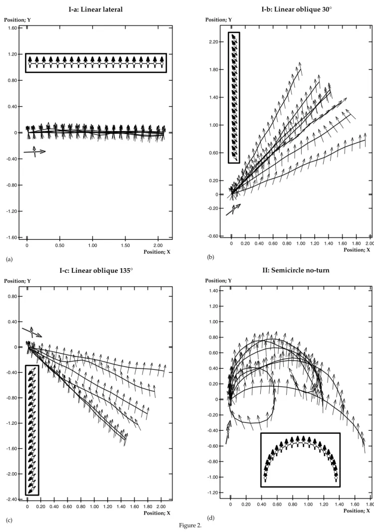
Figure 2 (panels a through j) shows a selection of sub-jects' reproductions. It can be seen that the variability among subjects' responses depends on the stimulus. Generally speaking, optic flow fields simulating what are apparently simple movements give rise to correct re-sponses (at least as far as the trajectories' form is con-cerned), with little variation between subjects. Such is Figure 1. (c) Explication of the indices used in the quantitative
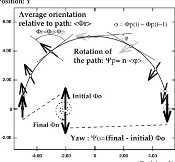
analyses. p, the average rotation of the path is calculated from the average difference between the tangents to the trajectory in 2 consecutive (resampled) points, multiplied by the number of seg-ments per curve (19). The total yaw o is calculated by (non circu-lar) summation over o, minus the initial orientation; thus, 2 full observer turns give o=720°. The average orientation relative to the path, < r>, is calculated as the average difference between o and p in the 20 resampled points. All these measures are ex-pressed in degrees and averaged over subjects. In this example (clockwise semicircle with counterclockwise yaw; not used in the experiments), o=180°, p=-180° and < r>=179.7°±109.8°.
-2.00 0 2.00 4.00 6.00
-4.00 -2.00 0 2.00 4.00
Position: Y
Position: X
Yaw : Ψο=(final - initial) Φo Rotation of
the path: Ψp= n⋅<ϕ> Average orientation
relative to path: <Φr>
Φr=Φo-Φp
ϕ
Initial Φo
Final Φo
ϕ = Φp(i) − Φp(i−1)
Figure 2. (a)
-1.60 -1.20 -0.80 -0.40 0 0.40 0.80 1.20 1.60
0 0.50 1.00 1.50 2.00
Position; Y
Position; X
I-a: Linear lateral
(c)
-2.40 -2.00 -1.60 -1.20 -0.80 -0.40 0 0.40 0.80
0 0.20 0.40 0.60 0.80 1.00 1.20 1.40 1.60 1.80 2.00
Position; Y
Position; X
I-c: Linear oblique 135°
(d)
-1.20 -1.00 -0.80 -0.60 -0.40 -0.20 0 0.20 0.40 0.60 0.80 1.00 1.20 1.40
0 0.20 0.40 0.60 0.80 1.00 1.20 1.40 1.60 1.80
Position; Y
Position; X
II: Semicircle no-turn
(b)
-0.60 -0.20 0 0.20 0.60 1.00 1.40 1.80 2.20
0 0.20 0.40 0.60 0.80 1.00 1.20 1.40 1.60 1.80 2.00
Position; Y
Position; X
I-b: Linear oblique 30°
Figure 2 (continued). (e)
-0.30 -0.10 0 0.100 0.30 0.50 0.70 0.90 1.10 1.30 1.50 1.70 1.90 2.10 2.30
-0.20 0 0.20 0.40 0.60 0.80 1.00 1.20 1.40
Position; Y
Position; X
III: Semicircle outward
(f)
-1.60 -1.20 -0.80 -0.40 0 0.40 0.80 1.20 1.60
-0.50 0 0.50 1.00
Position; Y
Position; X
IV: Semicircle inward
(g)
-0.70 -0.50 -0.30 -0.10 0 0.100 0.30 0.50 0.70 0.90 1.10 1.30 1.50 1.70
0 0.20 0.40 0.60 0.80 1.00 1.20 1.40 1.60
Position; Y
Position; X
V: Semicircle forward
(h)
-1.40 -1.00 -0.60 -0.20 0 0.20 0.60 1.00 1.40 1.80
-0.50 0 0.50 1.00
Position; Y
Position; X
VI: Semicircle full-turn
the case for stimuli in which the simulated speed of translation is high relative to the simulated rotation speed (figure 2a-d). In the case of more complicated movements, subjects increasingly detect (or reproduce) only certain properties of the simulated movement. Quite often subjects report a rotation in place rather than a movement that contains translation.
A remarkable result is that none of the subjects in Group 2 noticed that there were two different velocity profiles. In addition, there is no significant difference in perception of the stimuli with triangular velocity profile, and those with constant velocity. In the following text we will therefore make no distinction between data from conditions with a triangular or constant velocity profile.
Once a stimulus has been associated with a certain movement, ("understood", whether correctly, or not), it is recognised almost all the time.
3.2- Response classification.
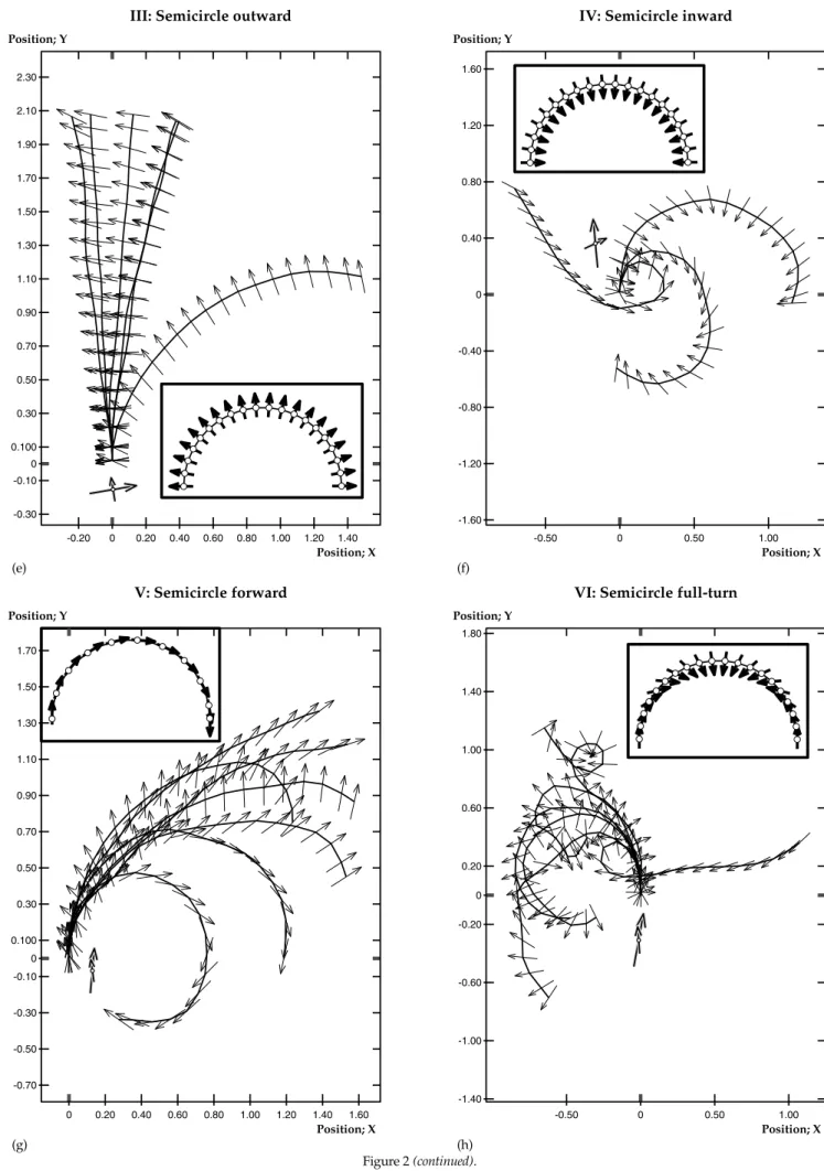
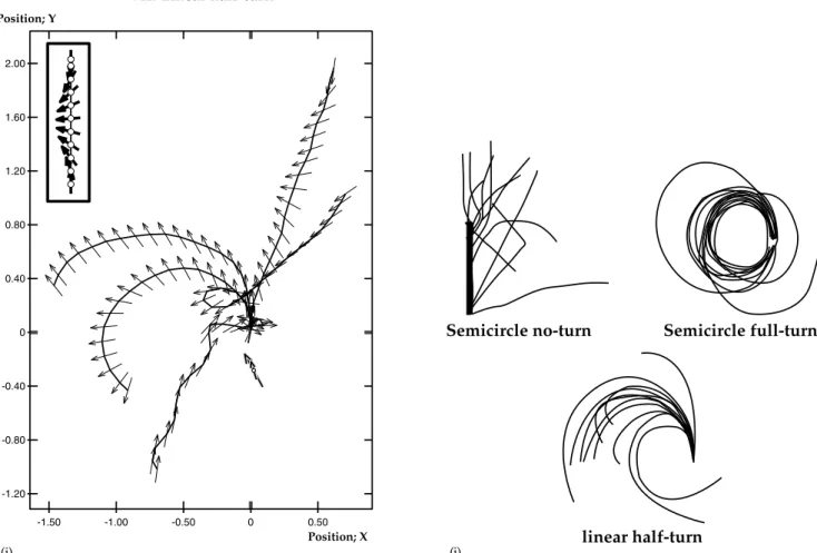
As mentioned above, the degree of correctness of the subjects' responses (performance) varies between condi-tions and subjects. We assess performance qualitatively by scoring globally correct responses, and responses with the correct type of trajectory. A globally correct re-sponse is one that retains the crucial components of the actually presented movement. Thus, for a lateral (oblique) translation, a reproduced movement is glob-ally correct when it is clearly intended to be linear, has the correct direction and the observer's orientation oblique to the path. For a complex movement such as condition semicircle full-turn (a counterclockwise semicircle with o=360°), a globally correct response would be a counterclockwise curvilinear trajectory with the orientation changing in counterclockwise direction relative to the trajectory. The initial observer orientation and the initial direction of movement (e.g. 0°, or 90°, in Figure 2. A selection of reproductions from Group 2 (a-j): all responses to the large/long stimuli with triangular velocity profile. The stim-uli are listed in the figures' titles, which also refer to the stimulus enumeration in the Methods. The responses are filtered and resampled as described in the Methods. To clarify the presentation, the trajectories were then translated to start in the origin and normalised to uniform length, and the responses were rotated as follows. For the conditions with fixed o (in the stimulus; figures 2a through d), the individual re-productions were all rotated over the same angle, such that the resulting orientation averages to 0°. In the other conditions, the reproduc-tions were rotated such that the 1st trajectory segment is oriented at 0°. Finally, the reproducreproduc-tions received additional smoothing. The "clock face" display of two arrows indicates the average initial p (the longer arrow) and the average initial o (the smaller arrow). The insets show the stimulus. The indices for the sets shown in the panels are (all values in degrees): (a) Ia, linear lateral: < r>= 90.52 ± 5.833; p= -3.836 ± 7.634; o= -15.89 ± 8.222; (b) Ib, linear oblique 30°: < r>= 46.52 ± 5.659; p = -1.167 ± 7.498; o = 7.137 ± 17.12; (c) Ic, linear oblique 135°: < r>= 121.4 ± 6.059; p = 3.255 ± 2.950; o = -4.797 ± 7.220; (d) II, semicircle no-turn: < r>= 93.49 ± 61.62; p = -225.0 ± 93.42; o = 1.100 ± 9.242; (e) III, semicircle outward: < r>= 83.98 ± 7.169; p = -23.65 ± 37.63; o = -30.15 ± 15.87; (f) IV, semicircle inward: < r>= -98.40 ± 60.11; p = -294.1 ± 64.57; o = -199.2 ± 70.01; (g) V, semicircle forward: < r>= 31.20 ± 16.12; p = -159.4 ± 75.77; o = -117.2 ± 92.82; (h) VI, semicircle full-turn: < r>= -97.48 ± 50.63; p = 196.8 ± 263.4; o = 158.7 ± 269.7; (i) VII, linear half-turn: < r>= -142.7 ± 72.51; p = 128.3 ± 172.7; o = 115.6 ± 60.17; (j) The trajectory drawings from the vestibular experiment, conditions semicircle no-turn, semicircle
full-turn and linear half-turn. (i)
-1.20 -0.80 -0.40 0 0.40 0.80 1.20 1.60 2.00
-1.50 -1.00 -0.50 0 0.50
Position; Y
Position; X
VII: Linear half-turn
(j)
Semicircle no-turn Semicircle full-turn
space) cannot be derived from our stimuli. Thus, we only consider the initial orientation with respect to the initial orientation of the path, but we disregard the abso-lute, space-relative initial orientation and the initial di-rection of the reproduced movement. In other words, for the condition semicircle outward, a circular path starting at an angle of 0° forward with the observer oriented
ap-proximately perpendicularly outward (say, 80°) is equally correct as a circular path starting at an angle of -40° ("north-eastward") with the observer oriented 40° outward.
Figure 3 shows a classification of our data according to these principles. For completeness, the "raw" data are listed in Table 2, which also lists the number of samples per condition and group. The figure and the table also list a score of responses in which the type of trajectory reproduced was correct, i.e. trajectories that preserve a) the curvilinearity of the stimuli semicircle inward ; semicircle forward ; semicircle no-turn and semi-circle full-turn , or b) the linearity of the stimuli linear lateral , linear oblique , , and linear half-turn . The table also lists the number of rotation in place responses observed.
When the observer's orientation is fixed in space, per-formance is generally good. This is much less the case for the conditions in which the orientation is fixed only relative to the trajectory, or not at all. Two general obser-vations can be made for these stimuli: 1) there are many rotation in place responses; 2) in general, there are more globally correct responses to the large/long stimuli than to the small/short (e.g. the two conditions semicircle
for-ward ).
Some more detailed observations will be made in the presentation of the results below.
3.3- Quantitative analyses.
The results of the quantitative analyses are shown in figures 4 and 5. The detailed results are listed in Table 3. The table also lists the initial heading (the orientation of the trajectory's 1st segment), in addition to the values of
the three indices introduced above, p, o and < r>. All these observables are averaged over subjects, per condition. Average initial orientation is given for the
Figure 4. (a) p for all conditions but the rotation in place. Shaded, striped bars show the expected (i.e. stimulus) values. Asterisks indicate significance of difference with the expected values. Errorbars show standard deviation of the mean. Asterisks indicate significant differ-ences from the expected values, determined by t-tests using mean and average standard deviation; * p< 0.05, ** p< 0.005, *** p< 5·10-4 (Student's t). For the conditions that were shown in two sizes, the response to the large/long stimulus is shown in the left-hand bar, the small in the right-hand bar. There is a significant undershoot for the large semicircle outward: this stimulus is often seen as a lateral transla-tion. It can clearly be seen that a change of orientation relative to trajectory and space is often attributed to a rotation of the path instead
(semi-circle full-turn and linear half-turn ). (b) o for all conditions. The rotation in place condition is shown leftmost. All presentation de-tails as in figure 4a.
(a)
-300°
-200°
-100°
0°
100°
200°
300°
400°
500°
600°
700°
% & ' ( * + , ) - .
Ψp
Condition
Linear stimuli, fixed orientation Curvilinear stimuli, fixed orientation Stimuli with nonfixed orientation Subjects’ responses
** ** *
***
(b)
-300°
-200°
-100°
0°
100°
200°
300°
400°
500°
600°
$ % & ' ( * + , ) - .
Ψo
Condition
Rotation in place stimulus Linear stimuli, fixed orientation Curvilinear stimuli, fixed orientation Stimuli with nonfixed orientation Subjects’ responses
*** ***
***
Figure 3. Performance observations: globally correct responses and responses with the correct type of trajectory, each expressed as a percentage of the number of observations. Percentages shown are calculated over all subjects. The errorbars show the standard deviation in the mean of the per-group performances. Stimulus linear oblique 120° ( ) was not presented to Group 2. Compare with Table 2 in the Appendix, which lists absolute values and numbers of observations. Conditions are labelled with iconified representations of the stimuli. For conditions that were presented in two sizes, the responses to the large/long stimulus are always shown as the leftmost bar, as indicated in the graph. See the text for the remaining details.
100% 80% 60% 40% 20% 0% 20% 40% 60% 80% 100%
$% & ' ( * + , ) - .
Condition
Globally correct responses
Trajectory correct responses
stimuli, and also averaged over all subjects' responses. Only responses that were not rotations in place, and without rotation in the wrong direction are included in the analysis. The number of responses retained is listed in the table. This excludes responses that are clearly un-correlated with the stimulus, but includes the following frequent misinterpretations: 1) lateral translations in con-dition semicircle outward ; 2) more-than-180°-arc (| p| >180°; full circle, spiral, …) trajectories5 with p
and o in the right direction in condition semicircle full-turn and 3) curvilinear trajectories with o in the right direction in condition linear half-turn . < o> is undefined for rotations in place, so for condition we give only the initial heading and the average o (for all responses), and p for responses that are not rotations in place.
Differences between measured responses and the psented (ideal) values, and between per-condition re-sponses are tested with Student's t-tests.
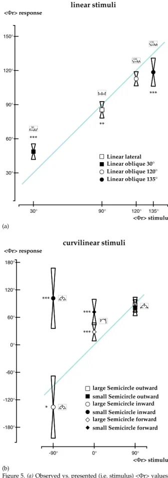
The rotation of the path ( p) and the reported yaw ( o) are shown in figures 4a and 4b respectively (narrow bars with heavy outline), together with the presented val-ues (broader bars with light outline). Both properties gen-erally seem to be well perceived. Figure 5 shows < r>, reported versus presented, for the conditions with fixed
r. Correct responses would fall on the shaded line. A quick glance at these figures would suggest that — albeit considerable variability — the task is on average well performed by our subjects. However, not all re-sponses were included in the computation of the quanti-tative results (compare the N columns in Tables 2 & 3), and we have not yet considered the reported initial heading and orientation. Therefore we will now proceed to a condition-per-condition analysis, referring to the qualitative observations where appropriate.
In the linear lateral condition , responses are near perfect (figure 2a). Subjects maintain almost the correct r (< r> -90°) and they reproduce trajectories which are close to linear on average ( p < 5°). However, since they assume an initial o=0°, their initial heading is ap-proximately 90° to the right. A similar type of response can be observed in the other linear stimuli, conditions lin-ear oblique 30° (figure 2b); 120° and 135° (figure 2c). Here, there is overshoot of the smaller an-gle (approximately 60%; linear oblique 30°) and up to 12% undershoot of the larger angles (linear oblique 120° and 135°). Thus, in these conditions, in which orientation is fixed relative to the trajectory and in space, perceived orientation is approximately correct relative to the trajec-tory, but not in space. As a result, condition linear oblique 30° is perceived as a forward movement, and conditions linear oblique 120° and 135° as backward (initial heading less than 90° rightward and more than 90° rightward respectively). This is not erroneous or inaccu-rate perception; our stimuli do not contain any informa-tion whatsoever about the initial orientainforma-tion.
In the case of condition semicircle no-turn (figure
Figure 5. (a) Observed vs. presented (i.e. stimulus) < r> values, for the 4 linear stimuli with fixed o. Errorbars show average standard deviation (averaged over per-subject values). Correct responses would fall on the grey line. All values in degrees. Asterisks indi-cate levels of significance of difference with presented value: * p< 0.05, ** p< 0.005, *** p< 5·10-4 (Student's t). (b) Observed vs. pre-sented (i.e. stimulus) < r>, for the semicircular conditions with fixed r. Presentation as in figure 5a.
(b)
-180°
-120°
-60°
0°
60°
120°
180°
-90° 0° 90°
<Φr> response
<Φr> stimulus curvilinear stimuli
*
+
+
,
large Semicircle outward small Semicircle outward large Semicircle inward small Semicircle inward large Semicircle forward small Semicircle forward ***
*** ***
* (a)
30°
60°
90°
120°
150°
30° 90° 120° 135°
<Φr> response
<Φr> stimulus linear stimuli
%
&
'
(
Linear lateral Linear oblique 30° Linear oblique 120° Linear oblique 135° ***
***
2d), the quantitative results repeat what was already evident from the qualitative results in figure 3: these stimuli are perceived correctly. The differences from the expected values are all non-significant.
In condition semicircle outward (figure 2e), < r> is perceived correctly, although there is more variability than in the linear conditions. In the stimulus with the large radius, the optic flow resembles much more the laminar flow of a lateral translation than in the small radius stimulus. Indeed approximately half the subjects reproduce linear trajectories. p confirms this: for the large radius, p < 180° (p< 0.001); for the small radius, p is more than 2x larger at p 0.08. This difference also shows in o, which approximates p and is thus too small (significant at p< 10-5 for the large radius),
although less so (larger) for the small radius (p< 0.03). Initial heading is mostly to the right, even for the correct responses.
Condition semicircle inward (figure 2f) is clearly difficult. Most of the subjects who perceive a movement other than a rotation in place see a curvilinear trajectory. There is no consistent perception of ego-orientation ( o or r), but for the small radius version, curvilinear responses typically have either a "centrifugal" r 90°, or, in some cases, o fixed in the environment. The large radius stimulus is perceived as a backwards movement ( < r> > 90°; p< 0.02). There is also a tendency to perceive a trajectory spanning more than half a circle ( p > 180°). o is approximately correct, however.
A large number of the curvilinear trajectories reproduced for condition semicircle forward (figure 2g) maintain a fixed r — only oriented outwards, "centrifugal" (< r> > 0°; almost all for the small radius; almost 50% for the large radius in Group 2). This causes a significant undershoot of o (p< 0.001). Perception is better for the stimulus with the large radius (figure 3). Indeed, < r> is smaller (p< 10-6) and the initial heading
is on average more forward (p< 0.002) for the large than for the small radius. Also, a larger number of curvilinear trajectories are perceived in the large radius condition (figure 3).
Subjects have the greatest problems with the conditions in which orientation is not fixed at all; semicircle full-turn (figure 2h) and linear half-turn (figure 2i). The reported < r> is actually negative instead of 90°. In addition, p is too large; between 50% and 150% in condition semicircle full-turn (p< 0.02; p< 0.0001 in linear half-turn). o is more or less
correct, though6. This combination of approximately the right amount of yaw combined with a too curved trajectory explains the negative < r> values: o "trails" relative to p (see figures 2h and 2i). In condition linear half-turn , p is on average closer to the amount of simulated o than to the actually simulated p = 0°. This hints at what probably happens: subjects seem to attribute o to p. This also explains the overshoot of the p in condition semicircle full-turn .
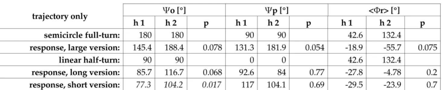
Our results thus suggest that subjects assume that the rotation they perceive is due to a rotation of their trajectory, at least for a large part. Do they at some point notice the difference between stimulus and perception that will inevitably be caused by this illusion, or do they stick to their initial perception? To test this, we calculated our measures independently for the two halves of each response, and tested for differences using analyses of variance (subjects x conditions x halves). When tested over all conditions, there was no significant difference between the first (h1) and the second (h2) half of the responses, in neither of the 3 measures. There are differences however for the large semicircle full-turn, and the long and short linear half-turn: see Table 1.
Subjects report significantly more yaw in the second half of their response than in the first ( o main effect: F(1,12)=6.33, p< 0.027). In condition semicircle full-turn, the reported trajectory is also more curved in the second half ( p), whereas the larger value for < r> would sug-gest that the subjects do indeed perceive that their orien-tation changes relative to the trajectory.
4— Discussion
We studied the perception of ego-movement during visually simulated passive 2D displacements in the hori-zontal plane. The displacements simulated straight or curved trajectories, with in some cases ego-rotation rela-tive to the trajectory and/or in space. Specifically, we asked whether human observers can perceive (recon-struct) such displacements from long (8s) optic flow presentations. It is well documented that humans can perceive instantaneous heading from short optic flow presentations (generally less than 1s); perception of our longer simulated movements could e.g. be based on in-tegration of the instantaneous perception of heading. We investigated the subjects' reproductions of their
percep-trajectory only o [°] p [°] < r> [°]
h 1 h 2 p h 1 h 2 p h 1 h 2 p
semicircle full-turn: 180 180 90 90 42.6 132.4
response, large version: 145.4 188.4 0.078 131.3 181.9 0.054 -18.9 -55.7 0.075
linear half-turn: 90 90 0 0 42.6 132.4
response, long version: 85.7 116.7 0.068 92.6 84 0.77 -27.8 -4.78 0.2
response, short version: 77.3 104.2 0.017 117 104.1 0.69 -29.5 -23.9 0.7
Table 1.The three quantitative measures calculated for the first (h1) and second (h2) halves of the conditions with orientation changing relative to space and to the trajectory, presented and subjects' responses. The p values indicate the significance of the difference between the first and second halves of the subjects' responses. The small condition semicircle full-turn is excluded because of an insufficient number of observations.
tion of both orientation (ego-rotation, yaw), and dis-placement (trajectory). We compared the results with an earlier study addressing vestibular perception of identi-cal, physical displacements in blindfolded subjects.
Our results show that under certain restraints that de-pend on the stimulus, the type of displacement can be perceived; directions, the form of trajectory ( p) and the average orientation relative to the trajectory (< r>). As the optic flow does not provide information on absolute linear ego-motion speed, an absolute judgement of the travelled distance cannot be made. This is also the case for the vestibular system where the double integration of the otolith-provided acceleration signal does not yield a correct measure of distance travelled (Glasauer & Israël, 1993; Israël et al., 1993): subjects do not correctly estimate the length of linear trajectories travelled passively. But human observers are quite capable to make relative based distance judgements from optic flow (Bremmer & Lappe, 1999; Bremmer et al., 1999).
4.1- Perception of trajectory.
Generally speaking, trajectories were correctly per-ceived when the simulated movement contained rela-tively little rotation, or none at all. Thus, perception of the trajectories with the observers' orientation ( o) fixed in space was good. For the linear trajectories, < r> was overshot at 30°, while for 120° and 135° it was under-shot. This range effect (a common phenomenon, e.g. also observed for angular perception in vestibular studies) is possibly due to errors in the estimation of the vehicle's orientation and/or the drawn trajectory. On the one hand, it has been shown that humans can detect their heading direction with an accuracy of up to 1° although they generally underestimate (verbal report: Cutting, 1986; discrimination: Warren et al., 1988; Warren, Black-well et al., 1991). But on the other hand, nominal ("sloppy") heading direction judgements might be more useful in everyday life than exact judgements (Cutting et al., 1997)).
The curvilinear trajectories with orientation fixed rela-tive to the trajectory, could also be perceived correctly. In general, perception was better for the larger radius. When the radius was smaller, the simulated movements contained relatively more rotation. As a result, almost half the subjects reported rotations in place. However, the remainder of the subjects perceived curvilinear
tra-jectories, of too high curvature.
Thus, in most of the cases discussed above, subjects perceived a curvilinear trajectory when the stimulus was curvilinear, if they perceived a trajectory at all. Often, they also reported a semicircular trajectory. Theoretically, they can detect this from the optic flow because the simulated angular velocity is specified unambiguously. Observation of the subjects during the experiment, and the impressions recorded after the experiment suggest another explanation: trajectories were often judged as more than a quarter arc, but less than a 3/4 or full circle, thus a semicircle was assumed. Subjects applied the same categorisation in vestibular tests, and probably also in the judgement of yaw that will be discussed next.
4.2- Perception of orientation.
The optic flow provides absolute angular velocity in-formation, in contradistinction to the information about linear velocity. Humans can use this information to ex-trapolate a tangential, curvilinear trajectory in order to determine whether they will pass to the left or to the right of a target shown after a stimulus (heading detec-tion on curvilinear trajectories, see e.g. Warren, Mestre et al., 1991; Stone et al., 1997). In our experiment, we also find that in most cases subjects report total amounts of yaw that are not significantly different from the actual values. Again one could argue that this overall good performance is due to the subjects' assumption that we presented only "cardinal" amounts of rotation (0°, 180° and 360°), such that "too large for 90°" leads to "180°". Large simulated translation speeds can interfere with the correct perception of rotation, though. Such is the case for the large radius outward- and forward-looking movements in which subjects undershot their rotation significantly.
It happens more often, however, that changes in orien-tation disturb the perception of translation. To such an extent that subjects often lose a coherent perception of translation when the orientation changes in space or in space and with respect to the trajectory, and perceive a rotation in place instead.
The effect of large rotation on the perception of trans-lation is clearest in the cases in which the orientation changes with respect to both the world and the trajec-tory. We presented two such cases, one a semicircle with a full, 360° rotation of the observer, and the other a
lin-Table 2. Summary of results. Results are based on the last response given for each condition (in case the subject asked re-presentations). Per condition, the number of globally correct responses, trajectory correct responses (trajectory only) and, where applicable, the number of ro-tations in place is reported for the 2 groups. Globally correct responses are those which contain a certain minimal set of properties of the correct response: form and direction/orientation of trajectory (thus, these responses are a subset of the trajectory correct responses); type and direction of [change in] orientation. Further specifications are given in the table, per condition. The initial orientation and heading are always disregarded. The total number of responses per group is given in the N column. For Group 2, columns are divided in two equal halves, with the left halve listing the observables for the triangular-velocity condition, and the right halve for the constant-velocity condi-tion. Cw indicates clockwise rotation, CCw counterclockwise rotacondi-tion.
Condition semicircle outward : In Group 1, there were 7 linear lateral translations reported for the large stimulus, and 1 for the small. In Group 2, these figures were 5; 3 for the large condition (triangular vs. constant velocity profile), and 2; 0 for the small.
Condition semicircle no-turn : one subject in Group 2 systematically reports a full circular movement with constant (space-fixed) orien-tation.
Condition linear half-turn : the linear trajectories reported are all — but 2 — correct responses. In this condition, globally correct re-sponses are not necessarily also trajectory correct rere-sponses!
Condition rotation in place : the "trajectory only" column lists the number of responses consisting of curvilinear or linear trajectories with the orientation orthogonal to the path; there is thus no overlap with the globally correct responses!
condition globally correct = trajectory only rotations in place N
Cw rotation in place (curvi)linear
orthogonal
Gr. 1 15 0
Gr. 2 2 3 4 3
N/A 16
7
rightward linear, lateral r linear
Gr. 1 15 15
Gr. 2 6 7 6 7
no RIPs 16
7
rightward linear, oblique r linear
Gr. 1 11 15
Gr. 2 5 6 7 7
no RIPs 16
7
rightward linear, oblique r linear no RIPs
Gr. 1 8 14 16
rightward linear, oblique r linear
Gr. 1 10 15
Gr. 2 6 6 6 7
no RIPs 16
7
Cw curvilinear, outward r curvilinear
Gr. 1; large 6 7 2 16
Gr. 1; small 5 6 9 16
Gr. 2; large
Gr. 2; small
1 5
3 5
1 4
5 6
1 0
0 1
7 7
Cw curvilinear, inward r curvilinear
Gr. 1; large 6 9 6 16
Gr. 1; small 2 4 10 15
Gr. 2; large
Gr. 2; small
2 0
2 0
4 5
5 3
1 0
1 3
6 7
Cw curvilinear, tangential r curvilinear
Gr. 1; large 13 14 0 15
Gr. 1; small 3 8 8 16
Gr. 2; large
Gr. 2; small
4 0
3 0
6 7
4 5
0 2
1 1
7 7
Cw curvilinear, space-fixed o curvilinear
Gr. 1; large 10 15
Gr. 1; small 13 16
Gr. 2; large
Gr. 2; small
5 6
5 6
5 6
6 6
no rotations in place
16 16 7 7
CCw curvilinear, r starting
tangentially and changing CCw curvilinear
Gr. 1; large 2 9 3 16
Gr. 1; small 0 2 14 16
Gr. 2; large
Gr. 2; small
2 0
0 0
4 3
2 1
1 4
0 5
7 7
any, r starting tangentially with CCw change and
leftward lateral phase linear
Gr. 1; long 9 3 2 16
Gr. 1; short 5 2 7 16
Gr. 2; long
Gr. 2; short
3 2
3 3
1 0
1 1
2 1
1 0
7 7 Table 2
ear translation with a 180° rotation. In both cases, sub-jects attributed a large part of the perceived rotation to a rotation of the path, as they did in the vestibular study. Yet our results show that they clearly understood that they were not being transported tangentially along a curvilinear path. In the linear half-turn condition, per-ceived trajectories were approximately semicircles. In the semicircle full-turn case, many subjects perceived more than 3/4 of a circular path, or even loops. When this movement was presented with the smaller radius only very few subjects perceived a trajectory at all in-stead of a rotation in place, and some of these trajecto-ries were in the wrong direction. Note that this is an es-pecially obnoxious stimulus, which in addition gives rise to velocities (of the optic flow elements) that are close to the VR system's limits. Nevertheless, there were correct responses for both types of movement in a few subjects.
The "misperception" of the linear half-turn condition is a well known phenomenon in optic flow literature: the flow presented in this condition is initially similar to the retinal flow generated by a forward movement with horizontal eye or head movement (Banks et al., 1996; Crowell, 1997; Cutting et al., 1997; Royden, 1994; Royden et al., 1992,1994; van den Berg, 1996; Warren & Hannon, 1990; Warren, Blackwell et al., 1991). It is known that, for short presentations, subjects perceive such a flow as a curvilinear movement when no extra-retinal information is present (Royden, 1994; Crowell, 1998), or when the visual scene is unstructured (Cutting et al., 1997). How-ever, "neither oculomotor nor static depth cues" seem to be necessary to provide the rotational signal for accurate retinocentric heading estimation" (Stone & Perrone, 1997 page 587). Also, more may be at play than just the simi-larity between the presented flow field, and that of a true curvilinear movement, as we discuss in the follow-ing two paragraphs.
Rotational components in the flow field might result from a) a rotation of the path (rotation in space of the displacement vector) or b) from a rotation of the observer relative to the path, or c) from a combination of both. The difference between conditions a) and b) is that the rota-tion axis is at the centre of the curve in a) but through the position of the observer in b), whereas there are 2 axes, one in each position, in c). Correct discrimination be-tween a) and b) requires two judgements. First, the amount of rotation has to be determined. Second, the lo-cation of the rotation axis has to be estimated. At any in-stant in time, the momentary flow field contains
infor-mation about the amount of rotation, which could be de-termined by decomposition of rotational and transla-tional flow components. Such an instantaneous flow field, however, does not specify the location of the rota-tion axis. This locarota-tion can only be extracted through an analysis of the development of the flow fields over time, i.e. from an entire sequence. Hence, two questions must be asked: can one estimate the correct amount of rota-tion, i.e. is decomposition possible? And, if so, does one perceive the correct rotation axis, i.e. the correct path? Our results suggest that the first answer is yes and the second is no. The total amount of perceived ego-rotation ( o, figure 4b) is on average close to the correct values in most cases. This shows that the rotation is detected and that decomposition is possible. However, in many cases subjects attribute the entire rotation to path rota-tion, i.e. as if no rotation of the observer occurred relative to the path. Hence the difficulties are in the correct inter-pretation of the rotation that is perceived from the flow field, notably the location of the centre of rotation (or the number of such centres as in c) above). We cannot con-clude, based on our current results, whether this is be-cause the centre of rotation is correctly perceived, or not. But apparently subjects found it more likely that the per-ceived rotation results from path rotation than from ego-rotation.
The similarity between the flow fields of a linear path + body rotation and that of a curvilinear path (the initially perceived path) disappears in time when the simulated ro-tation increases. Halfway through the presenro-tation, the linear half-turn stimulus has a laterally moving phase, whereas in the end movement is backwards. The fact that many of our subjects mistook the linear path for curvilinear suggests that they based their judgement mostly on the initial phase of the stimulus. We tested for a difference between the first and the second halves of the subjects' reproductions. Such a difference could indi-cate that the subjects noticed that the movement they initially perceived became "incompatible" with the stimulus later on. In the conditions in which the orienta-tion changed relative to the trajectory, there was indeed such a difference: subjects reported more yaw in the sec-ond half. If this was indeed to correct action for their ini-tial misinterpretation, it was not a big improvement of the reproduction or percept.
Stimuli which contained a simulated rotation of the observer often gave rise to rotation in place (RIP) re-sponses. The reported rotation was often incorrect for these responses (not shown). It is of course possible that
Table 3. Results of quantitative analyses, sorted by condition and group. In Group 2 results are lumped over the stimuli with triangular and constant velocity profile, porting the maximum number of samples to 2 7=14. The < r> column lists the mean < r> the mean standard deviation, averaged over all responses per group/condition. The table also lists p (the rotation of the trajectory), the average initial heading and o, the total change in observer orientation (yaw). The value ±0.000 represents "almost zero": values between ±10-4. All values in de-grees, except the number of observations, N.
The ideal values (stimulus values) are listed in bold between the different conditions. Values for stimuli are based on actual stimulus pres-entations (recordings of simulated (stimulus) position and orientation), and are processed in identical fashion as the subjects' responses. The o column lists the initial heading and o separated by a semicolon (initial heading; o); for the stimuli only. Near the bottom of the ta-ble, the initial orientation averaged over all subjects' responses is listed in this column; for all conditions, the average initial orientation is not significantly different from this global average value. At the bottom of the table, a number of the observables are listed that are defined also for the rotation in place : numbers in square brackets refer to the sample size (i.e. the number of non-rotation in place responses). Values in italics in the < r>, p and o columns indicate significant differences with the presented values. Significant differences between groups: < r>: linear oblique 30° , small semicircle inward , semicircle forward , semicircle full-turn and linear half-turn . o: large linear half-turn. Significance at p< 0.05 or better, all determined by t-tests.
condition < r> [°] p [°] initial heading [°] o [°] N
90 0 0 0; 90
Gr. 1 84.17 ± 8.575 0.2234 ± 10.70 -86.30 ± 6.713 -12.67 ± 22.13 16
Gr. 2 86.90 ± 5.597 -4.340 ± 7.422 -86.93 ± 4.823 -15.30 ± 10.39 13
30.00 -0.000 0.000 0; 30
Gr. 1 54.02 ± 6.722 0.7086 ± 8.927 -58.46 ± 15.85 -5.649 ± 12.22 15
Gr. 2 43.03 ± 6.987 1.498 ± 9.807 -52.42 ± 11.94 0.1159 ± 16.30 14
120.0 0 0 -0.000; 120
Gr. 1 112.7 ± 6.244 -1.445 ± 11.41 -111.9 ± 21.06 -1.830 ± 7.000 14
135.0 0 0 0.000; 135
Gr. 1 118.2 ± 17.99 -5.854 ± 20.47 -105.9 ± 23.60 -0.8676 ± 26.36 14
Gr. 2 118.8 ± 6.313 0.6286 ± 5.926 -111.8 ± 14.60 -6.193 ± 10.60 13
90.00 -179.9 -4.733 -179.9; 90
Gr. 1; large 89.36 ± 14.06 -48.37 ±64.69 -85.08 ± 13.15 -38.88 ± 58.13 12
Gr. 1; small 70.58 ± 20.13 -75.32 ± 72.83 -83.29 ± 19.41 -120.3 ± 60.38 5
Gr. 2; large 85.71 ± 18.44 -82.85 ± 109.6 -69.95 ± 35.30 -92.69 ± 110.6 13
Gr. 2; small 84.79 ± 16.58 -174.4 ± 120.9 -67.25 ± 26.92 -142.2 ± 120.3 13
-90.00 -179.9 -4.735 -179.9; -90
Gr. 1; large -125.2 ± 76.15 -191.6 ± 42.54 173.0 ± 135.9 -161.6 ± 55.16 9
Gr. 1; small -72.39 ± 57.05 -158.9 ± 120.9 45.51 ± 103.0 -162.6 ± 38.23 4
Gr. 2; large -158.5 ± 58.50 -264.7 ± 94.32 -9.168 ± 91.31 -176.1 ± 71.49 8
Gr. 2; small 102.3 ± 70.88 -261.8 ± 57.56 -14.17 ± 70.42 -190.9 ± 172.2 7
0.000 -179.9 -4.735 -179.9; 0
Gr. 1; large 19.73 ± 19.36 -173.2 ± 57.12 -1.930 ± 17.46 -137.6 ± 63.61 15
Gr. 1; small 52.45 ± 26.96 -188.1 ± 98.38 -22.20 ± 31.71 -162.5 ± 94.34 8
Gr. 2; large 38.87 ± 20.00 -165.0 ± 68.90 -14.02 ± 20.61 -118.6 ± 83.05 13
Gr. 2; small 86.46 ± 28.49 -201.8 ± 88.87 -44.81 ± 32.17 -156.4 ± 118.6 9
89.93 ± 50.53 -179.9 -4.733 0.000; 0
Gr. 1; large 90.83 ± 60.59 -172.4 ± 28.68 -5.631 ± 20.69 -13.22 ± 60.01 15
Gr. 1; small 91.91 ± 60.89 -177.1 ± 45.01 -4.091 ± 24.22 4.605 ± 21.15 16
Gr. 2; large 99.01 ± 68.21 -207.5 ± 92.72 -13.49 ± 20.67 1.400 ± 15.14 14
Gr. 2; small 102.4 ± 57.39 -185.7 ± 89.48 -20.13 ± 21.35 -8.631 ± 17.14 14
89.92 ± 50.53 179.9 4.733 359.7; 0
Gr. 1; large -43.39 ± 50.67 284.7 ± 260.5 0.6883 ± 50.16 344.9 ± 211.0 12
Gr. 1; small 70.47 ± 56.36 430.9 ± 36.40 -149.9 ± 138.3 410.9 ± 23.21 2
Gr. 2; large -117.5 ± 59.46 370.9 ± 467.2 43.05 ± 78.41 339.1 ± 324.8 10
Gr. 2; small -94.25 ± 45.82 309.7 ± 85.74 16.16 ± 78.31 197.5 ± 152.1 3
89.92 ± 50.53 0 0 179.9; 0
Gr. 1; long -18.49 ± 49.95 201.3 ± 196.3 14.54 ± 16.21 259.0 ± 75.52 12
Gr. 1; short -25.96 ± 56.28 216.7 ± 153.9 31.66 ± 86.47 209.6 ± 146.4 8
Gr. 2; long -85.18 ± 61.83 169.2 ± 135.8 25.20 ± 42.29 120.7 ± 96.02 11
Gr. 2; short -103.5 ± 42.64 242.0 ± 185.4 44.63 ± 58.22 159.5 ± 107.4 13
Initial orientation over all subjects' responses: 0.8900 23.45 349
Gr. 1 Gr. 2
N/A
p [°] initial heading [°] -179.8; 90
-144.6 [1] -12.04 [1] -200.2 66.27 16 -245.7 201.8 [9] -51.77 46.96 [9] -183.1 132.1 14
Table 3