www.nat-hazards-earth-syst-sci.net/12/3811/2012/ doi:10.5194/nhess-12-3811-2012
© Author(s) 2012. CC Attribution 3.0 License.
and Earth
System Sciences
Nonlinear run-ups of regular waves on sloping structures
T.-W. Hsu1,*, S.-J. Liang2, B.-D. Young1, and S.-H. Ou1
1Department of Hydraulic and Ocean Engineering, National Cheng Kung University, Tainan 701, Taiwan 2Department of Marine Environmental Informatics, National Taiwan Ocean University, Keelung 202, Taiwan *now at: Research Center for Ocean Energy and Strategies, National Taiwan Ocean University, Keelung 202, Taiwan Correspondence to: T.-W. Hsu ([email protected])
Received: 22 June 2012 – Revised: 11 November 2012 – Accepted: 15 November 2012 – Published: 21 December 2012
Abstract. For coastal risk mapping, it is extremely
impor-tant to accurately predict wave run-ups since they influence overtopping calculations; however, nonlinear run-ups of reg-ular waves on sloping structures are still not accurately mod-eled. We report the development of a high-order numerical model for regular waves based on the second-order nonlin-ear Boussinesq equations (BEs) derived by Wei et al. (1995). We calculated 160 cases of wave run-ups of nonlinear reg-ular waves over various slope structures. Laboratory exper-iments were conducted in a wave flume for regular waves propagating over three plane slopes: tanα=1/5, 1/4, and 1/3. The numerical results, laboratory observations, as well as previous datasets were in good agreement. We have also proposed an empirical formula of the relative run-up in terms of two parameters: the Iribarren numberξ and sloping struc-tures tanα. The prediction capability of the proposed for-mula was tested using previous data covering the rangeξ≤3 and 1/5≤tanα≤1/2 and found to be acceptable. Our study serves as a stepping stone to investigate run-up predictions for irregular waves and more complex geometries of coastal structures.
1 Introduction
As a wave propagates toward relatively shallow water prior to breaking, a part of its energy is dissipated on the slope of shore structures or on beaches. The wave run-up refers to the maximum vertical extent of a wave up-rush on a beach or structure above still water levels. It is extremely impor-tant to accurately predict a wave run-up in order to determine the required crest elevations for a sloping coastal structures. For coastal risk mapping, a good estimate of the wave run-up is valuable since it is closely related to the calculation of
overtopping; moreover, wave run-up data may also be used for estimating overtopping or for delimiting a buffer zone to protect coastal infrastructure from extreme run-ups.
Based on the linear Lagrangian equation of motion for shallow water, Miche (1944) derived an equation for estimat-ing wave run-ups:Ru/H0=
√
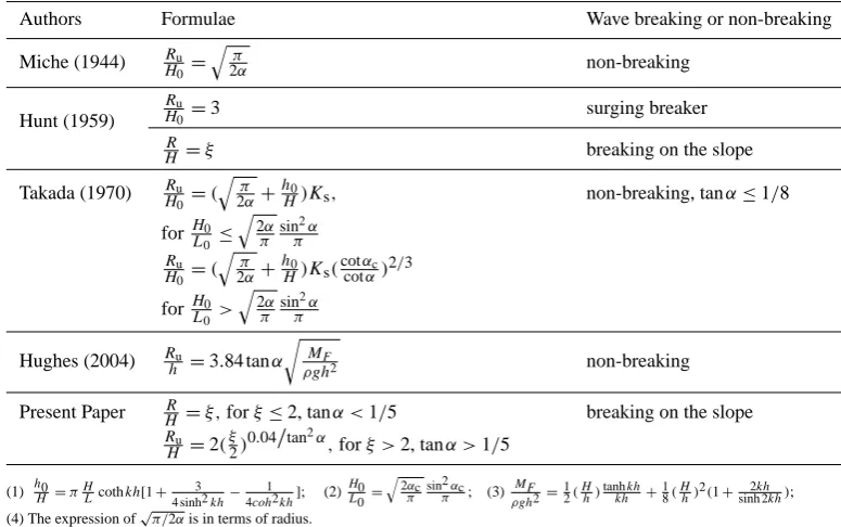
Table 1. Different empirical formulae for regular wave run-ups.
Authors Formulae Wave breaking or non-breaking
Miche (1944) Ru
H0 = q
π
2α non-breaking
Hunt (1959)
Ru
H0 =3 surging breaker
R
H =ξ breaking on the slope
Takada (1970) Ru
H0 =( q
π
2α+ h0 H)Ks,
forH0 L0 ≤
q
2α π sin
2α π Ru
H0 =( q
π
2α+ h0 H)Ks(
cotαc cotα)2/3
forH0 L0 >
q
2α π
sin2α π
non-breaking, tanα≤1/8
Hughes (2004) Ru
h =3.84 tanα r
MF
ρgh2 non-breaking
Present Paper HR =ξ,forξ≤2, tanα <1/5
Ru H =2(
ξ
2) 0.04
tan2α
,forξ >2, tanα >1/5
breaking on the slope
(1) h0
H =πHLcothkh[1+4 sinh23 kh−4coh12kh]; (2) H0 L0 =
q
2αc π
sin2αc
π ; (3)ρghMF2 =12(Hh)tanhkhkh+18(Hh)2(1+sinh 22khkh);
(4) The expression of√π/2αis in terms of radius.
of Stoa (1978), which, in turn, is essentially the same form as Hunt (1959).
Hughes (2004) re-examined wave run-up data for regular, irregular, and solitary waves breaking on smooth imperme-able plane slopes. He presented a new wave run-up equa-tion by introducing a wave parameter representing the max-imum depth-integrated wave momentum flux, as presented in Table 1. Key dimensionless parameters such as the rela-tive wave heightH / h, the relative wavelengthkh(where k
is the wavenumber), and sloping structures tanα, which af-fect the maximum vertical run-up elevation, are included in the equation. Hsiao et al. (2008) presented laboratory exper-imental data from a large wave flume of breaking solitary waves. They used the experimental data to re-examine exist-ing formulae and proposed a simple formula to predict the maximum wave run-up height on a uniform beach with the slope ranging from 1/15 to 1/60.
The abovementioned empirical formulae provide useful information for practical applications, but they are generally limited to a relatively small number of data and to simpli-fied sloping structures. Extrapolation may be required for practical use, but they may be invalid. For example, after several years of practical use, it appears that extreme situ-ations like hurricanes or typhoons are almost never exactly the same as those predicted using these empirical formulae (TAW, 2002). Furthermore, run-up formulae require the rep-resentative wave height and period at the toe of the structures as the input, but when the toe is inside the surf zone, it is difficult to specify the representative wave height and period accurately.
An alternative method for describing wave run-ups on a beach or other structures is the development and application of numerical models that predict temporal and spatial varia-tions of run-up elevavaria-tions. A depth-averaged nonlinear shal-low water equation (Kobayashi, 1989; Raubenheimer and Guza, 1996; Raubenheimer, 2002) is widely used to sim-ulate wave run-ups in engineering practice. However, the model based on a shallow water equation is constricted in the range of long waves or waves propagating in a shal-low water region, i.e., h/L≤1/20, where L is the local wavelength at water depth h. In fact, the general form of Boussinesq equations (BEs) may be sufficient for modeling wave run-up processes over a wider range of water depth re-gions (from deep water depth, h/L≥1/2, to shallow wa-ter depth). For modeling wave breaking, Tao (1983) and Zelt (1991) incorporated the concept of artificial eddy vis-cosity into the momentum equation of BEs. However, the new term for wave breaking did not satisfy the principle of conservation of momentum; this problem was subsequently overcome by Kennedy et al. (2000). Moreover, it has been difficult to combine numerical treatments of wave run-ups – a time-dependent dry–wet moving interface with wave break-ing. Tao (1984) advanced a solution by treating the seabed in the vicinity of a shoreline as a porous media or a narrow slot. Subsequently, Madsen et al. (1997) applied the method of Tao (1984) to BEs, whereas Kennedy et al. (2000) im-proved the solution and satisfied the principle of conservation of mass. For simulating wave run-ups, Lynett et al. (2002) and Nwogu and Demirbilek (2010) developed a numerical model that combined BEs with a dry–wet moving boundary
technique. Fuhrman and Madsen (2008) as well as Mad-sen and Fuhrman (2008) employed so-called extrapolating boundary technique to handle the moving dry–wet interface with a high-order BEs. In addition to the surface elevation, the work established the shoreline velocity which could ac-curately simulate the moving dry–wet interface.
The wave run-up models discussed above are related to run-ups on weakly nonlinear and non-breaking waves. For handling the wave breaking and run-up problems, the current widely used BEs are limited primarily because of their weak nonlinearity (Hsu et al., 2004). Higher-order nonlinear and dispersive equations must be solved for wave breaking and run-ups on a steep structure using a higher-order numerical scheme.
The main purpose of this paper is to report the devel-opment and application of a higher-order numerical model based on the second-order nonlinear BEs derived by Wei et al. (1995) for regular waves. The model developed by Kennedy et al. (2000) was used to model the wave break-ing and run-ups for regular waves. We also performed ex-periments on the run-ups associated with different sloping structures in a wave flume. The evolution of shoreline mo-tions was recorded by using a wire that was installed above the sloping bottom. Laboratory observations were used to validate the numerical results calculated from the BEs for sloping structures varying from 1/5 to 1/3. This verification could confirm the usefulness of the second-order fully non-linear BEs of Wei et al. (1995). Finally, numerical results ob-tained from a series of calculations for regular wave run-ups on a slope from a seawall were obtained, and empirical equa-tions were then derived by regression analysis for practical applications. The equation was also validated by the datasets of Granthem (1953) and Saville (1955). The present paper provides limited but useful information that may be valuable and serve as a stepping stone to investigate run-up predic-tions for irregular wave run-ups on both plane and more com-plex sloping structures.
2 Governing equations and numerical method
Combining the 1-D, second-order, fully nonlinear BEs (Wei et al., 1995) and the modeling method for wave breaking and wave run-ups (Kennedy et al., 2000), the governing equations can be expressed as
ηt= −E(η, u)= −E1+f (x, t ) (1)
Ut∗(u)= −F (η, u)= −F1+Rbx+C1u+C2uxx, (2)
where
E1=
n
Ahu+h2β2/2−h2−hη+η2/6uxx
+(hβ+(h−η) /2) (hu)xx]}x/b (3)
F1=gηx+uux+ {2(hβ−η)u(hu)xx
+(h2β2−η2)uuxx
+ [(hu)x+η ux]2+2η(hu)xt+η2uxt}x/2 (4)
U∗=u+ [h2β2uxx+2hβ(hu)xx]/2 (5)
In Eqs. (3)–(5),u is the horizontal velocity at an arbitrary depth;β=zα/ h, wherezαis the vertical position of an
arbi-trary position; andAandb, the area and width of the narrow slot, respectively, for modeling the wave run-up. The defini-tions ofAandbare from Kennedy et al. (2000). In Eq. (2), the artificial eddy viscosity termRbxis given by
Rbx= ν
t[(h+η)u]x (h+η)
x
. (6)
νt is the dynamic eddy viscosity as a function of time and
space, and it can be expressed as follows:
νt=Bδ2b(h+η)|ηt|, (7)
whereδbis a non-dimensional parameter. A value ofδb=1.2 was proposed by Kennedy et al. (2000) based on the model calibration results.Bis assumed to vary steadily between 0 and 1 to avoid numerical instability for incipient breaking waves. BE model of Wei et al. (1995) is valid for kh<3.8, wherekis the wavenumber. The difference of phase speed between the present model and linear dispersion is less than 2 % underkh < π.
In Eq. (1),f (x, t ) is the wave generating function (Wei and Kirby, 1995):
f (x, t )= (8)
2aexp(k2/4β1)(ω2−α1gk4h3)
ωk√π/β11−α(kh)2
×e−β1(x−x0)2sin(ωt+ε).
In Eq. (2),C1uandC2uxx are the damping terms defined
following Wei and Kirby’s (1995) suggestion. The damping terms are applied to the “sponge layers” that are regions at both ends of the computational domain.
3 Laboratory experiments
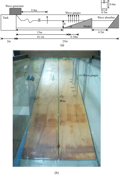
The experiments were carried out in a wave flume at the De-partment of Hydraulic and Ocean Engineering of National Cheng Kung University, Taiwan. The dimensions of the wave flume are 25 m long, 0.5 m wide, and 0.6 m deep, respec-tively. Target regular waves were generated at one end of the flume by using a piston-type wave maker. A plane beach with three different slopes – 1/3, 1/4, and 1/5 (corresponding to 18.43◦, 14.04◦, and 11.31◦, respectively) – was built by us-ing a smooth layer of a wooden model placed atx=15 m starting from the wave board. A preliminary run without any structure was conducted to estimate the wave reflection and to establish the desired amplitude of the incident wave in the wave flume.
A schematic diagram of the experimental setup is shown in Fig. 1. The offshore wave conditions were 1.71 cm≤
H0≤7.26 cm and 0.8 s≤T ≤2.0 s for the wave height and wave period, respectively, which were determined from an automatic wave maker system and adjusted using the first wave gauge located atx=9.9 m by subtracting the reflected waves due to the structure. The water depth was kept constant ath=40 cm, and the wave steepness was within the range ofε=0.003∼0.073, whereε=H0/L0is the wave steep-ness in deep water. Table 2 summarizes the laboratory ex-perimental conditions and measured wave run-ups. The mea-surement apparatus was arranged and deployed with wave gauges and run-up wires, as illustrated in Fig. 1. In order to obtain a higher resolution of the local water surface ele-vation, six capacitance-type wave gauges were deployed at 7.6 cm intervals between 16.1 m<×<16.49 m downstream of the wave maker. The measured data were used to analyze wave breaking, wave profile decay, and run-up height. All the wave gauges were calibrated using a standard procedure in which the water level was changed to adjust the response voltage of each gauge to ensure its linearity and stability. The linear relationship of the gauge response was given by a lin-ear coefficient of 0.99, and this is consistent with the report of Hsu et al. (2002). Each wave gauge had a 16-bit digitiza-tion with noise less than 0.5 mm. The duration of the shore-line motions was continuously recorded by a run-up wire that was installed above the sloping bottom, as shown in Fig. 1b. Note that the run-up wire was enclosed in a plastic tube fixed securely on the sloping bed.
The synchronization of signals from parallel inputs in the wave flume must be considered; hence, to cope with this problem, the data acquisitions of local water surface eleva-tions were recorded simultaneously with a sampling rate of 100 Hz using the multi-nodes data acquisition system (Hsiao et al., 2008).
20
0.38m 15m
16.1m
4.5m
25m 2m
Wave absorber
Model α
9.9m
Wave gauges Tank
Wave generator 0.6m
0.5m
(a)
h
1
(2) Wire
(1) Wave gauges
2
(b) 3
Figure 1. Experimental setup: (a) wave flume and (b) wave gauges and a wire for measuring 4
wave height and run-up.
5 Fig. 1. Experimental setup: (a) wave flume and (b) wave gauges and a wire for measuring wave height and run-up.
4 Model verification
In this section, we verify the applicability of the present nu-merical model by comparing the computed results with var-ious input wave conditions obtained from laboratory experi-ments. Specific attention is given to the spatial variations in wave height and wave run-up height on a slope under wave-breaking conditions.1x=L/100 and1t=T /100 are used for all computations, whereLis the local wavelength andT
is the wave period, respectively.
First, the numerical results (solid line in Fig. 2) for wave height variations (shoaling and breaking) on a 1/20 slop-ing structure are compared with the results of the mild-slope equations (MSE) (dashed line; Hsu et al., 2005) and experi-mental data of Nagayama (1983). In general, the numerical results obtained from the present model agree better with the experimental results than with the MSE, but there is a slight discrepancy for broken wave heights.
A solitary wave of a relative height H0/ h=0.28 prop-agating on a uniform slope of 1:19.85 was also modeled. Computed results were compared with experimental data
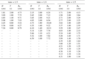
Table 2. Laboratory experimental conditions of wave run-up.
tanα=1/3 tanα=1/4 tanα=1/5
H (cm) T (s) Ru (cm) H (cm) T (s) Ru (cm) H (cm) T (s) Ru (cm) 1.81 3.09 4.85 5.08 4.45 5.36 7.26 – – – – – – – – – – – 2.00 1.80 1.40 1.00 0.80 0.80 0.80 – – – – – – – – – – – 4.73 7.72 9.71 7.93 5.52 6.27 8.79 – – – – – – – – – – – 2.15 2.65 3.65 4.05 4.73 4.35 6.10 5.14 5.66 5.52 6.39 – – – – – – – 2.00 2.00 2.00 2.00 1.80 1.60 1.40 1.20 1.10 1.00 1.00 – – – – – – – 6.24 7.12 9.21 8.56 10.40 9.22 10.21 7.76 4.21 7.02 7.72 – – – – – – – 1.71 1.98 2.71 2.77 3.02 3.37 3.59 4.03 5.24 5.48 3.99 4.29 3.60 4.51 3.79 4.36 5.13 4.31 2.00 2.00 2.00 2.00 1.80 1.80 1.80 1.80 1.60 1.60 1.40 1.40 1.20 1.20 1.10 1.10 1.10 1.00 4.13 3.84 3.29 3.25 2.69 2.55 2.47 2.33 1.75 1.71 1.70 1.64 1.51 1.35 1.35 1.26 1.16 1.16
Note:h=40cm
0 2 4 6
x (m) 0.00 0.05 0.10 H ( m )
(b) slope = 1/20
T = 1.19 sec, Ho = 0.06 m
0.3 m
1
Figure 2. Comparison of the results of wave height distribution along a uniform slope of 1:20 2
among the present numerical model (-), numerical computation using MSE (---, Hsu et al. 3
2005), and the laboratory experiments (●) of Nagayama (1983). Input wave conditions: 4
1.19
T s, H0= 0.06 m, and h0.3m at the toe. 5
Fig. 2. Comparison of the results of wave height distribution along
a uniform slope of 1:20 among the present numerical model (-), nu-merical computation using MSE (–, Hsu et al. 2005), and the labo-ratory experiments (•) of Nagayama (1983). Input wave conditions: T =1.19 s,H0=0.06 m, andh=0.3 m at the toe.
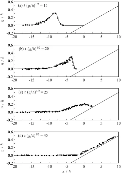
reported in Synolakis (1986). As shown in Fig. 3, the nu-merical results for the water surface elevation at four differ-ent time instances,t (g/ h)1/2=15, 20, 25, and 45, respec-tively, agree well with the laboratory experiments. Lynett et al. (2002) did the same test with COULWAVE, and obtained good results as well. Therefore, the present numerical model is suitable for modeling wave run-up on a sloping seabed for wave breaking and run-up.
Figure 4 shows a comparison between the numerical re-sults and measurements (the symbols for experimental data and numerical results are given in the inset). Note that the predicted wave run-up by the fully second-order BEs model agrees well with measured data for three sloping structures: tanα=1/5, 1/4, and 1/3. Therefore, it will be beneficial to modify the empirical formulae through regression analysis
using the computed results of 160 cases and experimental data and propose an improved formula for practical applica-tions.
5 Results and discussions
The key focus of the present paper is to investigate the wave run-up heights for regular waves breaking on sloping struc-tures. A series of numerical calculations were carried out for regular waves propagating over various sloping structures with the aim of establishing empirical equations for predict-ing wave breakpredict-ing and wave run-up heights. Wave condi-tions including 4 wave periods (T =3.5, 5, 6.5, and 8 s), 16 wave steepnesses ε (0.002, 0.003, 0.004, 0.005, 0.006, 0.007, 0.008, 0.009, 0.010, 0.015, 0.02, 0.03, 0.04, 0.05, 0.06, 0.07), and 10 sloping structures (tanα=1/10∼1/1), totaling 160 cases were simulated. The specified wave steep-ness includes wave nonlinearity and different types of wave breaking. The toe water depthhwas determined under the deep-water condition byk0h=π.
Figure 5 presents the numerical results for different slop-ing structures. It is interestslop-ing to note that the run-up height is highly dependent on the slope of structures. For a given Irib-arren number, the run-up height decreases as the slope an-gle increases. The regression equation ofRu/H=2(ξ /2)m is implemented in the analysis, and it is further expressed by the linear logarithmic regression: log(Ru/H )=mlog(ξ /2)+ log 2, wherem=F(tanα)is the gradient of the linear log-arithmic regression. The coefficient m is shifted slightly
22 1
2
3
4
Figure 3. Comparison of solitary wave propagating from breaking and run-up at four time 5
instances between the present numerical model (-) and the laboratory experiments (●) of 6
Synolakis (1986) on uniform slope of 1:19.85. 7
Fig. 3. Comparison of solitary wave propagating from breaking
and run-up at four time instances between the present numerical model (-) and the laboratory experiments (•) of Synolakis (1986) on uniform slope of 1:19.85.
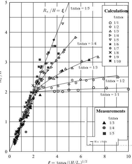
upward from the slope of structures. A more accurate equa-tionm=0.04/tan2αis presented in Fig. 6. We notice that Fig. 6 clearly shows a close relationship between the di-mensionless wave run-upRu/H and the Iribarren numberξ for different values ofm. Figure 7 shows all datasets from numerical simulations and measured data of wave run-ups; herein, the measured run-up data for the rock-bubble struc-ture of slope tanα≤1/5 were taken from Hunt (1959), and the numerical simulations of tanα=1/2 and 1/1 were cal-culated from the BEs of Wei et al. (1995). The remaining are the laboratory data from the present experiments.
The result calculated using the wave run-up height equa-tionRu/H=ξ (Hunt, 1959) is also indicated (solid line for tanα=1/5). It is obvious that Hunt’s equation overestimates the run-up height forξ >2 and tanα >1/5. Notably,Ru/H increases linearly withξforξ ≤2. However, the relationship ofRu/H andξ is very different forξ >2 and tanα >1/5. Under these conditions, as the sloping angle increases, the wave run-up height decreases because of the increase in the
23
Ru
/
H
1
Figure 4. Comparison on the run-up from numerical results with those from measurments. 2 Fig. 4. Comparison on the run-up from numerical results with those
from measurements.
24
2 3 4 5 6 7 8 9 10
2 3 4 5
Slope 1 1/2 1/3 1/4 1/5
m = 0.96
m = 0.634
m = 0.37
m = 0.145
m = 0.04
0 tan / H L/
u
R H
1
Figure 5. Numerical results of R Hu/ versus in logarithmic coordinate for different 2
structure slopes. 3
Fig. 5. Numerical results ofRu/H versusξin logarithmic
coordi-nate for different structure slopes.
downward swash from the fluid weight componentρgsinα, whereρis the density of sea water andgis the gravitational acceleration; this indicates that a steeper sloping structure produces a larger downward force that drags the water rush-ing upwards and results in a lower wave run-up height. The other reason may attribute to surging breakers in which the wave crest collapses and disappears. A considerable amount
25
1 2 3 4 5 6 7 8 910
0.01 0.10 1.00
m
1/ tan
1
Figure 6. The relation between the gradient m and structure slope tan. 2
m
Fig. 6. The relation between the gradient mand structure slope tanα.
of wave energy is released before the toe of the structure, and this results in reductions in the run-up height.
On close examination of the curves shown in Figs. 6 and 7, we conjecture that these curves vary in a nonlinear power form with the slope angle parameter tanαbeing the base pa-rameter. In addition, Goda’s (1975) experiment showed that wave-breaking characteristics are associated with the sloping angle when the waves reach the toe of the structure. There-fore, it is plausible to use the sloping angle as a parameter to distinguish the wave run-up formulae. Note thatRu/H=2 for ξ =2 (Fig. 7) is a branch point of the wave run-up height for various sloping structures. Based on the analyses in Figs. 5 and 6, we performed a nonlinear regression analy-sis using the equation log(Ru/H )=0.04/tan2αlog(ξ /2)+ log 2. The following empirical relationships for a wide range ofξ are thus proposed:
Ru/H=ξ, ξ≤2 or tanα <1/5 (9a)
Ru/H=2(ξ /2)0.04
tan2α
, ξ >2 and tanα >1/5 (9b) In Eq. (9), we use the surf similarity parameter to place the emphasis on the relative importance of wave breaking on a sloping beach. The beach slope is included in an inde-pendent parameter to identify the gravitational effects on the wave run-up on sloping structures. The method used in the present analysis appears to give a more realistic basis by fo-cusing attention on the physical forces as separate terms in the appropriate equation of motion.
The results obtained using Eq. (9) are represented sepa-rately for the first four steep slopes (tanα=1/1, 1/2, 1/3, and 1/4, respectively), as shown in Fig. 7. For tanα <1/5, we notice that Hunt’s formula is still valid with the present derived equation. The correlation coefficient between the computed results from the empirical formula and the data isR2=0.99 for tanα≤1/5, andR2=0.98 for tanα >1/5. Kim and Lee (2009) indicated that Nwogu’s (1993) model results were accurate up to 1:1 slope, but significantly inac-curate for steep slopes. The order of nonlinearity of our BE
26
0 2 4 6 8 10
x= tana/(H/Lo)1/2 0
1 2 3 4 5
Ru
/
H
tana
1/1 1/2 1/3 1/4 1/5 1/6 1/7 1/8 1/9 1/10
Ru /H= x tana = 1/5 Calculation
tana = 1/4
tana = 1/3
tana = 1/2
tana = 1/1
Measurements tana
1/3 1/4 1/5
1
Figure 7. Wave run-up height versus Iribarren number for regular wave transformation on
2
various uniform slopes; the beanch point at can also be seen. 3
─Eq (10)
s
刪除:
Fig. 7. Wave run-up height versus Iribarren numberξ for regular wave transformation on various uniform slopes; the branch point at ξcan also be seen.
model is higher than that of Nwogu’s model. Prediction of our BE model should be reasonable for 1:1 slope simula-tion. Moreover, an agreement indexCR proposed by
Will-mott (1981) is also used to evaluate the confidence of the regression equation, Eq. (10), which is defined as
CR=1−
N P
i=1
(Pi−Oi)2
N P
i=1
Pi− ¯O+
Oi− ¯O 2
(10)
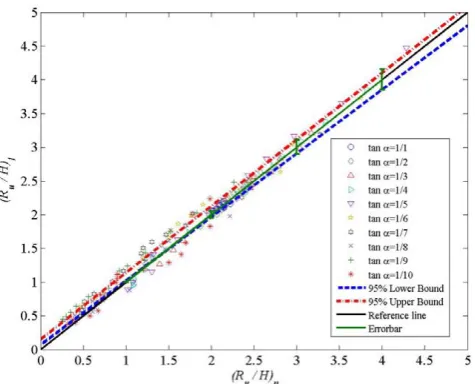
where Pi and Oi denote predicted and observed data, re-spectively; P¯ and O¯, the mean values of Pi and Oi, re-spectively; and N, the total number of evaluated points. The agreement index CR is approximately 0.99. This re-sult shows that the run-up for regular waves predicted by Eq. (10) shows an excellent agreement with the calculated data using BEs and measured data. Precisely defined statis-tical measures of the mean absolute error MAE=P¯− ¯O
,
the root-mean-square error RMSE=
s
1
N N P
i=1
27 1
Figure 8. Correlation and confidence interval between numerical model (Ru /H) and empirical
2
formula (Eq. (10)). 3
Fig. 8. Correlation and confidence interval between numerical
model (Ru/H )and empirical formula (Eq. 9).
indicates that Eq. (9) is able to offer good results for the cal-culated and observed data. Furthermore, good linear relation-ship can be found (Fig. 8) between the numerical results of the present model and those calculated from the empirical equations of Eq. (9). The confidence is in the range of 95 % upper and lower bounds as shown in Fig. 8.
Hughes (2004) re-examined existing wave run-up data for regular, irregular, and solitary waves on smooth and imper-meable plane slopes. A model with a physical argument was used to derive a new wave run-up equation in terms of a wave parameter that represents the maximum momentum flux in a wave as it reaches the toe of the sloping structure. For regular waves, Granthem (1953) and Saville (1955) fitted the equa-tion to regular wave run-ups for all the 152 datasets of labo-ratory tests in which the slopes ranging over 0.1≤tanα≤1 were used in the reanalysis. The empirical formula is given in Table 1. Hughes’ formula reproduces the data trend well, except for Granthem’s results of 1:1 slope, which are lower than estimated. The same data have also been plotted in Fig. 9 using Hunt’s (1959) formula. We note that the Iribarren num-berξ characterizes run-ups very well forξ≤2.0. As slopes become steeper andξ >2.0, the scatter increases. The data trend using linear regression seems to indicate that the branch point is aroundξ=2.5. The formulaR/H=3 was reported by Hunt (1959) for surging breaking, but it significantly over-estimates the wave run-up height.
The proposed run-up relationship of Eq. (9) was further verified using laboratory run-up test results with the same data of Granthem (1953) and Saville (1955). Run-up values for different sloping structures were employed for validat-ing the present formula. For comparison, the wave height at the toe of the structure was estimated by linear shoaling from the measured offshore wave height. The results are pre-sented in Fig. 9. Note that most of the data follow the trend of
28
0.0 1.0 2.0 3.0 4.0 5.0
= tan/ ( H/L0 )1/2
0.0 1.0 2.0 3.0 4.0 5.0 6.0
Ru
/
H
1/3.73 1/2.75 1/2.14 1/1.73 1/1 1/2 1/3 1/6 1/10
tan
tan
tan tan tan
(1)
(1)
(2) Granthem (1953)
Saville (1955)
1
Figure 9. Verification of empirical formulae using datasets of Granthem (1953) and Saville 2
(1955). Line (1) is Hunt’s (1959) formula and Eq. (10a); Line (2) is Hunt’s (1959) formula of 3
/ 3
R H ; others are Eq. (10b). Granthem’s data are given by solid markers and Saville’s 4
data are hollow markers. 5
Fig. 9. Verification of empirical formulae using datasets of
Granthem (1953) and Saville (1955). Line (1) is Hunt’s (1959) for-mula and Eq. (9a); Line (2) is Hunt’s (1959) forfor-mula ofR/H=3; others are Eq. (9b). Granthem’s data are given by solid markers and Saville’s data are hollow markers.
Eq. (9) forξ≤3 and tanα≤1/2, but are overestimated for
ξ >3. On steeper sloping structures, the waves either travel primarily like surging breakers or the downward swash force of waves drags the rushing up water; therefore, the run-up on the slope is reduced. Accordingly, from this comparison, we conclude that Eq. (9) is valid within the range ofξ≤3 and 1/5≤tanα <1/2.
In Eq. (9), it is noted that there is a different measure of wave height at the foot of toe between the experimen-tal dataset generated by the present experiment and those of Granthem and Saville. The wave height at the structure toe was estimated by linear shoaling, but it was calculated by BE model. For a 1:1 structure slope, most of the data have much lower run-up values than estimated. As pointed out by Hughes (2004), waves rushing on this steel slope are proba-bly surging breakers. Madsen and Fuhrman (2008) have ad-dressed this issue recently, and proposed formula for maxi-mum run-up and the associated flow velocity based on theo-retical analysis. So their formulas are valid for a larger value of ξ. Their results also show thatRu/H tends to a unique curve for small ξ, typically following Hunt’s breaking for-mula, whereas a family of curves for various Ru/H exists for largerξ.
Figures 7 and 9 imply that the run-up heights of extreme conditions such as typhoon waves, which may have a larger Iribarren number together with a higher wave height and longer wave period, are generally overestimated by the ex-isting formulae. By comparing Figs. 7 and 9, we can specu-late that the different branch points may be a result of surg-ing breakers or increassurg-ing downward withdraw of the fluid
weight component, or the effect of the opposing current from the down-rush of the preceding crest, in which the wave run-up height is generally overestimated by the previous and present formulae.
The correlation coefficient and agreement index (R2= 0.97 andCR=0.99)between the computed results from the
present numerical model and the proposed empirical equa-tions are high. Hence, Eq. (9) can be useful for practical ap-plications to estimate the wave run-up height for the Iribar-ren number whose range is beyond the conventional value of
ξ=2 but limited toξ ≤3; moreover, the equation can also be useful for test slopes over a wide range from 1/10 to 1/2 for regular waves.
6 Conclusions
In this study, we have applied a numerical model that inte-grates second-order fully nonlinear BEs (Wei et al., 1995) and the analytical theory for wave breaking and run-ups (Kennedy et al., 2000) for simulating wave breaking and the subsequent run-ups for regular waves over sloping structures. Laboratory experiments were carried out in a wave flume for breaking wave run-up on 1/5, 1/4 and 1/3 plane slopes. The property of breaking run-up elevation and its relation-ship with the Iribarren number and sloping structure were discussed.
A total of 160 numerical simulations, using with 4 sets of wave periods with 16 groups of wave steepness on 10 slop-ing structures, were performed. From these data, the wave run-up height for each case was collectively compared with the results of the laboratory results of regular waves. A good agreement was found, with the exception of the discrepancy for surging breakers or sloping structures larger than 1/1 breaking. For a larger Iribarren number and sloping struc-tures (ξ >2 and tanα >1/5), a steeper sloping structure would produce lower wave run-up heights for a given Irib-arren number. The influence of sloping structures on wave run-ups increases due to the increase in the downward swash force from the fluid weight componentρgsinα. This force drags the rushing-up water on a steep slope and reduces the run-up height. A surging breaker could also produce a lower run-up (see Sect. 5).
Alternative empirical formulae are also proposed for the estimation of regular wave run-ups on different sloping struc-tures. The new expression, Eq. (9), is valid for a wide range of the Iribarren numberξ beyond the conventional range of
ξ≤2 (Hunt, 1959), and for sloping structures in the range of 1/5<tanα <1/2. In addition to the existing relationship for wave run-ups on the sloping structures of 1/5, Eq. (9a), a new formula is proposed for sloping structures steeper than 1/5, Eq. (9b).
A precisely defined statistical measure of Eq. (9) was ex-amined. The tests of an agreement measure included the agreement index CR, the mean absolute error (MAE), the
root-mean-square error (RMSE), and the scattering index (SCI), respectively. The results showed that Eq. (9) offers a good prediction compared to the calculated and observed data. The details of the analysis were illustrated in Figs. 5–7. Comparisons and validations of the proposed formulae, using the previous datasets of Granthem (1953) and Saville (1955), and other empirical formulae were shown in Fig. 9.
Based on the model verification, we are confident that Eq. (9) can be applied to the modeling of wave transfor-mations from spilling and plunging wave breaker (ξ ≤3)
run-ups over a wide range of sloping structures with 1/5≤ tanα≤1/2 for regular waves. The present investigation val-idated the model of Wei et al. (1995) for regular waves, and it serves as an important stepping stone to verify irreg-ular waves and more complex geometries of coastal struc-tures. In addition, our results will be very useful to establish good coastal infrastructure protection measures by, for ex-ample, delimiting buffer zones and enhancing the accuracy of coastal risk mapping.
Acknowledgements. The authors acknowledge the support from
National Science Council, Taiwan, under the Grant of 97.2221-E-006-261-MY3 and NSC99-3113-P-006-008. We are especially grateful to the reviewers for giving beneficial comments that were useful for improving the presentation of this paper. Statistical analysis was provided by Ping-Chang Sueh, a Ph.D. candidate of Southampton University, UK.
Edited by: S. Tinti
Reviewed by: two anonymous referees
References
Battjes, J. A.: Surf similarity, Proc. 14th Int. Conf. Coastal Engi-neering, ASCE, 466–480, 1974.
Fuhrman, D. R. and Madsen, P. A.: Simulation of nonlinear wave run-up with a high-order Boussinesq model, Coast. Eng., 55, 139–154, 2008.
Goda, Y.: Irregular wave deformation in the surf zone, Coast. Eng., 18, 15–26, 1975.
Granthem, K. N.: A model study of wave run-up on sloping struc-tures, Technical Report, Series 3, Issue 348, Institute of Eng. Re-search, Univ. of California, Berkeley, California, USA, 1953. Hsiao, S. H., Hsu, T. W., Lin, T. C., and Chang, Y. H.: On the
evo-lution and run-up of breaking solitary waves on a mild sloping beach, Coast. Eng., 55, 975–988, 2008.
Hsu, T. W., Chang, H. K., and Tsai, L. H.: Bragg reflection of waves by different shapes of artificial bars, China Ocean Eng., 16, 343– 358, 2002.
Hsu, T. W., Yang, B. D., and Tseng, I. F.: On the range of validity and accuracy of Boussinesq-type models, China Ocean Eng., 18, 93–106, 2004.
Hughes, S. A.: Estimation of wave run-up on smooth, impermeable slopes using the wave momentum flux parameter, Coast. Eng., 58, 1085–1104, 2004.
Hunt, I. A.: Design of seawalls and breakwaters. Joural of Waterway Harbors Division, ASCE, WW3, 123–152, 1959.
Kennedy, A. B., Chen, Q., Kirby, J. M., and Dalrymple, R. A.: Boussinesq modeling of wave transformation, breaking, and runup, I: 1D, J. Waterw. Port C. Ocean Eng., 126, 39–47, 2000. Kim, G. and Lee, C.: Nwogu-type Boussinesq equations for rapidly
varying topography, Asian Pacific Coasts, 118, 215–221, 2009. Kobayashi, N.: Wave runup and overtopping on beaches and coastal
structures, Adv. Coast. Ocean Eng., 5, 95–154, 1989.
Lynett, P. J., Wu, T. R., and Liu, P. F.: Modeling wave run-up with depth-intergrated equations, Coast. Eng., 49, 291–305, 2002. Madsen, P. A. and Fuhrman, D. R.: Run-up of tsunamis and long
waves in terms of surf-similarity, Coast. Eng., 55, 209–223, 2008.
Madsen, P. A., Sørensen, O. R., and Sch¨affer, H. A.: Surf zone dy-namics simulated by a Boussinesq-type model, Part I: Model de-scription and cross-shore motion of regular waves, Coast. Eng., 32, 255–287, 1997.
Miche, M.: Mouvements ondulatries de la mer en profondeur con-stante on decroissante, Annales des Ponte et Chaussees, 1, 25– 78, 131–164, 270–292, 369–406, 1944.
Nagayama, S.: Study on the change of wave height and energy in the surf zone, Bachelor Eng. thesis, Yokohama National University, Japan, 1983.
Nwogu, O.: Alternative form of Boussinesq equations for nearshore wave propagation, J. Waterw. Port Coastal, Ocean Eng., 119, 618–638, 1993.
Nwogu, O. and Demirbilek, Z.: Infragravity wave motions and runup over shallow fringing reefs, J. Waterw. Port Coastal, Ocean Eng., 136, 295–305, 2010.
Raubenheimer, B.: Observations and predictions of fluid veloci-ties in the surf and swash zone, J. Geophys. Res., 107, 3190, doi:10.1029/2001JC001264, 2002.
Raubenheimer, B. and Guza, R. T.: Observations and predictions of runup, J. Geophys. Res., 101, 575–587, 1996.
Savage, R. P.: Wave run-up in roughened and permeable slopes, J. Waterw. Harbors Div., 99, 1–38, 1958.
Saville Jr., T.: Laboratory data on wave run-up and overtopping on shore structure. Technical Memorandum, 64, Beach Erosion Board, US Army Corps of Engineers, Washington, DC, USA, 1955.
Saville Jr., T.: Wave run-up on shore structures, J. Waterw. Div.-ASCE, 925, 1–14, 1956.
Saville Jr., T.: Wave run-up on composite slopes, Proc. 6th Int. Conf. Coastal Engineering, ASCE, 691–699, 1958.
Shore Protection Manual: US Army Engineer Waterways Experi-ment Station, 4th Edn., US GovernExperi-ment Printing Office, Wash-ington, DC, 1984.
Stoa, P. N.: Reanalysis of wave runup on structures and beaches, U.S. Army Corps of Engineers Coastal Engineering Research Center, Ft. Belvoir, VA, TP 78-2, 1978.
Synolakis, C. E.: The run-up of long waves, Ph.D. thesis, California Institute of Technology, Pasadena, Calif., USA, 1986.
Tao, J.: Computation of wave run-up and breaking. Internal Report, Danish Hydraulics Institute, Denmark, 1983.
Tao, J.: Numerical modeling of wave runup and breaking on the beach, Acta Oceanologia Seneca Beijing, 6, 692–700, 1984. TAW: Technical report wave run-up and wave overtopping at dikes,
Technical advisory committee on flood defence, The Nether-lands, 2002.
Takada, A.: On relation among wave run-up, overtopping and re-flection, Proc. of JSCE, 182, 19–30, 1970 (in Japanese). Toyoshima, O., Shuto, N., and Hashimoto, H.: Wave run-up heights
on coastal dikes, -1/30-, Proc. 11th Japanese Conf. on Coastal Engineering, JSCE, 206–265, 1964 (in Japanese).
Wei, G. and Kirby, J. T.: Time-dependent numerical code for ex-tended Boussinesq equations, J. Waterw. Port Coastal, Ocean Eng. 121, 251–263, 1995.
Wei, G., Kirby, J. T., Grilli, S. T., and Subramanya, R.: A fully linear Boussinesq model for surface waves, Part 1, Highly non-linear unsteady waves, J. Fluid Mech., 294, 71–92, 1995. Willmott, C. J.: On the validation of models, Phys. Geogr., 2, 219–
232, 1981.
Zelt, J. A.: The run-up of non-breaking and breaking solitary waves, Coast. Eng., 15, 205–245, 1991.