Application Of Markovian Probabilistic Process To Develop A Decision Support System For Pavement Maintenance Management

295

Application Of Markovian Probabilistic Process

To Develop A Decision Support System For

Pavement Maintenance Management

Katkar Surendrakumar, Nagrale Prashant, Patil Mayuresh

Abstract: Pavement deterioration rate is very difficult to predict because of the complexities in determining the pavement condition rating or difficulty in collecting detailed data, particularly in absence of sophisticated equipment or trained staff etc. A wide variety of Pavement Maintenance Systems (PMS) are used, but unfortunately either these systems do not use a formalized procedure to determine the pavement condition rating or they assign the pavement state transition probabilities on the basis of experience. The object of this paper is to apply the Markovian probability process of operational research to develop a decision support system (DSS) to predict the future condition of the pavement. Significance of the collected sample data of 20 pavement sections is first tested for Markovian properties. Χ²-inference test is used to check the goodness of fit. Poisson‘s method is used for calculating successive transition matrices for predicting future condition state of pavements. The results support the Markovian probabilistic process tool for finding the future condition states of pavements at any particular year. Improvement in condition of pavement after repair can be easily compared. It will help find the optimal maintenance and repair policy w.r.t. budgetary limits and current state of pavement condition.

Index Terms: Pavement Management, Pavement maintenance and repair, Deterioration modeling, Markovian, Probabilistic Process

————————————————————

1

I

In India, pavement deterioration of pavements is very common. The maintenance of deteriorating or deteriorated pavements is a great challenge to the engineers because of the random features of deterioration process and complex relationship between different parameters. These failures result from the damaging effects of traffic, the environment traffic loading, age etc. As the rate of pavement deterioration is uncertain, the budget requirement at the network level should be treated as this rate of deterioration as uncertain. Modelling uncertainty requires the use of probabilistic operation research techniques. Most of existing Pavement Management Systems use neither a formalized procedure to determine the pavement condition rating nor a deterministic approach to model the pavement rate of deterioration. PMSs use probabilistic prediction models such as Markov models mostly assign the state transition probabilities on the basis of the field staff's experience, which can affect the accuracy of pavement performance prediction.

Deciding the optimal pavement maintenance policy is a challenge to engineers. It needs to address questions such as availability of detailed data, correctness of the data, level of repair treatment to be given, expenses to be incurred on repair, alterative for maintenance or repair strategy etc. Answers to these questions will vary for pavement to pavement. Hence methods to find the repair or maintenance estimate of deteriorated pavements are needed to model which in taking preventive and corrective measures. Greater is the severity of the deterioration, before repair, more will be the repair cost over entire planning horizon. This finding resulted in the definition of a "minimum economical state" before which pavements shall be repaired. This approach permits the identification of the roads to which maintenance should be applied to reduce the added costs caused by delay. The Markov approach allows finding the optimal maintenance decision for pavement in any state, at any given point. The study methodology includes analysis of historical data, the way the pavement deteriorates from year after year, and using it for estimating the transition matrix probabilities. Therefore, the above mentioned system provides the reasonable and practical number of maintenance and rehabilitation plans consistent with the number of deployed condition states.

2.

LITERATURE

REVIEW

Kazuya Aoki (2011) develops the model to estimate the Markovian transition probability. This model is presented to forecast the deterioration process of infrastructure projects. The methodology proposed by him can be applied to forecast the deterioration to some of the infrastructures. Hajek ET. al. (1985) concluded that the measurement and prediction of pavement performance is a cornerstone of any pavement management system. They compared five different prediction methods and suggested that empirical, site-specific models provide the most reliable estimates of pavement serviceability. Khaled A Abaza et.al. (2004) proposed integrated pavement management system with a Markovian prediction model. The study conducted on multi-period planning of maintenance of bituminous pavements. Results are useful to pavement engineers as an effective decision making tool for planning and scheduling of pavement maintenance and rehabilitation work. The developed system applies a discrete-time ————————————————

Katkar Surendrakumar is a Research scholar, Sardar Patel College of Engineering, Andheri (W), Mumbai- 58, India,

PH-09175725910.

E-mail: [email protected]

Nagrale Prashant is a Associate Professor, Sardar Patel College of Engineering, Andheri (W), Mumbai- 58, India, PH-09969056276.

E-mail: [email protected]

Patil Mayuresh is a ME Scholar, Sardar Patel College of Engineering, Andheri (W), Mumbai- 58, India,

PH-09821875163.

296

Markovian model to predict pavement deterioration with the inclusion of pavement improvement resulting from maintenance and rehabilitation (M&R) actions. Kiyoshi Kobayashi et. al. (2008) reported a Bayesian Estimation Method to improve deterioration prediction for infrastructure system with Markov Chain Model wherein estimates of the deterioration process are based upon empirical judgments of Managers at early stages. Worm J. M. et. al. (1995) has designed a DSS for planning of road maintenance used to solve the maintenance problem within budget restrictions. Carnahan et. al. (1987) developed a procedure for making optimal maintenance decisions for a deteriorating system and a methodology is developed to ensure that pavements meet certain performance criteria while minimizing the expected maintenance cost. Literature review revealed that there are various approaches to develop optimal PMS such as mechanistic approach, empirical formulas, probabilistic approach, but to execute; these are quite lengthy and time consuming. There is fair chance of human errors as it includes lots of field work and manual data entry. Observations of pavement condition vary considerably even when such contributing factors are similar. In Indian scenario, where there are no sophisticated instruments and lack of skilled man power; it is highly difficult to assure the correctness of detailed data required by above mentioned processes or approaches. Here in this paper, the condition states are defined in such a way that it accommodates randomness of all depended variables to be incorporated into a pavement management system.

3.

NEED

OF

PAVEMENT

MAINTENANCE

MANAGEMENT

SYSTEM

Pavements are vital elements of transportation network and constitute a significant part of the total construction cost. Overcrowded, overloaded, poorly funded; constructed and maintained pavements cannot be of much use for the development of a country and will increase the chances of accidents, increase vehicular population and various other problems leading to failure of the main purpose of transport system. The beginning of an organized effort for maintenance of highway structures on regular basis has not yet been done in India. Financial constraint has led to initiate the Pavement Maintenance Management System at an early stage. The PMMS in India is in its initial stage of implementation. Despite its importance, pavement maintenance and management has not received proper attention. Absence of proper PMMS leads to faulty investigations of state of pavement condition and hence wrong maintenance or repair policy, ineffective use of budget and dissatisfaction of users. It is mainly because of the misconception that the pavements once constructed need little care and maintenance. IRC special publication, SP: 72-guidelines for inspection and maintenance of rural roads, is the first organized step in this direction.

4.

STUDY

METHODOLOGY

This is one of the most commonly used infrastructure models and has been applied to numerous sequential decision making situations involving uncertainty and multiple objectives. An attempt is made in this study to apply Markovian approach for designing PMMS. Review of Markov theory is presented here that is used in determining transition probabilities and its application in pavement deterioration prediction. The stochastic process is said to satisfy the Markov property if the

future condition of the network is dependent on the present condition of the network and not on its past condition. It alternately means that present state is cumulative effect of all past states. The objective of this investigation is to develop a quantitative approach in the form of mathematical model to represent pavement deterioration based upon a Markovian process and optimal sequence of maintenance expenditures that will satisfy certain performance objectives over a given planning horizon, pavement types, and performance objectives. 20 pavement sections are studied and road condition data is collected. The similar types of roads are taken for the inspection. The pavement life begins at some time in the past, in near-perfect condition – ‗excellent‘ and then is subjected to undergo sequence of duty cycles that cause its condition from ‗excellent‘ to ‗poor‘ from the point of view of usability. The duty cycle for pavement is assumed to be 1 year and all pavement sections carries similar traffic.

4.1 Different Condition States of Pavements

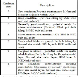
Pavements are classified into seven condition states, from ‗new condition‘ rating 7 till ‗poor‘ rating 1, are presented in Table 1. The description of the condition state of pavement contains all information necessary for decision making.

Table1.Different Condition State Rating of Pavement

DLP: Defect liability period, OGC: Open graded carpet (20 mm thickness), BBM: Bituminous bound macadam (75 mm thickness), Normal size metal layer: Layer of 75 mm thickness of 40 mm nominal size metal, Over size metal layer: Layer of 150 mm thickness of 60 mm nominal size metal.

297

probabilities of one single transition matrix. The state definition given in Table 1 and the next step is to define a vector valued state, i.e.

S



S = the state of every pavement in the system and is a relatively complete description of the state of the system. Using the analogy of pavement deterioration, the starting vector indicates the current condition of the network defined as the proportions in each band of condition. The starting vector shall satisfy the conditions as: The sum of all Si should be equal to one; and all entries shall be non-negative. To model pavement deterioration with time, it is necessary to establish a transition probability matrix, denoted by ‗P‘ in equation (2). The general form of P is given by this matrix contains all of the information necessary to model the movement of the process among the condition states. The transition probabilities, Pij, indicate the probability of the portion of the network in Condition ‗i‘ moving to Condition ‗j‘ in one duty cycle.

4.2 Markov State Definition Process

The different condition states of pavements are given in Table 1. The number of possible states for the description assuming the seven pavement states is 7 N which can be quite large, where N is number of pavements e.g. If there are 3 states (1, 2, and 3) and 2 pavements, then possible description for 2 pavements would be 9 possible states represented as (1, 1) means both pavements in condition state 1. (1, 2) means first pavement in state 1 and second pavement in state 2 etc. Similarly, if there are 5 states (1, 2, 3, 4, and 5) and10 pavements, then there would be approximately 20,000,000 possible states. This would be computationally intractable for any computer. A second modelling approach, termed a counting process, can be implemented which greatly reduces the state space. Consider the above example, where it is assumed that pavements are 10 (N=10) and individual states are five (M=5).

The state space, s = (n1, n2, n3… nm) …. (3) Where,

n1 = the number of pavements in state 1

n2 = the number of pavement in state 2

Σni =N. Then,

|S| =

C

 ₌

C

= 1,001 …. (4) This is considerably more tractable than 20 million. The difference between the two models is loss of individual identity in the second model, i.e. in the second model the state describes the number of pavements in each of the five states and not individual state of each pavement. In general, there is no loss of decision making information in using a counting process model. However, there are thousands of pavements in a system. Counting process gives smaller no. of states than 5N but still significantly large for computation. Hence, the complexity result from the number of states must be reducing. Incorporation of a combination of hierarchical breakdowns into pavement classification and a counting process is needed in order to generate pavement system model where the number of states is computationally feasible. Thus, a more tractable approach is to classify all the pavements into groups that have similar performance characteristics. Pavement performance is dependent upon factors such as pavement type, environmental conditions, traffic loading, age etc. Utilizing those factors, a system of pavements can be grouped into appropriate classes for modelling and for formal data analysis procedures. This classification approach reduces the computational complexity of the pavement network, while providing a tractable representation of the pavement system. Following this approach one can build a Markov model for each of the pavement class, where the state space for each individual model would be Si = (1, 2...5) with cardinality of 5. Such a model would generate a policy for each pavement in the class; however, this approach then requires the integrating via a second – level model of the individual pavement class models. It results in a loss of decision making information. However, the resulting suboptimal design is necessary for tractability of the model and has produced excellent results in numerous models. A second difficulty with such an approach is that only one policy is developed for each pavement class, this issue is easily overcome by allowing the resulting policy (usually randomized) to represent a policy for all pavements in the class.

4.3 Markov Chain Development

298

S (k)



(k)



Then the transition matrix

P = [P ij (a)] = {P [s (k+1) = j | s (k) = i, a (k) = a]}.

The restriction on the transition matrix is that it is stochastic on the transition matrix i.e. the sum of row equal to 1. Once a one-step transition matrix is generated, n-step transition matrices can be generated by matrix multiplication to give stochastic descriptions of future pavement states

4.4 State Transition Sequences

The seven pavement condition states described earlier represents seven possible condition ratings of a particular classification of pavements. It must follow that the deterioration probability of transition from the present to future state is not dependent on past states for the Markovian property to hold that can be written as -

P (j, m | i) = the probability of going from state j to state m, given state i occurred previously to j (i ≥ j ≥ m).

Note that if the Markov property holds then P (j, m | i) = Pjm. An exploratory analysis using field data is developed in the subsequent section to illustrate the verification of the Markovian property. The data related to deterioration of pavement during 1997 to 2011. Data collected year wise for each of the pavements is presented in Table 2. Pavement sections are selected from regions of Daund, Sonawadi, Gar Dapodi, Kedgaon road MDR-82 Tal:Daund, Maharashtra, India. Data is collected from the year of its construction (1997) till 2011. This pavement is found ideal for the research work as there is no maintenance treatment provided since its rehabilitation, except current minor repairs. Major maintenance of the said pavement(s) is not done because the road is parallel to existing railway line and is used only for transport of sand and agricultural goods. Hence it has been given least priority for maintenance. The single pavement length in divided in to 20 sections. The traffic intensity, rainfall, weather conditions will remain same for all of the 20 sections. The whole pavement of 21.8 Km is rehabilitated in different parts as per the availability of funds and priority, and hence these parts are considered as separate pavements for the research study.

299

Each of the cases involves an analysis of two different three-state transition sequences. A three-three-state transition sequence consists of three condition states: past, present and future. These three states correspond to three consecutive pavement condition rating occurring over one year period. Two possible transition sequences, with the same present and future states but different past states are tracked to determine if there is a difference in occurrence dependent of past state history. A simple frequency analysis of sequence occurrence is employed. If there is no significant difference in frequency between the sequences being tracked, this may indicate the Markovian property. An inference analysis using a Chi-square Statistic is also formulated to test the significance of the Markovian property. Not all of the possible state transition can be analysed for Markovian compliance because the available data does not give enough information regarding all possible states. However, transition sequences of the state‘s most frequently occurring in the database are assumed sufficient to establish the Markovian property as it applies to the entire deterioration model.

 State sequence: it refers to a particular three state sequence of concern. This sequence incorporates three consecutive condition ratings of a pavement to establish past- present-future identification.

 State sequence occurrences: it refers to the number of times a specified STS appears in the available database.

 Two-state occurrences: it refers to the number a specified two-state sequence appears in the available database. The two-state sequence involves the past state and the present state. Tracking these occurrences allow for the generation of frequency probabilities as will be described later for example two possible STSs are:(6,6 | 7 ) past = 7, present = 6, future = 6 and (6,6 | 6 ) past = 6, present = 6, future = 6.

The two-state sequence of concern for (6,6 | 7 ) is the transition from state 7 to state 6 while the two-state sequence of concern for (6,6 | 6 ) state 6 remaining unchanged from the past to the present.

Frequency probability: Frequency probability refers to the ratio of SSO over TSO:

P (j, m | i) = Two-stateoccurrences

s occurrence sequence

State

,

P (j, m | i) = [ (i, j)occurrences]

] s occurrence i)

| m (j, [



Here, it is required to calculate future condition states of pavements. The application of Markov process is to calculate future condition states of pavements using the database.

5.

F

A

C

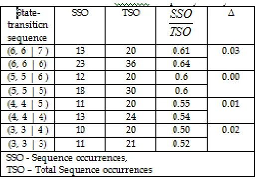
Four cases of state transition sequences are analysed to explore the issue of Markovian compliance. Table 3 gives the question of interest is whether or not the transition from state 6 to state 6 (i.e., no change) is dependent on the previous state6 or 7.

Table 3.Frequency Analysis for Different Past Condition State

If the Markovian property holds, the probability of this transition should be independent of previous state. There are 20 total examples in the database which changes from state 7 (past) to state 6 (present) , and in 13 of these cases pavement remain in same state 6 (future)the following transition was to state 6 (future). Therefore, the probability P (6, 6 | 7) = 0.61. Thus, there is a 61% chance of maintaining state 6 if the previous state was 7. Using 6 as the past state, we get P (6, 6 | 6) = 0.64. Without noise in the data and with perfect Markovian compliance, these numbers should be the same. However, given these difficulties, the probabilities are quite close, with a difference of 0.03.

5.1 Statistical Inference

300

Table 4.Contingency Table for Case 1

The general hypothesis in inference testing is that two disturbances are different. In this scenario, the null-hypothesis is that the generated frequency distributions for a specified case are from the same distribution. Verifying this null-hypothesis based on Chi-squared Statistics gives insight into the concept of accepting the deterioration data a 2x2 contingency table is utilized. For the contingency Table 4, and is referenced to a Chi-square with one degree of freedom to determine the corresponding significance level (α).

χ² = (13+23)(7+13)(13+13)(23+7) 13) + 23 + 7 + (13 )2 23 x 7 -13 x 13 (

= 0.0069 from Table α = 0.947

Table 5. χ² Contingency Table for other cases under

consideration

Similar contingency table generated for other cases and the value of χ² and significance level (α) for each case presented in Table 5.From the result it is observed that there is no reason of rejecting hypothesis. The inference tests for each case indicate that the frequencies are of the same distribution with high significance levels. Also, this influence test further support the suggestion of independence of state deterioration transition on previous states. From above analysis it can be conclude that MDP model is to be developed for a state PMMS, then a similar, more exhaustive procedure must be used to verify the Markovian property. This data analysis is a very positive sign, indicating that the Markovian assumption may be appropriate for other PMMS.

5.3 Development of State Transition Matrices

Various statistical analysis procedures described in the subsequent section, can be utilized for the development of probability transition matrices. The pavement condition data from the available Pavement database is appropriately organized according to the defined condition states. One part of this data quantification process is the classification of the pavements. The second part involves the generation of data matrices for each classification of pavement. The data matrices display the actual number of pavements deteriorating

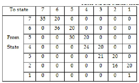
from one state to another with respect to the initial condition states and class. These database matrices are then used in the statistical analysis procedures for the generation of probability distributions for the deterioration prediction modelling of the condition states. The deterioration distribution modelling methodology consists of generating probability distribution for the different rows of a particular data matrix. Table 6 gives the possible future condition states from an initial condition state for the data base shown in Table 2.

Table 6.Data-Matrix from Available Data-Base

As the sample size in first row of Table 6 is greater than 30, a formal statistical analysis procedure is employed.

Table 7.Actual Probability Matrix from Available Data-Base

One such procedure is the utilization of formal probability distributions. Since the data matrices once define seven distinct condition states, discrete distributions are used to model the probability that a pavement at a particular state at the next decision epoch, given the current Pavement state. Such probability functions can be selected using goodness of-fit tests, from numerous possible distributions. One discrete function that provides very useful distribution is the Poisson probability mass function. The given data of the first row is checked for Poisson‘s method. The mean data of observed data is found to be 0.3636 and expected frequency of first row for various value of f(x) is calculated using Poisson Law as,

f(x) = !

3636 . 0 * * 55 !

* 0.3636

x e x

m e

N m xi  xi



301

f (3) = 0.3063,f (4) = 0.0278, f (5) = 0.002, f (6) = 0.00012. These are expected frequencies for first row of Data Matrix. Observed frequency and Expected frequency for other rows are tabulated below

Table 8.χ²-test Result for Goodness of Fit

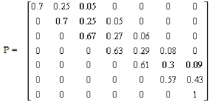
The calculated value of χ² for above first row of data base (0.8729) is much lower than tabulated value of χ² at 5% level of significance and one degree of freedom (3.84). similarly the calculation are made for other rows and results are presented in Table 9 it is indicate, the Poisson‘s distribution can be accepted to test the goodness of fit and can be calculate transition probabilities using expected frequencies of given database. Similar calculation for transition probabilities for other row of transition matrix and arrange in matrix form as:

This transition matrix generated using the aforementioned techniques. The application of matrix chains is used on generated transition matrix to predict deterioration of pavement over time. In this analysis the generated transition matrices represent the probability of an initial condition state ‗i‘ deteriorating to a future condition state ‗j‘ in a one-year period. Therefore, the time interval for the Markov chain is one year.

The multiplication of the transition matrices allows for the probabilistic predictions of future pavement conditions. As expected, if no maintenance is performed, the Pavements were eventually deteriorated to State 1. This is shown by the values of the column for state 1, as further matrix multiplications are made approaching a probability of 1. The generated transition matrices of the deterioration model can, therefore, represent a probabilistic prediction of future pavement conditions. The probabilistic results indicate a range of possible condition states with an associated probability. A deterministic approach, compared to probabilistic results, yields only one potential future value for a condition state. Deterministic approaches may seem limited in the realistic modelling of pavement deteriorations however, they prove useful for comparisons. The expected values are determined from the transition matrix ‗P‘, an initial probability vector P0, and the condition states. The initial probability vector ‗P0‘, represents a priori probabilistic condition of a Pavement. For example, the pavement is new then it is in condition state 7, yielding an initial probability vector P0 = (1, 0, 0, 0, 0, 0, 0). The initial probability vector is multiplied by the transition matrix ‗P‘, generating the vector ‗Pj‘. This vector represents the probability of deteriorating to condition state ‗j‘, given initial probability vector ‗P0‘, for each ‗j‘, ‗Pj‘ can then be multiplied by the condition state ‗j‘, and summed over all ‗j‘. This sum is the deterministic expected value of the condition state. Formally, this process proceeds as follows:

 

P

 

P

P



E (P0) =



 7

1

j 0

}

{

*

j

j

P

…. (9) Where, E (P0) = the expected state of a Pavement in one year given initial probability vector P0.

5.4 Forecasting of pavement condition:

With formulated transition matrix, The future deterioration of pavement after one year, two year, obtained as

 

P

 

P

 

P

 

2

P

 

P

 

P

multiplication can be used for these calculations. The average condition state of any particular pavement in any year can be calculated which gives an overall idea about the pavement condition of total stretch of the road network The deterioration of pavement in successive years represented by equation

E (k) =



 1

7

k 0

}

[P]

)

({P

*

j

j _{.... (10)}

Also calculate the no. of pavements in any particular condition state in a year by equation,

N (k) =



1

7

k 0

}

[P]

)

({P

*

N

j _{.... (11)}

302

N = total number of pavement

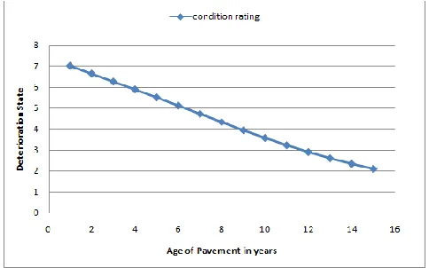
Condition states of future years are shown table (9), includes the average condition rating of pavement at that year and no. of pavements in every condition state. The program is developed in 'C' for easy forecasting the deterioration of pavement.

 The Matrix shown in above table is Transition matrix for that particular year

 Average Condition State is average condition of the pavement at the given year.

E.g. for 10th year it is 3.31 and in 15th year its 1.98

 No. of Pavement column shows the number of pavements in each condition state.

Fig. 1.Deterioration of pavement w.r.t. its age

6.

CONCLUSIONS

1. The contingency table is formulated for different cases for verifying the frequency distribution using χ² test. The test proves that the sample satisfies Markovian properties with high significance level.

2. Using Poisson‘s distribution, one step transition matrix is formulated and used further for calculating successive transition matrices for predicting future condition state of pavements.

3. This study provides a deterministic approach tool to the Markovian probabilistic approach by calculating the future condition states of pavements at any particular year.

4. The study methodology can be used to find overall condition state of complete road network. This helps to compare the improvement in overall condition after repair treatment of a road network. It helps to take correct decision of optimal repair / maintenance policy.

5. The study results conclude that the Markov process is an excellent tool that can be used to design decision support system for Pavement Maintenance Management.

REFERENCES

[1] Carnahan J. V., Davis W. J., Keane P. L., Shahin M. Y. and Wu M. I. , (1987), ―Optimal Maintenance Decisions For Pavement Management‖ , J. ASCE volume 113, page no.554-572.

[2] Kobayashi Kiyoshi, Kaito Kiyoyuki, Letha Nam (March 2012), ―A Bayesian Estimation Method to Improve Deterioration Prediction for Infrastructure System with Markov Chain Model‖, Vol.1, No. 1, page no.1-13. [3] Hajek, Phang J.J., W.A., Prakash, A. and Wrong G.A.

303

[4] Kazuya Aoki (2011)‘―presented Pavement Management, Estimation of Markovian Deterioration Transition Probability‖ page no.1-10.

[5] Chua David K. H., (1996), ―Framework for PMS Using Mechanistic Distress Submodels‖, J ASCE, volume 122, page no.29-40.

[6] Abaza1Khaled A., Ashur Suleiman A. and Al-Khatib Issam A. (2004), ―Integrated Pavement Management System with a Markovian Prediction Model‖, J. ASCE, volume 130, page no.24-33.

[7] Archilla Adrian Ricardo and Madanat Samer (2000), ―Development of a Pavement Rutting Model from Experimental Data‖, J ASCE, volume 126, page no.291-299.

[8] Chen Wai-Fah and Larralde Jesus (1987), ―Estimation of Mechanical Deterioration of Highway Rigid Pavements‖, J ASCE, volume 113, page no.193-208. [9] Indian Road Congress special publication, SP: