How to Do Continuous Stream Processing in a Cloud

(1)

Imperial College of Science, Technology and Medicine Department of Computing

Stream Processing in the Cloud

Wilhelm Kleiminger

Submitted in part fulfilment of the requirements for the MEng Honours degree in Computing of Imperial College, June 2010

(2)

(3)

Abstract

Stock exchanges, sensor networks and other publish/subscribe systems need to deal with high-volume streams of real-time data. Especially financial data has to be processed with low latency in order to cater for high-frequency trading algorithms. In order to deal with the large amounts of incoming data, the stream processing task has to be distributed. Traditionally, distributed stream processing systems balanced their load over a static number of nodes using operator placement or pipelining.

In this report we propose a novel way of doing stream processing by exploiting scalable cluster architectures as provided by IaaS/cloud solutions such as Amazon’s EC2. We show how to implement a cloud-centric stream processor based on the MapReduce framework. We will then design a load balancing algorithm which allows a local stream processor to request additional resources from the cloud when its capacity to handle the input stream becomes insufficient .

(4)

(5)

Acknowledgements I would like to thank:

• My supervisor Peter Pietzuch for the project proposal and his great support and encour-agement throughout the project.

• My second supervisor Alexander Wolf for the insightful discussions on MapReduce. • Eva Kalyvianaki for her help throughout the project and all the great suggestions leading

to this report.

• Nicholas Ng, for proof-reading the script and coming up with the ingenious acronym M.A.P.S. for the custom Python MapReduce implementation. M.A.P.S. stands for “My Awesome Python Script”.

• My sister Lisa for proof-reading and my parents Elke and J¨urgen for their great support throughout school and university. Vielen Dank!

(6)

(7)

Chapter 1

Introduction

Today’s information processing systems face formidable challenges as they are presented with new data at ever-increasing rates [19]. In response, processing architectures have changed with a new emphasis on parallel architectures at the on-chip level. However, research has shown that an increase in the number of cores cannot be seen as a panacea. As cores increase in number and speed, communication becomes increasingly a bottleneck [4]. Alternative solutions like clusters are still preferred for high performance applications. So while the traditional PC has seen advances in multi-core architectures, much of this effort is complemented by a move from local to cloud processing. Cloud-based computing seeks to address the issue that while in most cases today’s computational resources are idling, they may still not be adequate in peak load situations. By sharing resources and requesting more power when needed, we can overcome these bottlenecks. The result should improve both latency and reduce the cost to the user. This projects seeks to evaluate a novel way of load balancing data intensive stream processing queries into a scalable cluster. The goal is to exploit the scalability of a cloud environment in order deal with peaks in the input stream.

Cloud computing has certainly been one of the most hyped trends of the last few years. The result is that companies of tacked this name to a variety of different service offerings. This makes it difficult to come up with a single, concise definition. Kunze and Baun [27] have derived a good definition from Ian Foster’s definition of grid computing [24]:

Cloud computing uses virtualised processing and storage resources in conjunction with modern web-technologies to deliver abstract, scalable platforms and applications as ondemand services. The billing of these services is directly tied to usage statistics. We can distinguish between three applications of Cloud Computing: Infrastructure as a service

(IaaS), Platform as a service (PaaS) and Software as a service (SaaS) [27]. IaaS describes a service that offers computational resources for distributed applications. The infrastructure is flexible enough for the user to run his own operating system and applications. The adminis-tration of the system lies mostly with the user. PaaS takes some of the adminisadminis-tration away from the user and allows some (limited) programming of the resources. An example for this is Google’s App Engine. Finally, and probably most exposed to the general public are SaaS appli-cations. These are offerings such as Apples MobileMe and Google’s email and text processing applications. They offer little to no customisation but the convenience of storing data off-site. We are interested in applying IaaS services to the computation of financial algorithms.

Recent years have seen a massive increase in algorithmic trading. Billions of pounds are traded by software [40]. More than a quarter of all equity trades at Wall Street come down to algorithms

(12)

with little to no human intervention [21]. Financial markets emit hundreds of thousands of messages per second [31]. The exchanges have responded to the demand. The delay between the time a trade is placed and filed at the Singapoore exchange for example has dropped to around 15 milliseconds and other exchanges are following suit [33]. An algorithmic trading systems must therefore process real time data streams with very low latency to in order to stay competitive. The arms-race over ever faster responses to changing market conditions necessitates highly scalable stream processing systems.

Stream processing systems are fundamentally different to ordinary data processing systems. Streams are often too large, too numerous or the important events too sparse [29]. This means data has to be processed on the fly by pre-installed queries. In most cases only a small number of tuples is interesting to the trader. The job of a stream processing system is to find these and make them available in a manner similar to traditional publish/subscribe systems.

A number of systems have emerged to deal with these problems. The distributed systems com-munity coined the term Complex Event Stream Processing for evaluating the output of sensor networks. A similar approach taken by database vendors such as Oracle is simply called Event Stream Processing. The difference between the two is that the former advocates a publish/-subscribe approach [20], whereas the database vendors promote SQL and distributed databases. Current systems distribute the query over a number of nodes [13], thus focussing on the com-plexity of the query itself. We feel that these techniques are too rigid to dynamically scale in a cloud environment. Instead we have chosen to extend the MapReduce paradigm to enable streaming queries.

MapReduce is based on ideas from functional programming. Two functions, map and reduce take over the task of implementing the query. This technology has been successfully employed by Google [19] and others [10] [25] [35] and is supported in by various IaaS providers [5] [6] [7]. As MapReduce has orginally been designed for batch-processing, it will have to undergo some changes to be applied to stream processing. Recently, a first step towards streaming MapReduce has been made with the Hadoop Online Prototype (HOP) [18]. We will build on this work to show how a MapReduce stream processor can be implemented.

The choice to use the MapReduce framework is motivitated by our goal to provide efficient load balancing into the cloud. As we will show later in this report, the data rate of a stream is likely to vary a lot. From our data set, we found the highest demand on the stream processor occurs in the morning, presumably as many trades are carried over from the previous day. The whole trading session lasts 6.5 hours. This is only just over a quarter of a day. Most trading is done on work days. To provide resources 24/7 would not be economical [16]. Instead we opt to design a load balancing algorithm which dynamically responds to bursts in the input stream and relieves the strain on a small-scale, local stream processor by out-sourcing some of the computation to the cloud. The MapReduce implementation on the cloud should then scale as more computational power is required.

(13)

1.1. Contributions 3

1.1

Contributions

In this report we seek to complement the current state of the art in stream processing techniques with the following contributions:

1. Streaming extension for the Hadoop frameworkWe will design and implement the network components necessary to run a streaming MapReduce query on top of the Hadoop framework.

2. MAPS: A Lightweight MapReduce framework written in Python. Starting from the origins of MapReduce in functional programming, we describe the design and imple-mentation of a simple MapReduce stream processor written in Python. The design draws from the lessons learned while working on the Hadoop framework.

3. Loadbalancing strategies to use the cloud in an existing stream processing setup. We show the design and implementation of a minimal version of a single node MapReduce stream processor and how its resources can be complimented by our cloud implementation with two load balancing strategies.

(a) Always-onapproach: The cloud’s resources are always used to complement the local stream processor.

(b) Adaptive approach: The cloud’s resources are used on-demand to assisst the local stream processor.

4. We will evaluate the benefits and limitations of MapReduce for stream processing applications. We will compare our two cloud-based stream processing solutions. Taking the results into account, we will conclude by evaluating our loadbalancing techniques with respect to their ability to assist a local stream processor.

1.2

Outline of this report

In Chapter 2 we will look at existing stream processing solutions, cover the background for our MapReduce implementation and discuss some existing load balancing strategies. We will finish with a short introduction to the financial concepts behind our streaming queries. Having laid the theoretical foundations, Chapter 3 shows how the HOP/Hadoop framework can be extended to process streaming queries. Building on the experiences from the Hadoop stream processor, Chapter 4 focuses on the design and implementation of a custom prototype for a MapReduce stream processor. With a cloud-based solution in place, Chapter 5 focuses on the design of suitable load-balancing algorithms. In Chapter 6, we will evaluate the MapReduce paradigm in the context of financial queries. We will conclude this report by looking at the performance of the load balancing algorithms designed in Chapter 5.

(14)

(15)

Chapter 2

Background

The goal of this project is to enable stream processing in the cloud by using a scalable MapReduce framework. In addition, we are going to evaluate a load balancing algorithm which allows us to utilise the resources of an IaaS provider on-demand. For the purpose of implementation and evaluation we will use a set of local nodes in the college’s datacentre. However, since this is a homogeneous cluster, the results should be easily transferable to a real IaaS service. In order to introduce this ultimate goal of running the MapReduce stream processor with an IaaS provider, we introduce Amazon’s EC2 offering in §2.2.5.

We will start this chapter with a short detour into finance to gain an insight into possible areas of applications of a stream processor and to explain the reasoning behind Put/Call parities -our chosen test query.

After this, we will formally introduce the MapReduce algorithm as designed by Google [19]. The MapReduce algorithm enables data processing on a large number of off-the-shelf nodes. This means that it has now become a focal point of any discussion on cloud computing in general. We will discuss its limitations and why we have initially chosen one of its variations (see §2.3.4) to be part of our implementation. We will then introduce Sawzall, an effort by Google to create a domain specific language for MapReduce and proceed to Hadoop, an open-source implementation of the MapReduce framework. After having laid the algorithmic foundations, we will discuss the underlying infrastructure. Having covered the basics of MapReduce and the underlying platforms, we will concentrate on the current state of the art in stream processing systems and discuss why we have chosen to follow the rather novel path of utilising the MapReduce paradigm. We will conclude this chapter by looking at techniques currently employed in load-balancing and explain how these are applicable to our problem.

2.1

Financial Algorithms

As laid out in the introduction, the financial services industry constitutes a major area of application for stream processing. In our tests we are planning to use stream processing in the cloud to compute financial equations. We have a set of financial data available. This set contains the quotes for options at various stock exchanges for a single day. In order to formulate a sensible query, we must understand the rationale behind the financial data given. In the following we will discuss the concepts behind put and call options as well as the concept of futures trading. At the moment, we are aiming to deploy a single query over the MapReduce network. We must thus formulate a query which makes sense both under the MapReduce as well as financial paradigms.

(16)

2.1.1 Foundations

Options An options contract can be described as follows. Farmer Enno sells investor Antje the right to buy next year’s harvest at a specific strike price. Obviously, neither knows the actual value of the harvest. Enno produces biofuel. Now say the economy dips into recession the following year and substitute goods such as oil become cheaper. Then Enno’s biofuel will drop in price as well and Antje is going to drop her option. She has lost the commission and any other associated fees. However, if the economy is well and Enno has an exceptional harvest, Antje will exercise her option. The price of the option is below the actual market price. Antje will be able to sell the fuel at a premium.

Futures In contrast to options, futures are binding contracts over the purchase of a good. If Antje buys a futures contract on Enno’s harvest, she is obliged to buy it at the spot price. This guarantees Enno a specific price for his harvest and insures Antje against rising costs. Our dataset only includes options data and thus we will not discuss futures any further. Below we define a few financial terms necessary for the further discussion.

Short selling A buyer borrows a position (eg. shares) from a broker, betting its price will fall. The broker receives a commission. The buyer immediately sells the position (going short). With prices falling, the buyer can now re-acquire the position and return it to the broker. The buyer has made a profit of the difference between the initial sell and final buy actions minus the commission. The buyer makes a loss if prices rise as he has to buy at a premium to his initial sell price.

Long buying This is the opposite to short selling and describes buying positions and betting that prices will rise in future.

Bonds Bonds are similar to shares. Shareholders are owners of the company and shares can be held indefinitely. Bondholders are creditors of the company and bonds are usually associated with a due date. This time period is called maturity. As shares usually pay dividends, bonds have an associated interest rate called coupon.

2.1.2 Put and call options

In options trading we distinguish two types of financial produces. Put andCall options. Put and call options are short selling and long buying applied to options. If Antje thinks that the price of Enno’s harvest will decrease in future, she can buy a put. A put means that Antje is going short on the right to buy Enno’s harvest. Should the weather outlook dictate a higher price for the option, Antje will have to buy back the option at a premium and therefore lose money. However, if prices of biofuel seem likely to fall, Antje is most likely to be able to buy back the option at a cheaper price and return it to the broker at a premium. In options trading, the seller, previously referred to as broker is called writer. Obviously, the writer’s profit is maximised if the buyer chooses not to exercise the option.

A call option is the name for acquiring the right to buy shares of stock at a specific strike price in the future. In the above paragraph on options, we have described this simple case of options already.

(17)

2.1. Financial Algorithms 7 2.1.3 Arbitrage opportunities

Put-call parity

Put-Call parity is a relationship between put and call options which mainly applies to Euro-pean options1

[12]. This concept is important for valuing options but can provide a arbitrage opportunity.

Portfolio A We define the following variables for the put: • KStrike price at time T

• S Share price on day of expiry (unknown constant at time T)

Now, assume we have a portfolio with a single put position at strike priceK (short option) and a single share at time T. Should the (unknown) share price S, be the same or exceed K, the value of our portfolio is S as we do not wish to exercise the option. Should the strike price, however, be greater than S we would like to exercise the option and our portfolio is worth the value of the put, K−S plus the value of the shareS: K−S+S =K.

Portfolio B For the call we define the following variables: • KK bonds each worth 1 unit (constant value)

• S Share price on day of expiry (unknown constant at time T)

A portfolio with a single call position (normal option) andK bonds (each worth 1) is worth the same as A if their strike price and expiry are the same. K always remains the same. Like above if at time T, the strike price K is less than the (unknown) share price S, we wish to exercise the right to buy stock at K and make a profit ofS−K. The total value of our portfolio in this case is S. If the strike price K is greater than S, we will chose not to exercise the option and therefore have a portfolio worth K. This shows that at time T, both portfolios have the same value regardless of the relationship between T and S.

If one of the portfolios was cheaper than the other, then there would be an arbitrage opportunity since we could go long on the cheaper one and go short on the more expensive one. At the expiration T the portfolio will have zero value. But any profit made before is kept.

Relation to our project For our purposes, when we talk about ”put-call parity”, we simply wish to find out if we can find two markets with a put and a call options at the same strike price and with the same expiry date. As we do not have any information about the rest of the market, we cannot evaluate the financial formulae using prices for bonds, shares and dividend/coupon payments. We envisage that the full implementation will be possible in a system using multiple queries.

1

(18)

2.2

Cloud computing

2.2.1 MapReduce

MapReduce was first introduced by Google in 2004 [19]. It is a framework designed to abstract the details of a large cluster of machines to facilitate computation on large datasets. The inspiration for the MapReduce concept was taken from functional programming languages such as Haskell. Nowadays, many companies have implemented their own MapReduce frameworks. Open source implementations exist. In the following we will describe how MapReduce works and how it can be applied to our task.

Google File System (GFS) MapReduce works by distributing tasks over a large number of individual nodes. Therefore, the implementation is often accompanied by a distributed file system. In the original Google implementation this is GFS [19], the Google File System. GFS is particularly suited for MapReduce as the framework assumes that files are large and updated through concatenation rather than modification. In GFS, files are divided into chunks of 64MB each and then distributed across several chunk servers [39]. Replication is used so that we can recover from failures such as a machine becoming disconnected from the network.

How it works The main goal of MapReduce is to prevent the user from creating a solution that requires a lot of synchronisation. All synchronisation is done within the MapReduce framework. This way we avoid the pitfalls induced from race conditions and deadlocks. We can focus on the actual computation of values. In order to simplify data handling, the programming model also specifies the input and output as sets of key/value pairs.

The MapReduce algorithm then follows a divide and conquer approach to compute a set of output pairs for a given set of input pairs. This is done through two functions: Map and Reduce. Using the divide and conquer approach, the master node distributes the input tuples over the set of worker nodes by splitting the problem into a smaller sub problems. The map phase can form a tree structure in which problems are recursively split into smaller sub-problems before being passed to the reduce phase. Similarly, the output of the reduce phase can be fed back into the system and start another map reduce iteration. The necessary work is done within the MapReduce library.

In Haskell notation, one would describe the map and reduce functions in the following way:

map :: (key_1, value_1) -> [(key_2, value_2)] reduce :: (key_2, [value_2]) -> [value_3]

The map function takes a (key, value)pair and produces a list of pairs in a different domain. The framework takes these pairs and collates values under the same key. The resulting pair of (key, [value]) is then processed by the reduce function to produce output values in a (possibly) different domain. The original C++ implementation uses string inputs and outputs and leaves it to the user to convert to the appropriate types. The following map and reduce functions illustrate how the MapReduce framework can be used to count the occurrences of each word in a large set of documents.

This example mirrors the working of the map and reduce functions. For each word, the map function emits a tuple with the word as the key and the number 1 as its value. As the reduce

(19)

2.2. Cloud computing 9

1 _def _{map ( name , document ) :} 2 f o r word in document do 3 _{E m i t I n t e r m e d i a t e (w, 1 )} 4 5 _def _{r e d u c e ( word , p a r t i a l C o u n t s ) :} 6 _{r e s = 0} 7 _{f o r} _pc _in _{p a r t i a l C o u n t s :} 8 _{r e s = r e s + pc} 9 _{Emit ( r e s )}

Listing 2.1: MapReduce Example

function is operating on all values of a single key, it just sums up the 1’s from each individual word and returns the total number of appearances. The partialCounts variable is an iterator which walks over the output from the map function as written to the distributed file system. Besides the map and reduce functions we further have an input reader which reads from the file system and produces the input tuples for the map function. These tuples are split into a set of M splits and processed in parallel by the worker nodes. The partitioning for the reduce nodes is similar. We specify a partitioning function like hash(key) mod R to do this. The partitioning function is used to split the data into R regions when buffered data from the map tasks is written to stable storage. The master is notified and then notifies the reduce tasks to start working. Because the hash function can map multiple keys to one region, we need to sort the data at the reduce node before we can process region R. Finally an output writer takes the output of the reduce function and writes it to stable storage.

In some cases it is advisable to put a combiner function in between the map and reduce stages to limit the amount of data passed on to the network layer. This can be seen in the word counting example, where given the input language of the documents is English, there will be a lot of

("the", 1)pairs emitted. The combiner function acts like the reduce step, the difference being that the algorithm writes its output to an intermediate file, whereas the output of the reduce step is written to the final output file.

As is tradition with Google, MapReduce clusters typically consist of large clusters of commodity PCs networked via ordinary switched Ethernet. Network failures are common, therefore, the algorithm has to be very failure tolerant. By ensuring that individual operations are independent, it is easy to reschedule map operations in case of failure. However, we must be more careful when output of a failed map has already been partially consumed by a reduce operation. In this case the reduce has to be aborted and rescheduled, too.

So far we have assumed that the map and reduce operations are independent. This restriction allows us to make full use of the distributed system as these operations can all be executed in parallel without any significant locking overhead. The restriction is that the data has to be available to the processing units without any significant delay. In the original implementation, a reduce task for example needs all the data for a particular key to be presented at the same time. To be able to process streams efficiently, we need to get rid of this restriction. As this restriction was implemented using a write to the distributed file system GFS, we need to stream data from mappers to reducers instead. The details of this are discussed in§2.3.4.

Criticism / Evaluation Our choice in favour of MapReduce is motivated by the ease of use of its programming model and the tight integration with the cloud paradigm. The MapReduce design provides natural support for scalability with its mappers and reducers. However, there has been some criticism voiced over its implementation. Notably, David DeWitt and Michael

(20)

1 _{count : t a b l e sum o f i n t ;} 2 _{t o t a l : t a b l e sum o f f l o a t ;} 3 _{s u m o f s q u a r e s : t a b l e sum o f f l o a t ;} 4 _{x : f l o a t = i n p u t ;} 5 _{emit count} <− 1 ; 6 _{emit t o t a l} <− x ; 7 _{emit s u m o f s q u a r e s} <− x ∗ x ;

Listing 2.2: Sawzall Example

Stonebraker, two proponents of distributed databases have criticised MapReduce for its lack of expressiveness [22]. They argue that the programming model is outdated and not able to utilise any of the performance improvements known from traditional databases such as indexing. We argue that although DeWitt and Stonebraker are right on the limited expressiveness, they miss the point on the purpose of MapReduce. MapReduce is an excellent way to process a large amount of data that comes in a relatively unstructured form. Once we have processed the data, we can store it in relational tuples and evaluate it further using a traditional database approach. The two approaches are therefore complimentary, a result that Stonebraker et al. acknowledge in a later paper [36]. They refer to the pre-processing stage as extract-transform-load tasks and call them a MapReduce speciality. In our project we will evaluate relational tuples as we expect the difference between MapReduce and distributed database systems to be negligible in single-query environments.

2.2.2 Sawzall

DeWitt and Stonebraker also criticised MapReduce for its lack of high level query language. Recently, there have been several efforts to remedy this. Sawzall is a domain specific procedural language developed by Google to lie on top of the MapReduce framework. This language takes the MapReduce approach further to make sure that its programmers write parallel code. It uses a set of aggregators “to capture many common data processing and data reduction problems” [34]. As Sawzall is an interpreted language, we might think this would pose a significant constraint in a high performance environment. However, as the algorithms mainly spend time on I/O and the underlying methods are implemented natively, this does not incur any significant penalty. The increase in performance when adding machines is almost linear. As we need more control over the communication between the hosts to implement our stream processing paradigm, we cannot use Sawzall to program the cloud infrastructure. However, this is an interesting approach and it might be considered to extend Sawzall to enable stream processing as the authors suggest. The following simple Sawzall program (Listing 2.2) takes as input a set of records containing one floating point number each. It then produces three results. The total number of records, the sum of all the floating point values and the sum of the squares of the floating point numbers. This looks very similar to the map phase as we have seen in the discussion of MapReduce in §2.2.1. Here we define three aggregators: count, total and sum of squares. By defining these aggregators as sum tables we tell Sawzall what the reduce part of MapReduce should be doing. By pre-defining the aggregators, Sawzall relieves the programmer of the reduce task but also somewhat limits the expressiveness of map reduce. However, the upside is that the aggregators can now be implemented natively. Furthermore, the parallelism is hidden from the user. Aggregators have to be commutative, associative and efficient for distributed programming. Extending the set of aggregators is therefore difficult.

(21)

2.2. Cloud computing 11 Evaluation Sawzall is a very interesting approach to take MapReduce more en par with traditional database systems. By designing a domain specific language it is possible to further abstract and simplify parallel programming. At this stage, Sawzall is not yet able to express streaming queries. However, we will keep MapReduce DSL approaches in mind for further projects.

2.2.3 Hadoop

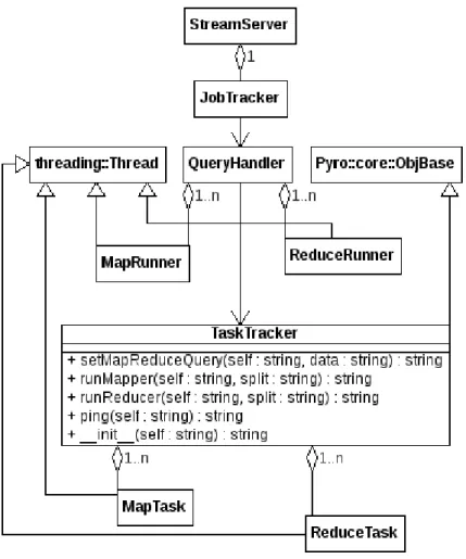
Hadoop is the umbrella project for several Apache projects which have the aim to provide a reliable platform for distributed computing. The Hadoop project can be split into two parts. The first is an implementation of MapReduce. Although the framework is written in Java, it accepts MapReduce tasks written in other languages [1]. Similarly to Google’s Sawzall effort, the Hadoop project also includes Pig [28], a high level data-flow language to describe parallel processes. Pig’s compiler produces a chain of MapReduce operations. The language layer is called Pig-latin. The second part of the Hadoop implementation is the Hadoop Distributed File System (HDFS), a file system, similar to GFS as employed in MapReduce [19]. Both HDFS and GFS are optimised for batch processing.

Figure 2.1: Hadoop implementation

Architecture

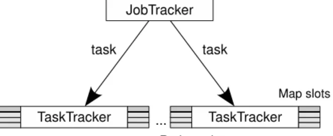
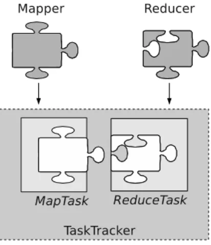
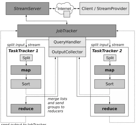
Fig.2.1, shows the organisation of a Hadoop installation. The master node is called JobTracker

and waits for incoming jobs. The jobs are split into tasks and assigned to worker nodes - called

TaskTrackers. A TaskTracker has a fixed number of slots to run map and reduce tasks. The execution of these is managed by the TaskTrackers themselves. The JobTracker uses a heartbeat protocol to keep record of free slots on the TaskTrackers and to schedule new tasks [18].

Hadoop job submission

A new MapReduce job is submitted through the JobClient interface. The JobClient provides facilities to monitor the MapReduce cluster, submit jobs and view their status. When a job is submitted to the JobTracker via the JobClient, the following steps are executed [2]:

1. Checking input and output configuration. 2. Computing the InputSplit2

values for the job.

2

(22)

3. Copying the job’s jar and configuration to the MapReduce system directory on the file system.

4. Submitting the job to the JobTracker and monitoring its status.

Evaluation Hadoop is available on as cloud images and a standalone application and therefore interesting to our project. This and the amount of supporting tutorial material for Hadoop convinced us to choose it for the MapReduce implementation. In its original design it does not allow for streaming MapReduce. This limitation is covered in§2.3.4.

2.2.4 Remote Procedure Calls

As distributed systems like Hadoop have to communicate intermediate results and to coordinate their behaviour, they need a reliable way to communicate. In Hadoop, a lot of inter-process communication is done using RMI, the Java version of a Remote Procedure Call (RPC). RPC is a technology to lookup functions outside the address space of the current process [30]. This could mean a function on the same node, implemented by a class running in a different process, or code running on a different machine altogether. In either case, once the function has been bound by the RPC framework on the local machine, a call behaves (almost) exactly like you would expect it to on a local machine.

Implementation

A remote procedure call initialised and executed through message-passing [39]. The client node first sends a request to the server process containing a unique identifier for the function to be called. In order to find the server implementing the function, the calling process might either broadcast a message on the local network or request a list of implementations from a well known name server. In the latter case, it is necessary for the server process to register its implementation first. Once the client has completed the lookup phase for the particular function, it is bound to a local stub and can be used by the rest of the program. On the server side, a daemon ensures that all communication request are dealt with by either spawning a new thread or picking one from a pre-initialised thread pool.

Serialisation

RPC libraries can easily deal with most basic data types such as integers and strings. However, if we wish to call methods on complicated objects by reference, we need to make sure that the remote host is aware of these objects first. We need to serialise the object [39]. Serialisation of an object such as a linked list means traversing all the pointers and essentially flattening the datastructure such that it can be either saved to disk or transmitted over the network. Flatting complex datastructures is not always an easy task as we must follow all references without looping forever due to back edges in the graph. Furthermore, we cannot merely send the contents of the objects over the network as any pointer variables will not have the same meaning on a remote host. The solution to this problem is called pointer swizzling. In our example of a linked list, we would for example introduce a new field to every node holding a unique identifier. We can then set the pointer to the next node to its identifier rather than the address in memory. This process can be easily reversed at the other side. However, there is an cost associated with this operation. Thus, serialisation should not be used extensively

(23)

2.2. Cloud computing 13 when communicating in an environment where runtime is critical. When applicable, simpler datastructures should be used.

Java RMI

Remote method invocation (RMI) is Java’s implementation of the RPC protocol. Instead of publishing information on a single method with a nameserver, the callee registers its remote object with the RMI-Registry under a unique identifier [37]. The client program can now query the RMI-Registry with this identifier to get a reference to the remote object. This reference has to be an implementation of its remote interface. The remote interface defines the methods that are guaranteed to be implemented by the remote object. The client can now call the methods on the remote object as published by the remote interface. It is possible for the method headers of the remote object to contain references to interfaces. Any class implementing these interfaces may then be used on the remote host including class definitions from the caller. This means that Java gives the user the opportunity to dynamically load new code as part of a RMI call. In order to make sure that this is not exploited for malicious use, a security manager is always installed as part of the RMI implementation. Any special requests have first to be granted by the designer of the server application.

2.2.5 Amazon EC2

Despite having chosen to implement our stream processor on cluster nodes in the college, our ultimate aim is to run stream processing on an IaaS platform such as Amazon EC2. The decision to develop and test locally has been purely a development one. However, as all our machines are single-purpose and only used for this project, our setup is not too dissimilar to a “cloud”. The participating nodes are running the same specifications. In fact, the EC2 technology is available as part of the Ubuntu Eucalyptus packages and can be integrated into an Ubuntu server installation. It could thus be easily installed on our test cluster.

Amazon’s EC2 offering, introduced in 2006 [11], was one of the first commercial cloud infras-tructures. EC stands for Elastic Cloud. Customers are allowed to create an Amazon Machine Image. This image is used to start a virtual machine on the Amazon cluster. The infrastructure allows customers to start and terminate new virtual machines as required by the application, hence the term elastic. Additional nodes can be accessed within minutes. This ease of use makes it very interesting for our purposes of load balancing. Amazon charges by the hour or the data transfer rate. Further charges are possible. The various virtual machines instances as of December 2009 are shown below. These instances are based on the notion of EC2 Compute Units. The units mirror equivalent capacity of physical hardware. It is possible to specify the geographical location of the servers in order to optimize network latency and fault tolerance.

1. Small Instance (Default) 1.7 GB of memory, 1 EC2 Compute Unit (1 virtual core with 1 EC2 Compute Unit), 160 GB of local instance storage, 32-bit platform

2. Large Instance 7.5 GB of memory, 4 EC2 Compute Units (2 virtual cores with 2 EC2 Compute Units each), 850 GB of local instance storage, 64-bit platform

3. Extra Large Instance 15 GB of memory, 8 EC2 Compute Units (4 virtual cores with 2 EC2 Compute Units each), 1690 GB of local instance storage, 64-bit platform

(24)

The Amazon CloudWatch service gives information about the current load on the system. This information can be accessed via a web service or web APIs. Unfortunately, this service incurs a charge for the number of monitoring instances used. However, the CloudWatch service is necessary for using the auto scaling feature of EC2. Auto-scaling enables us to specify triggers which cause Amazon to add or remove instances automatically.

Persistent storage on EC2 systems is provided using the Amazon Simple Storage (S3) service. The EC2 implementation itself only stores temporary data. If an instance is rebooted, this data is lost. As this can happen explicit via an API call or a failure in the system, we cannot ensure fault-tolerance without a form of persistent storage. Google’s MapReduce algorithm requires a distributed file system to store the intermediate results. The S3 service makes data available directly to the EC2 instances and over the network via http. This makes it suitable for ordinary MapReduce. For low latency access, we must use S3 and EC2 services in the same area. There is no extra cost for S3 to EC2 bandwidth. Despite its advantages and close link to the original MapReduce idea, the distributed file system is more of an obstacle towards efficient stream processing as both input and output should be written to sockets rather than to stable storage.

2.3

Stream processing

In this section we are covering several research prototypes of stream processing, ranging from single node implementations to distributed versions. The goal of the project is to focus on the load-balancing between the front-end node and the processing power of the cloud. In this light, we will evaluate the state of the art and rationalise our decision to use a MapReduce framework to do stream processing in a cloud environment.

2.3.1 Mortar

Logothethis and Yocum have developed Mortar - “A distributed stream processing platform for building very large queries” [29]. The Mortar platform focuses on applications with thousands of distributed sources. It takes into account unreliable sources and adverse network connections. Mortar is designed to manage streaming queries across large federated systems3

. The Mortar infrastructure takes over the task of creating and removing operators as well as organising the data flow between them. For this reason, one of the main contributions of the above paper is to provide robust overlay networks to run queries. Mortar also addresses the problem of time synchronisation between the different nodes. Stream processing cannot work without reliable time information as the timestamps used for windows become useless. Mortar differentiates itself from the other approaches shown here, as not only are the data-supplying nodes involved in the processing, but the designers want them to be the only ones to do the work. Logothetis and Yocum speak of scoped queries in this context. We now discuss the overlay networks and routing algorithm employed by Mortar.

Overlay network The overlay networks in Mortar are static. The authors justify this by the claim that in federated systems, machines are rarely added or removed. They can only become unavailable for a short time. It is assumed that there is personnel in charge of the sites which quickly rectifies any problems. However, in order to deal with failures, multiple static trees are created and operators are connected across them. The static aggregation trees in the Mortar framework are build such that the majority of nodes is close to the root node.

3

(25)

2.3. Stream processing 15 This is necessary to ensure the latency bounds required by streaming applications. Once the primary tree is built, the sibling trees are derived through successive random rotations of internal subtrees. The authors have confirmed by empirical observation, that this is unlikely to change the clustering.

Dynamic tuple striping The routing scheme proposed by Logothetis and Yocum is called

dynamic tuple striping. Dynamic striping is a multi-path routing scheme. Routing is done up the trees towards the root. Since scoped queries are used, each node needs to know about all live parents for locally installed queries. These are found using a heartbeat protocol. Children are updated in the same way. Tuples are routed through a parent only if this moves them closer to the root. The algorithm first tries to use the parent on the tree on which the tuple arrived. If this fails, it tries a parent on a different tree which must not be further away from the root as the current tree. This avoids cycles. However, if no further progress could be made, a tuple is allowed to move down to a child and try a different path. As this now introduces the possibility to incur cycles, a time to live field is introduced (TTL) to restrict the number of tries.

Evaluation Mortar has somewhat limited applicability to our cloud approach. As our chosen platform is homogeneous and under a single administration we have eliminated most of the problems stemming from federated systems. Indeed, the implementation of our chosen stream processor should be modifiable to run on virtual machines which might be added or removed during the computation. This form of scalability is not what the authors of Mortar envisaged. Mortar is a very reliable platform for applications such as sensor networks with a large number of data providing nodes. In these cases an overlay network is justified. In our case, however, it violates the low latency requirements. Applying Mortar to stream processing in a cloud setting would require too many modifications.

2.3.2 STREAM

STREAM is a data stream management system (DSMS) developed by the University of Stan-ford [9]. Ordinary database management systems (DBMS) deal with one-time queries. Network monitoring, financial analysis and sensor networks, however, emit a continuous stream of data. Thus in addition to ordinary relations, we have bags of tuple, timestamp pairs, called streams. Streams can only be handled by continuous queries. The STREAM project aims to fill this gap. The prototype DSMS [9], supports a “large class of declarative continuous queries over continuous streams”. It evaluates the queries by translating the declarative queries into a phys-ical query plan. This plan is then processed by the DSMS. A query plan consists of operators, queues and synopses.

Operators Arasu et al. have developed the Continuous Query Language (CQL) [9]. CQL looks very much like an extension to SQL. There are three types of operators: relation-to-relation, relation-to-stream and stream-to-relation. The relation-to-relation operators are the well-known SQL operators. The stream-to-relation operators are more interesting. They offer the ability to turn the continuous stream into a relation which can be modified by ordinary relational algebra. The stream-to-relation operators are following the sliding window concept. Atuple-basedsliding window is expressed using[ROWS N]after the steam identifier. This returns a relation with the last N tuples/rows in the stream. The [Range N] parameter gives a time-based sliding window. The relation returned includes all tuples with more than N timesteps in

(26)

1 _{S e l e ct} _{IStream (}_∗₎ _From _{S [}_Rows _{1 0 0 ]} _Where _{S .A} > 10

2 S e l e ct IStream (∗) From S [Rows Unbounded ] Where S .A> ₁₀

3 _{S e l e ct} _{IStream (}_∗₎ _From _{S [ Range 1 0 ]} _Where _{S .A} > 10

4 S e l e ct IStream (∗) From S [ Now ] Where S .A > ₁₀

Listing 2.3: New operators in CQL

the past. The abbreviation [Now] returns the window with N = 0; i.e. only tuples that have the same timestamp as the clock of the DSMS are returned. Examples are shown in Listing 2.3. The last type of stream-to-relation operators is a little more complex. A partitioned sliding window, takes a set of attributes over which it splits the input stream into separate substreams

[Partition by A,...,Z ROWS N]. N specifies the number of rows used in this process. The individual windows are combined using the SQL union operator to generate the output relation. If we want to turn the output relation back into a stream, we can userelation-to-streamoperators. CQL defines three relation-to-stream operators. Istream or insert stream, contains all the tuples inserted into the relation. Every time a new tuple is added to the relation, it is forwarded to the stream (unless it is a duplicate). Dstream or delete stream, contains all the tuples deleted from the relation. Like for the insert stream, deleted tuples are forwarded to the stream. Rstream or relation stream contains all tuples in the relation at all time instants. The first line of Listing 2.3 therefore selects 100 rows from the stream S, turns it into a relation, selects all tuples where

S.A >10 and returns these as a stream.

Queues As queries are converted to physical query plans, we need queues between the opera-tors. Queues are connecting the operators and can be empty. Due to the nature of the processing, queues have to be read in non-decreasing timestamp order. Only this way, an operator can be sure that all the necessary data is present to close the window and begin processing.

Synopses Synopses are associated with operators and further describe the data. An example given by Arasu et al. is that of a windowed join of two streams. In this case the synopsis are a hash table for each of the input streams. A synopsis can be shared amongst multiple operators.

Evaluation The STREAM project has led the way in the field of stream processing. The expressiveness of CQL is great and the available optimisations manifold. Arasu et al. [9] identify operator reuse and replication as two performance enhancing components of placement algo-rithms. This is because in large static queries certain sub-queries are often replicated leading to a waste of resources if we were to re-instantiate the operators for these queries. These op-timisations and the full-fledged implementation of stream processing make STREAM a good reference for our project. We are trying to take the work done in the database community to the MapReduce world. Note, we are not aiming to achieve the expressiveness of CQL. We are focussing on simple interfaces and scalability.

2.3.3 Cayuga

Cayuga is a publish/subscribe system which handles stateful subscriptions [20]. While ordinary publish/subscribe systems deal with individual events, Cayuga extends to handling subscrip-tions that involve relasubscrip-tions between multiple events. This makes it ideal for handling complex

(27)

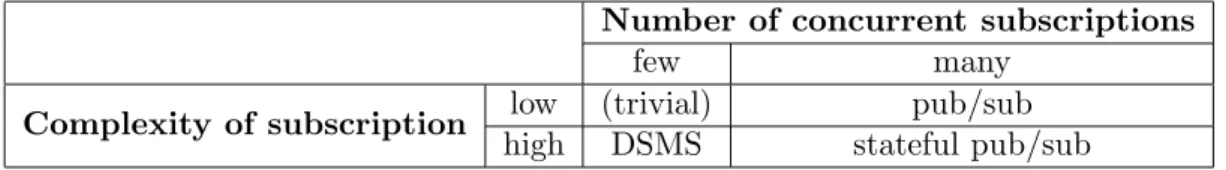
2.3. Stream processing 17 Number of concurrent subscriptions

few many

Complexity of subscription low (trivial) pub/sub high DSMS stateful pub/sub

Table 2.1: Trade-offs between pub/sub and DSMS (from Demers et al.)

streaming data such as sensor networks or stock exchanges. As an example, Cayuga can handle sequences of events such as the following subscribe query taken from Demers et al. “Notify me when the price of IBM is above $100, and the first MSFT price afterwards is below$25” ??. In this case the stream processor has to store state in order to evaluate the query.

The authors compare Cayuga to Data Stream Management Systems (DSMS), which offer query languages to the same effect, but fail to scale over a large number of subscriptions. The difference between a traditional DSMS such as STREAM and Cayuga is shown in Table 2.1 [20]. Cayuga, however, is still closely related to the database community. The query language called Cayuga Event Language (CEL) is similar to SQL [20]. Like STREAM, Cayuga works with event streams - temporally ordered sequences of tuples. However, instead of using a single timestamp, Cayuga uses a start and end timestamp during which the event was active. This gives a duration as well as a “detection time“ [13].

Cayuga includes unary relational algebra operators such as selection, projection and renaming. It supports union, but it excludes Cartesian products and window join. These unrestricted joins are less useful in a stream setting as they are not taking into account the timestamps of the events. Instead Cayuga offers a sequencing and aniteration operator.

• Sequencing operator(;θ) The sequencing operator is a forward-looking combining join

that processes the event stream in sequence and tries to satisfy the filter predicate θ. • Iteration operator(µξ,θ) The iteration operator allows more complex joins. Here ξ can

be any unary operator such as projection.

The implementation behind Cayuga is a single node system based on non-deterministic finite automata. The approach used to evaluate queries is very similar to the one used in regular expressions. CEL queries are compiled into state machines and then loaded into the query engine via an intermediate XML format [13]. Predicates are mapped to edges and events are affecting the state of the automaton. Like with regular expressions, an edge is only traversed if the incoming event satisfies the predicate. If no edges are traversed, the event cannot satisfy the query and is thus dropped.

Distributed Cayuga

Brenna et al. have developed a distributed version of Cayuga [13]. We will discuss two of the techniques they used -Row/Column scaling and Pipelining.

Row/Column scaling A simple technique to scale query processing in stateless systems is to spread the queries over n machines. This row is then replicated m times to form a n×m

matrix. Events now can be routed to any row. Usually the routing is done in a round-robin fashion, however. This causes a problem with stateful queries. In order to make use of states

(28)

we must route events to the same row. This is infeasible. Brenna et al. [13] propose two ways of partitioning the workload.

The first technique is to partition the input event stream into several substreams of related events. These substreams are then assigned to rows and processed individually. The partitioning itself can be expressed as a Cayuga query and done by a separate machine.

The second technique is to partition the query workload. Thus instead of sending substreams to the rows, each row receives a full copy of the input stream.

Pipelining Cayuga provides the possibility for queries to be split into sub-queries if the former can not be run on a single machine. The output of one subquery to another is controlled via a feature called re-subscription [13].

Evaluation Cayuga and the effort to run it over large distributed networks are two interesting approaches. In the single node implementation Cayuga with its very expressive CEL language makes a lot of sense. However, in the distributed case, the situation is more complicated. For our project we are planning to start with a single query which means that the ideas concerning row/column scaling are currently not applicable.

2.3.4 MapReduce Online

MapReduce Online enables ”MapReduce programs to be written for applications such as event monitoring and stream processing“; it has been proposed in a technical report by Condie et al. in 2009 [18]. In contrast to the original Google implementation of MapReduce [19], Condie et al. propose a pipelined version in which the intermediate data is not written to disk. The prototype for this concept is a modification of the Hadoop framework and calledHadoop Online Prototype

(HOP).

The first change the authors introduced into stock Hadoop is pipelining. Instead of writing data to disk, it is now delivered straight from the producers (map tasks) to consumers (reduce tasks) via TCP sockets. If a reduce task has not been scheduled yet, the data can be written to disk as in plain Hadoop. The number of connections is also bounded to prevent creating too many TCP connections. Combiners are facilitated by waiting for the map-side buffers to fill before they are sent to the reducers. This enables us to pre-process the data before it is sent to the reducers. The processed data is written to a spill file which is monitored by a separate thread. This thread transmits the data to the reducers. The spill files enable simple load balancing between the mappers and reducers as their size and number reflects the load difference in the system. If spill files grow, we can adaptively invoke a combiner function on the side of the mapper to even the load.

The Hadoop Online Prototype further allows for inter-job pipelining. It must be noted that it is impossible to overlap the previous reduce with the current map function as the former has to complete before the latter can start. However, pipelining reduces the necessity to store interme-diate result in stable storage which could be costly. Condie et al. have extended Hadoop to be able to insert jobs ”in order“. This helps to preserve dataflow dependencies. The introduction of pipelining into Hadoop makes the system ready for running streaming applications.

(29)

2.4. Load balancing 19 Evaluation The Hadoop Online Prototype is a very interesting approach for stream process-ing. The changes over ordinary MapReduce implementations are subtle but powerful. However, like all other technologies visited in this section, HOP does not automatically scale during run-time. The number of map and reduce tasks is fixed. This impairs the ability of the MapReduce implementation to cope with varying load. We have chosen to use Hadoop as a starting point to design a stream processor utilising the MapReduce paradigm.

2.4

Load balancing

Load balancing is an integral part of our system’s design. A single stream processing node should automatically move computation to the cloud when its own resources are not sufficient anymore. In this project we aim to do this in a way which avoids an increase in latency and gives a guarantee on QoS properties of the system. To find possible strategies to achieve this, we have studied several load balancing strategies for webservers. First there are client side policies in which the client decides which server to use. Client-side policies include NRT (network round-trip-time) and latency estimated from historical data [14]. Selection algorithms are also based on hop count or geographical distance. We are also interested in server side policies which use a load index to determine how to route requests. Both are applicable as we run the local stream processor and evaluate its load on the same machine. However, none of the research mentioned in this section is 100 percent applicable to our situation. We are not aware of a load-balancing solution that evaluates computational load at a single front-end node and moves the overhead into a scalable cluster.

2.4.1 Load-balancing in distributed web-servers

Cardellini et al. discussed the state of the art in locally distributed web-server systems [15]. While our load-balancing or load-sharing algorithm is located at layer 7 (i.e. application layer of the OSI model) this paper gives insights into routing at all layers. We are especially interested in the discussion of a proxy for routing the requests (TCP gateway) and the discussion about dispatching algorithms. In our use-case we are looking for a load sharing algorithm that smooths out transient peak overload. This algorithm must be dynamic as we require it to have information about the state of the system. Finally, we must decide between centralised and distributed algorithms. As we will do the load balancing on the single machine serving as a controller to the cloud computations and the initial worker node, we opt for a centralised algorithm here. As mentioned in the article, fundamental questions are which server load index to use, when to compute it and how this index is shared with the orchestrating server. Ferrari and Zhou found that load indices based on queue length perform better than load indices based on resource utilisation [23]. They define the load index as a positive integer variable. It is 0 if the resource is idle and increases with more load. We must further acknowledge that there is no general notion of load. For example the CPU might be idle in a heavily I/O bound process, while in other cases processes are competing for CPU time. To summarise, the following load indices are mentioned in Ferrari and Zhou [23].

• CPU queue length • CPU utilisation

• Normalised response time4 4

(30)

Evaluation Our load balancing exercise will mainly concentrate on the local node as for the cloud this should be done by the MapReduce framework. This means that we can easily calculate the normalised response time. If this time exceeds a certain threshold we can start moving computational load to the cloud. Queue length is also a good indicator of load. In the evaluation chapter of this report we shall look at both response time and queue length.

2.4.2 Locally aware request distribution

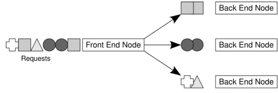
Pai et al. suggest a load balancing based on data locality [32]. In this system called LARD (locally aware content distribution), a single frontend receives the requests from clients. These requests are usually for static web content. This static content is stored on a number of back-end webservers. Once the first request for a particular resource comes in, the front-end examines it and routes it to the server with the least load. Any subsequent requests for this file are (if possible) routed to the same server. This makes sure that this back-end server can efficiently cache the data. Furthermore, it enables the design of a scalable storage system. We can spread the data over multiple back-end servers with little replication. Each request will be routed to a different server thus resulting in an efficient architecture. This works especially well for websites as http is a connectionless protocol and for every file, a new connection is opened.

Figure 2.2: Structure of LARD system

In order to implement the LARD system, the front-end server has to examine the incoming requests. In contrast to routing at OSI level 4, the front-end has to examine the request to know which backend-server should deal with the request [32]. Furthermore, the front-end needs to know about the individual loads at the backend. In their discussions, Pai et al. assume that the front-end and the network have no degrading effect on the performance of the overall system.

Evaluation LARD is only remotely applicable to our stream processing application. LARD is distributing the requests over servers in order to reduce cache misses. The only stable data in our system are the queries. The streaming data must not be stored but processed immediately. An additional complication is introduced by the fact that in our case the front-end takes part in the processing. This breaks with the assumption that the performance is independent of the front-end.

2.4.3 TCP Splicing

TCP slicing is a technique implemented in layer 7 switches to improve performance [17]. Like the LARD protocol above, layer 7 switches are able to do URL aware redirection of HTTP traffic. The benefits are the aforementioned cache hit rate and the ability reduce the need for replication in the backend. In this scheme, the switch acts as a proxy and redirects incoming

(31)

2.5. Summary 21 HTTP requests based on the URI in the GET request. Incoming requests are examined and and the switch queries the right backend server for the response.

While layer 4 switching is based on port and IP, layer 7 switches work at the application layer. As application data is only transferred once the connection has been established we cannot do URI aware routing without first establishing a connection between the client and the switch. This means that we need to establish two connections. The first connection is between the client and the switch. The second connection is between the switch and the backend server. The most common form of handling this problem is called TCP gateway. The TCP gateway solution simply forwards the packets from the backend over the switch at the application layer. However, this is unnecessary. Once we have established the connection between the client and the switch and located the right backend server, any subsequent reply from the backend can be forwarded over layer 4. This technique is called TCP splicing. Packets from the server to the switch are translated to look as if they had passed through the application layer in the TCP gateway protocol. As we do not have to examine the content but only to rewrite sequence number addresses, this is relatively simple and can be done with little to no overhead. TCP slicing is very effective for large files as the number of outgoing packets is much greater than the incoming requests. But even for data as small as 1Kb, significant performance benefits can be obtained [17].

Evaluation TCP slicing only concerns how the data is being handled by the switch. The actual load balancing is not affected. This technique is very interesting for us as we will need to redirect the output from the cloud to the clients. However, the response is likely to be shorter than the incoming data (as discussed above). Furthermore, we cannot afford to create too much overhead in the local server as we would like to use it for processing as well. An interesting case arises when the amount of work done in the cloud eclipses the work done locally by a few times. In this case, the local machine may become merely a coordinator and the TCP slicing solution viable.

2.5

Summary

In this chapter we have covered the design principles of the MapReduce framework. We have discussed the original paper by Google [19] and a streaming variant called HOP based on the Hadoop framework [18]. We will be using the MapReduce paradigm to design a scalable stream processor. The discussion on remote procedure calls (RPC) serves to give the necessary back-ground for the custom MapReduce prototype introduced in Chapter 4. The short introduction to Amazon’s EC2 should remind us of the ultimate goal which is to move the auxiliary stream processor to an IaaS provider. We have reviewed the current state of the art in stream processing and hinted why none of the existing systems are designed to be used on a cloud infrastructure. This chapter was concluded with an overview of some existing load balancing techniques and their limitations when applied to our specific situation. We are not aware of a load-balancing so-lution which supports a single-node stream processor through an auxiliary, scalable, cloud-based stream processor.

(32)

(33)

Chapter 3

Stream Processing With Hadoop

In this chapter we will discuss our efforts to extend the MapReduce paradigm to continuous queries. We will show the design and implementation process leading to a MapReduce stream processor which can be run on a cloud infrastructure. We will start by showing how we can extend Hadoop to accept a TCP stream as a data source. We will then discuss how the concept of jobs can be extended to continuous queries. This chapter will be concluded with a discussion on the architectural limitations of Hadoop as a stream processor. The evaluation of our results will follow in Chapter 6.

3.1

From batch to stream processing

We have chosen Hadoop as the basis for our streaming MapReduce as it has already been adopted in a range of industry projects [10] [25] [35]. The main advantage of this is that the acceptance of a streaming solution is likely to be greater with this already proved software. Hadoop is open-source software and therefore amenable for extensions and modifications.

The key to our evaluation of the MapReduce framework will be the guarantees given on latency and the capability to scale efficiently as the load is increased.

Hadoop is designed for batch-processing. A typical Hadoop job takes hours and is run on dozens of machines [19]. A query in a stream processing system must typically be executed in seconds or milliseconds. Therefore, some modifications are necessary to adopt Hadoop for stream processing. As discussed in the background section (see §2.2.3 and §2.3.4), we shall be using a modified version of Hadoop, the Hadoop Online Prototype [18] (HOP), for our experiments. There are two main tasks, we need to achieve before we can use Hadoop to process continuous data streams:

1. Network I/O Hadoop needs to be able to forgo the distributed file system and read its data straight from a network socket. Likewise, the output of the MapReduce operation has to be written to a socket for delivery to the client.

2. Persistent queries Hadoop is designed to accept one job per input directory. We can submit many jobs in succession, but there it is currently impossible to install a persistent query.

(34)

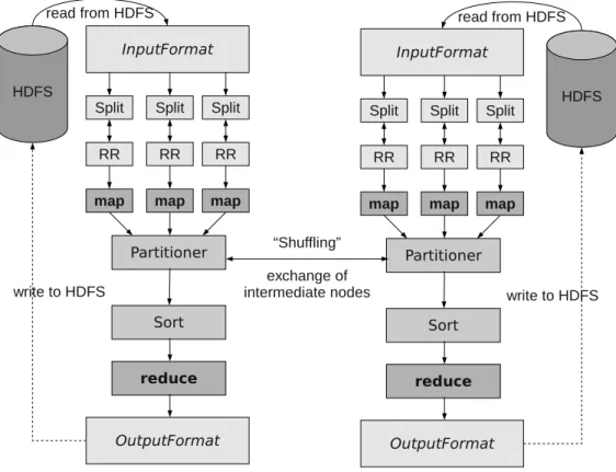
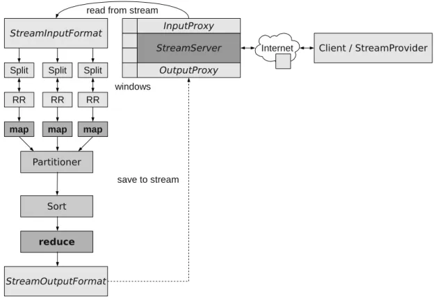
Figure 3.1: Hadoop dataflow on two nodes. InputFormat determines InputSplits and RecordReaders (RR). Map tasks get their data from the RRs and pass them to the Partitioner for grouping prior to the reduce stage. The reduced data is collected by RecordWriters as defined in the OutputFormat. Diagram adapted from http://developer.yahoo.com/hadoop/tutorial/module4.html

3.2

Network I/O

Traditional Hadoop approach

Hadoop relies heavily on its distributed file system to provide the data to mappers and reducers (Figure 3.1). Streaming applications could use the ZooKeeper [3] tools to control the distributed file system and monitor changes. We could simply write a server which uploads incoming data to the file system and a corresponding ZooKeeper task to act on any changes to the HDFS. With our low latency constraint, however, we cannot afford to store the window on the distributed file system data prior to processing. Use of the distributed file system would incur a significant overhead in processing and prevent us from being able to give any sort of latency guarantee. The distributed file system must be eliminated from the MapReduce cycle (Figure 3.1) in order to accomodate streaming queries.

Stream server

The first step in making the HDFS obsolete is to extend the Hadoop framework to obtain input splits from a network socket. The HOP implementation ensures that the intermediate data is only stored if really necessary. The output stream is written to a socket as well. All data is transient and the system completely stateless.

In order to implement the input and output streams, we need to introduce an additional stream server into the HOP framework (Figure 3.2). The StreamServer is invoked once and then handles

(35)

3.2. Network I/O 25

Figure 3.2: Hadoop dataflow with StreamServer component

the communication with the mappers and reducers. As the StreamServer and the MapReduce job do not know the size of the window in advance, this information is communicated as part of the control information of every window. This information can then be used with the split size to create input splits for the mapper processes. Once a query is invoked, the mappers block until data is available from the StreamServer. The result is then processed and handed over to the reducers. Once the reducers have finished, the information is relayed back to the StreamServer and communicated back to the invoker of the query.

3.2.1 Implementation of the changes

Listing 3.1 shows how the implementation of streaming queries has changed the way in which we have to write a Hadoop MapReduce job. The changes have necessitated the development of a new way of handling the input.

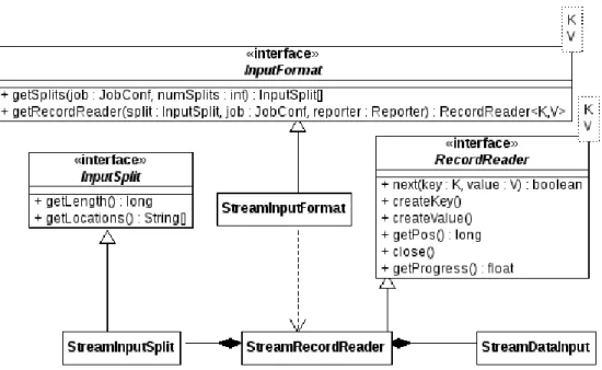
StreamInputFormat

Hadoop uses the JobConfclass to assert whichInputFormathas been chosen by the user (List-ing 3.3). The InputFormat class tells the Hadoop framework where to get the input splits from. In the original implementation this could be for example a file or folder on the distributed file system or a distributed database. The InputFormat class is generated on the fly by reflection from the JobClient. We therefore have to set its parameters using reflection, too. This can be achieved by using a static method as shown on line 8 in Listing 3.1. As the the given InputFor-mat classes do not contain provision for sockets, we have to create our own implementation. We have done so in the form of a newStreamInputFormatclass. Like the existing implementations, StreamInputFormat is a factory for the RecordReader class (“RR” in Figures 3.2 and 3.1). The

(36)

1 _{S t r e a m S e r v e r . s t a r t S e r v e r ( 5 0 0 0 2 ) ;}

2 _{// C r e a t e a new j o b / query c o n f i g u r a}