D
ynamic
L
inear
M
odels of
S
ensor
D
ata
Y
ingying
L
ai
Thesis submitted for the degree of
Doctor of Philosophy
School of Mathematics, Statistics&Physics Newcastle University
Newcastle upon Tyne United Kingdom
We develop a spatio-temporal model to analyse pairs of observations on temperature and humidity. The data consist of six months of observations at five locations collected from a sensor network deployed in North East England. The model for the temporal component takes the form of two coupled dynamic linear models (DLMs), specified marginally for temperature and conditionally for humidity given temperature. To account for dependence at nearby locations, the governing system equations include spatial effects, specified using a Gaussian process. To understand the stochastic nature of the data, we perform fully Bayesian estimation for the model parameters and check the model fit via posterior distributions. The intractability of the posterior distribution necessitates the use of computationally intensive methods such as Markov chain Monte Carlo (MCMC). The main disadvantage of MCMC is computational inefficiency when dealing with large datasets. Therefore, we exploit a class of sequential Monte Carlo (SMC) algorithms known as particle filters, which sequentially approximate the posterior through a series of reweighting and resampling steps. The tractability of the observed data likelihood under the DLM admits the implementation of an iterated batch importance sampling (IBIS) scheme, which additionally uses a resample-move step to circumvent the particle degeneracy problem. To alleviate the computational burden brought from the resample-move step of IBIS, we develop a novel online version of IBIS by modifying the resample-move step through approximating the posterior over an observation window whose pre-specified length trades offaccuracy and computational cost. Furthermore, performing the resampling step independently for batches of parameter samples allows a parallel implementation of the algorithm to be performed on a powerful multi-core high performance computing system. A comparison of observed measurements with their one-step and two-step forecast distributions shows that the model provides a good description of the underlying process and provides reasonable forecast accuracy.
I would like to express my sincere gratitude to my supervisors Prof Richard Boys and Dr Andrew Golightly for their guidance and encouragement. I would like to thank Prof Phil Taylor and the Newcastle Urban Observatory team for giving advice on data exploration. I would like to thank the School of Mathematics, Statistics and Physics for providing a pleasant environment, and the Faculty of Science, Agriculture and Engineering for funding this research. Finally, I would like to pass on my heartfelt appreciation to my families and friends for their selfless love and support.
Parts of this thesis have been published by the author:
• Lai, Y., Golightly, A. and Boys, R. J. (2018). Sequential Bayesian inference for spatio-temporal models of temperature and humidity data. Submitted.
Contents i List of Figures v List of Tables ix 1 Introduction 1 1.1 Thesis aims . . . 3 1.2 Outline of thesis . . . 4
2 Dynamic linear models 7 2.1 Introduction . . . 7 2.2 Seasonality . . . 10 2.2.1 Sinusoidal form DLM . . . 10 2.2.2 Fourier form DLM . . . 11 2.3 Bayesian inference . . . 13 2.3.1 Gibbs sampler . . . 14
2.3.2 Marginal Metropolis-Hastings (MH) algorithm . . . 19
2.3.3 MCMC diagnostics . . . 22
2.4 Posterior predictive checks . . . 24
2.4.1 Within-sample predictions . . . 25
2.4.2 Out-of-sample forecasts . . . 25
2.5 Simulation studies . . . 26
2.5.1 Local level model . . . 27
2.5.2 Sinusoidal form DLM . . . 32
3 Sequential Monte Carlo 39 3.1 Importance (re)sampling . . . 39
3.1.1 Importance sampling . . . 39
3.1.2 Importance resampling . . . 42
3.2 State filtering . . . 43
3.2.1 Sequential importance sampling (SIS) . . . 43
3.2.2 Bootstrap particle filter (BPF) . . . 45
3.2.3 Auxiliary particle filter (APF) . . . 47
3.3 State and parameter filtering . . . 49
3.3.1 Liu-West algorithm . . . 49
3.3.2 Storvik algorithm . . . 51
3.3.4 Iterated batch importance sampling (IBIS) . . . 54
3.3.5 Adaptive iterated batch importance sampling (aIBIS) . . . 57
3.3.6 Online IBIS . . . 58
4 Simulation studies 61 4.1 Comparison between fully adapted auxiliary particle filter and bootstrap particle filter . . . 61
4.2 Comparison between the Liu-West algorithm, the Storvik algorithm, particle learning, IBIS and aIBIS . . . 62
4.2.1 Local level model . . . 62
4.2.2 Sinusoidal form DLM . . . 67
5 Application to temperature and humidity data 75 5.1 Data collection . . . 75
5.2 Spatial DLMs . . . 76
5.2.1 Additional harmonics . . . 79
5.2.2 Spatial humidity DLM . . . 80
5.3 Inference . . . 81
5.4 Within-sample predictions and out-of-sample forecasts . . . 86
5.5 Model selection . . . 87
5.6 Parallel computing . . . 89
5.6.2 Parallelisation for resampling . . . 91
6 Results 97 6.1 Simulation study . . . 97
6.1.1 Comparison of full IBIS with serial resampling and parallelised local resampling . . . 98
6.1.2 Comparison of full IBIS and online IBIS . . . 98
6.2 Real data study . . . 98
6.2.1 Posterior output . . . 101
6.2.2 Predictive checks . . . 102
7 Conclusions 109
2.1 A variety of time series data. . . 8 2.2 Diagram of the state space model. . . 9 2.3 Trace plots of MCMC samples by using different uniform proposal distributions. 23 2.4 Left: simulated data; right: 10 marginal posterior realisations ofθ1:n. . . 28
2.5 Gibbs sampler diagnostics: (1). trace plot by taking burn-in=100 and thin-ning=20; (2). autocorrelation function for the thinned chain after the burn-in period; (3). the posterior distribution (black) and the prior distribution (grey). The true parameter values are indicated by the solid circles. . . 29 2.6 Mean and 95% credible interval of within-sample predictions against the data. . 30 2.7 Simulated data (-o-) with mean and 95% credible interval of the samples for
1-step, 2-step, 3-step and 4-step ahead forecast respectively (error bars). . . 30 2.8 MH diagnostics: (1). trace plot by taking burn-in=100 and thining=20; (2).
autocorrelation function for the thinned chain after the burn-in period; (3). the posterior distribution (black) and the prior distribution (grey). The true parameter values are indicated by the solid circles. . . 31 2.9 Comparison of the posterior distributions with the posterior means forV and
W through the Gibbs sampler (red) and the MH algorithm (blue). The true parameter values are indicated by the solid circles. . . 32 2.10 Left: simulated data; right: 10 marginal posterior realisations ofF1:nθ1:n. . . . 33
2.11 MCMC diagnostics (the Gibbs sampler): (1). trace plot by taking burn-in=100 and thining=20; (2). autocorrelation function for the thinned chain after the burn-in period; (3). the posterior distribution (black) and the prior distribution (grey). The true parameter values are indicated by the solid circles. . . 34 2.12 Mean and 95% credible interval of the differences between within-sample
pre-dictions and the data. . . 35 2.13 Simulated data (-o-) with mean and 95% credible interval of the samples for
1-step, 2-step, 3-step and 4-step ahead forecast respectively (error bars). . . 36 2.14 MCMC diagnostics (MH algorithm): 1. trace plot by thining=20; 2.
autocorre-lation function; 3. the posterior distribution (black) with the prior distribution (grey). The true parameter values are indicated by the solid circles. . . 37 2.15 Comparison of the posterior distributions with the posterior means forV and
W through the Gibbs sampler (red) and the MH algorithm (blue). The true parameter values are indicated by the solid circles. . . 38
3.1 Effective sample size. . . 45
4.1 Left plot: comparison of the posterior means of the state through FA-APF, BPF and MCMC over time. The true values of the state are indicated by the grey circles. Right plot: Comparison of the difference of posterior means with 95% credible intervals through FA-APF against MCMC and BPF against MCMC. . 63 4.2 Comparison of the posterior distribution ofθvia BPF (blue) and FA-APF (red)
and the MCMC output (histograms) att =1, . . . ,6 respectively. . . 64 4.3 Sequential posterior means with 95% credible intervals ofW andV over time,
calculated from the output of different SMC schemes. Top row: 3×10³particles; middle row: 5×10³particles; bottom row: 104particles. The true parameter values are indicated by the horizontal grey lines. . . 65
4.4 Comparison of the posterior distributions ofW andV through different SMC schemes given all the data with the MCMC output. Top row: 3×10³particles; middle row: 5×10³particles; bottom row: 104particles. The true parameter values are indicated by the solid circles. . . 66 4.5 Sequential posterior means with 95% credible intervals ofW1,W2,W3andV
through different SMC schemes using 3× 10³ particles over time. The true parameter values are indicated by the horizontal grey lines. . . 69 4.6 Sequential posterior means with 95% credible intervals ofW1,W2,W3andV
through different SMC schemes using 5× 10³ particles over time. The true parameter values are indicated by the horizontal grey lines. . . 69 4.7 Sequential posterior means with 95% credible intervals ofW1,W2,W3andV
through different SMC schemes using 104particles over time. The true parameter values are indicated by the horizontal grey lines. . . 70 4.8 Comparison of the posterior distributions ofW1,W2,W3andV through different
SMC schemes using 3×10³particles given all the data with the MCMC output. The true parameter values are indicated by the solid circles. . . 70 4.9 Comparison of the posterior distributions ofW1,W2,W3andV through different
SMC schemes using 5×10³particles given all the data with the MCMC output. The true parameter values are indicated by the solid circles. . . 71 4.10 Comparison of the posterior distributions ofW1,W2,W3andV through different
SMC schemes using 104particles given all the data with the MCMC output. The true parameter values are indicated by the solid circles. . . 71 4.11 Comparison of the posterior distributions ofW1,W2,W3andV through different
SMC schemes using 106particles given all the data with the MCMC output. The true parameter values are indicated by the solid circles. . . 72
5.1 Temperature and relative humidity data streams over time at each location. Periods of missingness are indicated just above the x-axis. . . 76 5.2 Scatter plots of temperature against relative humidity at each location. . . 77
5.3 Mean and 95% credible interval of the log Bayes factor comparing temperature sDLM against FDLM2 and FDLM1 against FDLM2, over time. . . 89 5.4 Mean and 95% credible interval of the log Bayes factor comparing humidity
sDLM against FDLM2 and FDLM1 against FDLM2, over time. . . 90 5.5 Left: work flow of a parallel program in a shared memory system; right: work
flow of a parallel program in a distributed memory system. . . 92 5.6 Actual speed-up by running parallel jobs through different numbers of cores in a
distributed memory system. . . 92
6.1 Marginal parameter posterior densities obtained from the output of the full IBIS scheme with a standard serial resampling step (histograms) and a parallelised local resampling step (red). The true parameter values are shown as solid circles. 99 6.2 Marginal parameter posterior densities obtained from the output of the full IBIS
scheme (histograms) and the online IBIS scheme with window widthsT = 100 (yellow),T = 300 (blue) and T = 500 (red). The true parameter values are shown as solid circles. . . 100 6.3 Map showing site locations and a 10 km radius from each site, within which the
spatial correlation for temperature is at least 0.76, and for humidity, is at least 0.64.103 6.4 Mean (——) and 95% credible interval for the difference between the
within-sample predictive and the observations, at each location (1–5) over time. The observation period is from 8th July 2017 04:00:00 to 29th July 2017 00:00:00. . 105 6.5 One-step ahead forecast mean (——) and 95% credible interval, at each location
(1–5) over time. The observations are indicated (•). The observation period is from 12th July 2017 08:00:00 to 14th July 2017 00:00:00. . . 106 6.6 Two-step ahead forecast mean (——) and 95% credible interval, at each location
(1–5) over time. The observations are indicated (•). The observation period is from 12th July 2017 08:00:00 to 14th July 2017 00:00:00. . . 107
2.1 ESS and ESS/sec for the parameters obtained by the Gibbs sampler and the MH algorithm. . . 31 2.2 ESS and ESS/sec for the parameters obtained by the Gibbs sampler and the MH
algorithm . . . 35
4.1 Comparison of the performance by LW, ST, PL, IBIS, aIBIS: CPU time (in seconds); bias (and RMSE in parentheses) of estimators of the posterior expecta-tionsED(W|x1:n),ED(V|x1:n) and standard deviationsSDL(W|x1:n),SDL(V|x1:n).
All results are obtained by averaging over 100 runs of each SMC scheme. . . . 68 4.2 CPU time (in seconds) by averaging over 100 runs of LW, ST, PL, IBIS and
aIBIS respectively. . . 72 4.3 Comparison of the performance by LW, ST, PL, IBIS, aIBIS: bias (and RMSE in
parentheses) of estimators of the posterior expectationsED(W1|x1:n),ED(W2|x1:n), D
E(W3|x1:n), ED(V|x1:n) and standard deviations SDL(W1|x1:n), SDL(W2|x1:n), L
SD(W3|x1:n), SD(VL |x1:n). All results are obtained by averaging over 100 runs
of each SMC scheme. . . 74
5.1 A summary of hourly average temperature and humidity data over the period 8th July 2017 to 31st December 2017 at five locations in North East England. . . . 77
6.1 Marginal parameter posterior medians and quantile-based 95% credible intervals obtained from the output of the online IBIS scheme. . . 102
Introduction
Recent advances in sensor technology and data management mean that it is now possible to reliably and affordably collect data with respect to city operations from different locations. The data collection is merely the starting point. The essential part is to be able to analyse this spatial data and build accurate models which can be used to understand the stochastic nature, interdependencies and correlations between these data sets. This will require the combination of stochastic modelling for the non-stationary dynamic processes, efficient inference procedures and advanced computing architectures for big data.
Climate is one of the most important environmental factors which plays a critical role in the global mission of urban sustainability. Consequently, it has attracted tremendous attention from academic scientists and industrial experts in recent decades. The literature contains several temporal models for temperature at a single location. For example, Campbell and Diebold (2005) proposed an autoregressive (AR) model with Fourier components to account for seasonality, a polynomial deterministic trend and a generalised autoregressive conditional heteroscedasticity (GARCH) error process. Further AR modelling approaches have been proposed by Härdle and Cabrera (2012), Benth et al. (2007) and Benth and Benth (2012), with the latter adopting a continuous-time approach. Generic approaches for spatial data sets at multiple locations are widely available (see e.g. Cressie (1993), Stein (1999), Ripley (2004), Diggle and Ribeiro (2004), Gelfand et al. (2010), Cressie and Wikle (2011) and Banerjee et al. (2014)). By considering multiple variables jointly, Hu et al. (2013, 2015) use a stochastic partial differential equation (SPDE) to model yearly temperature and humidity data at 120 locations and perform fully Bayesian inference via an integrated nested Laplace approximation (Rue et al., 2009). Gamerman and Migon (1993) gave a list of hierachical dynamic linear models (DLMs) used for the state
evolution, smoothing and filtering through the stages of the hierarchy. A Bayesian hierachical model with the state process regressing on a spatial effect was discussed by Nott et al. (2001). Shaddick and Wakefield (2002) proposed a multivariate hierachical DLM with space-time regression structures on pollutant data studies.
Fully Bayesian estimation of the model parameters is necessary for appropriate forecasts and the model fit can be checked through posterior predictive distributions, which allow for uncertainty within the stochastic model. Markov chain Monte Carlo (MCMC) methods are primarily used for the offline learning of static parameters. For a DLM, a forward filter backward sampler (FFBS) (Carter and Kohn, 1994; Frühwirth-Schnatter, 1994) coupled with a Gibbs sampling approach, provides a strategy for state and parameter learning. When interest lies solely in the marginal parameter posterior, a marginal Metropolis-Hasting scheme is possible. Computational efficiency is one of the main barriers for use of MCMC in an online phase, as a new Markov chain has to be simulated when a new observation becomes available.
Sequential Monte Carlo (SMC) methods known as particle filters (Del Moral, 1996; Liu and Chen, 1998) are a set of online posterior density estimation algorithms allowing the posterior density of the model parameters to be updated sequentially through a series of weighted samples (known in this context as particles). A basic SMC scheme consists of a sequence of propagation and reweighting steps, which can be performed independently for each particle. The methods therefore permit the use of parallel computing. The main issue of the SMC schemes is particle degeneracy. That is, as time increases, only a small number of particles remain with non-zero weights. This problem can be alleviated (somewhat) through the resampling step to remove the particles with small weights and multiply the particles with large weigths. The bootstrap particle filter (Gordon et al., 1993) and the auxiliary particle filter (Pitt and Shephard, 1999; Pitt et al., 2012) were proposed based on this idea. However these methods are only applicable for fixed and known parameter values. Liu and West (2001) introduced a kernel smoothing method which adds a jitter to each particle of static parameters before particle propagation to the next time point. Storvik (2002), Fearnhead (2002), Carvalho et al. (2010) and Lopes et al. (2011) also proposed the algorithms that exploit the tractability of the conditional parameter posterior. Unfortunately, these methods do not overcome the particle degeneracy issue entirely (Chopin et al., 2010; Rios and Lopes, 2013). The iterated batch importance sampling (IBIS) algorithm (Chopin, 2002; Chopin et al., 2013) uses a resample-move step (referred to here as the rejuvenation step) (Gilks and Berzuini, 2001) in order to circumvent the degeneracy problem, where resampled paticles are mutated through a MCMC kernel. Additionally, Fearnhead and Taylor (2013) discussed an extension of the IBIS scheme by allowing the scaling of the tuning parameter in the rejuvenation steps to be changed adaptively. Unfortunately, the computational cost of the rejuvenation step
increases as the IBIS algorithm runs, precluding its use in real time.
1.1
Thesis aims
In this thesis we focus on understanding the relationship between temperature and humidity, as these are two of the most important factors in driving other climate processes. Our primary objective is the development of dynamic models which can be used to understand the stochastic nature of temperature and humidity, as well as quantify their spatial dependencies. Moreover, in order to facilitate accurate forecasts in real time, we focus on developing algorithms which allow inferences to be made sequentially in real time.
The modelling approach developed here is motivated by the fine scale temporal nature of the available data. Dynamic linear models (DLMs) are widely used for system evolution learning and short term forecasting due to their simple and practical structures; see, for example, West and Harrison (1999) for an introduction. We exploit these properties here by specifying a marginal DLM for temperature and a conditional DLM for humidity given temperature. We account for spatial dependence at nearby locations by adding a spatial Gaussian process to the system equations, thereby smoothing spatial deviations from the underlying temporal model.
We perform fully Bayesian inference for the model parameters as each observation becomes available. Since the posterior distribution is intractable, we use sequential Monte Carlo (SMC) methods that approximate the posterior distribution at each time point through a set of weighted samples; see Fearnhead and Künsch (2018) for a recent review of SMC methods. Although the posterior is intractable, the observed data likelihood is available in closed form, allowing the implementation of the iterated batch importance sampling (IBIS) scheme of Chopin (2002) (see also Chopin et al. (2013)). Essentially, parameter particles are incrementally weighted by the observed data likelihood contribution of the currently available observation. Particle degeneracy is mitigated via a resample-move step (Gilks and Berzuini, 2001) which ‘moves’ each parameter particle through a Metropolis-Hastings kernel that leaves the target invariant. This step can be executed subject to the fulfilment of some degeneracy criterion e.g. small effective sample size. As noted above, the computational cost of the resample-move step increases as the algorithm includes more data, as it requires calculation of the observed data likelihood of all available information. To obtain a novel online IBIS algorithm, where the computational cost of assimilating a single observation is bounded, we modify the resample-move step by basing the observed data likelihood on an observation window whose length is a tuning parameter,
chosen to balance accuracy and computational efficiency. We use a simulation study to formulate practical advice on how to choose the size of this window.
Further computational savings can be made by employing a high performance computing system. Whilst the weighting and move steps can be performed independently for each particle, a basic implementation of the resampling step requires collective operations, such as adding up the particle weights. Our approach is to use a simple strategy which performs the resampling step independently for batches of parameter samples, thus allowing a fully parallel (per parameter batch) implementation of the algorithm to be performed. We quantify the effect of the approxi-mation induced by this approach using synthetic data. Finally, we apply the online IBIS scheme (with parallel implementation) to the observed dataset and examine the model reliability and forecast accuracy through comparison of observed measurements with their posterior predictive distribution.
1.2
Outline of thesis
The remainder of this thesis is organised as follows. In Chapter 2, we start with a review of the generic structure of the DLM. To account for the seasonality of the data, we introduce the sinusoidal form DLM and the Fourier form DLM that allows for multiple harmonics. A review of Markov chain Monte Carlo (MCMC) is given, with the details of the Gibbs sampler and the Metropolis-Hastings algorithm, followed by a brief discussion of some commonly used MCMC diagnostics. We give the within-sample predictive and out-of-sample forecast distributions for posterior predictive checks, which can be used to investigate the model fit. The chapter is concluded with comparison between the Gibbs sampler and the Metropolis-Hastings algorithm by fitting two DLMs to synthetic data.
In Chapter 3, we comprehensively review several state-of-the-art sequential Monte Carlo (SMC) methods. We initially introduce the fundamental concept of importance (re)sampling. Following that, we introduce sequential importance sampling (SIS), the bootstrap particle filter (BPF) and the auxiliary particle filter (APF), which are the sequential Bayesian schemes that can be applied to the problem of state filtering when the parameters are fixed and known. We also detail the schemes which are applicable to the presence of unknown parameters. They include the Liu-West algorithm, the Storvik algorithm and particle learning. The main issue of these schemes is particle degeneracy, where only a few particles with reasonable weights remain. We introduce the iterated batch importance sampling (IBIS) algorithm and its adaptive version
(aIBIS) that effectively circumvent particle degeneracy through the use of MCMC steps for particle rejuvenation. Finally, we provide a novel online version of IBIS which allows a bounded computational cost by running IBIS through separated observation windows.
A series of simulation studies for the comparison of different SMC schemes is presented in Chapter 4. We first compare the fully adapted APF and BPF by examining their posterior estimations of the state. Both schemes are implemented by fitting a simple DLM, the local level model to a synthetic data set. In the remainder of the chapter, we compare the Liu-West algorithm, the Storvik algorithm, particle learning, IBIS and aIBIS by fitting the local level model and the sinusoidal DLM respectively by assuming the model parameters are unknown. We find that the IBIS scheme offers the best performance, in terms of the accuracy of the posterior estimation and the computational cost.
In Chapter 5, the background of the real data collection is briefly introduced followed by a dis-cussion of the structures of the spatial DLMs for temperature and humidity. A general Bayesian inference approach for handling missing data is then outlined. We give details of the IBIS and online IBIS schemes for the spatial temperature DLM. We access the seasonality of temperature data by fitting the sinusoidal form DLM and the Fourier form DLMs separately, and compare these models by using the concept of the Bayes factor. Due to the independence of operations on each particle, we can take advantage of parallel computing technics for implementing the SMC schemes. The details of conducting the parallel jobs in shared and distributed memory system are discussed. Resampling steps preclude full parallelisation of SMC schemes. We therefore consider a local resampling method, where the particles are partitioned into disjoint subsets and the algorithm can be run for each subset independently.
The effect of local resampling on posterior accuracy is considered in Chapter 6, using synthetic data. Furthermore, online IBIS is compared with full IBIS, before the former is applied to the real data. Posterior predictive checks are presented.
Dynamic linear models
2.1
Introduction
A time series is a sequence of data points obtained at successive times. Due to advanced measurement techniques, time series data can be recorded on most aspects of our lives to capture the changes of nature and human behaviour, such as, weather, environment, energy consumption, stock price, etc; see Figure 2.1.
State space models, developed over last few decades, provide an abundant family of interpretable models for analysing time series data (see e.g. Harvey, 1989; West and Harrison, 1999). The hidden state is described by a latent component and is used to drive the stochastic process of a data stream. The state is typically unobserved, and evolves itself over time. Figure 2.2 shows the evolution of a simple univariate state space in which the continuous valued latent state process {θ0, θ1, . . . , θt−1, θt, . . .}evolves according to a first order Markov chain with transition density
π(θt|θt−1). The continuous-valued observation process{x1,x2, . . . ,xt−1,xt, . . .}is linked to the
latent state process at an arbitrary timet via the densityπ(xt|θt) and here it is assumed that the
observations are conditionally independent given the state process.
The dynamic linear model (DLM) is a special form of the state space model, with xt and θt
evolving according to a Gaussian distribution with linear dependence onθt−1. Due to its simple
0 200 400 600 10 15 20 25 t (hr) T emper ature ( ° C ) 0 50 100 150 200 250 5 10 15 20 25 30 t (hr) PM2.5 (µgm/3) 0 50 100 150 200 3000 3500 4000 t (0.5hr) Electr icity consumption (kW) 0 50 100 150 200 250 440 460 480 500 520 540 t (day) BP PLC stock (£)
Figure 2.1: A variety of time series data.
forecasting (West and Harrison, 1999). For the univariate case, a DLM may be written as Xt|θt ∼ N(Ftθt,Vt),
θt|θt−1∼ N(Gtθt−1,Wt)
whereFt,Gt,VtandWtare deterministic functions oftwhich may be constant in practice. Taking
Initialisation ? (?1 | ?0 ) ? = 1 ? = 2 ? = t-1
?
2 ? (?2 | ?1 ) ? (?t | ?t-1 ) ? (x1 | ?1 ) ? (x2 | ?2 ) ? (xt-1 | ?t-1 ) ? = t?
1?
0?
t-1?
tx
tx
t-1x
2x
1 ? (xt | ?t )Figure 2.2: Diagram of the state space model.
the DLM. In practice, the DLM is usually written as Xt = Ftθt+vt, vt indep ∼ N(0,Vt), θt =Gtθt−1+wt, wt indep ∼ N(0,Wt),
and these equations are known as the observation and system equation respectively. The observation errorvtand the system errorwt are white noise processes with the mean 0 and the
variancesVt andWt respectively.
The simplest univariate DLM is the locally constant DLM, also known as the local level model. This model has constant functions Ft =1,Gt =1 and variance componsentsVt = V,Wt = W.
The observation and system equations are Xt =θt+vt, vt indep ∼ N(0,V), (2.1) θt =θt−1+wt, wt indep ∼ N(0,W). (2.2) Hence, the state process evolves according to a simple random walk from which noisy obser-vations are taken. We will use this simple DLM to benchmark the performance of various competing inference schemes in Chapter 3.
For most practical applications, we will requireθt and Xtto be vectors. Extending the univariate
can be written generically as Xt =Ftθt+vt, vt indep ∼ N(0,Vt), (2.3) θt =Gtθt−1+wt, wt indep ∼ N(0,Wt) (2.4) where • Xtis anl×1 vector; • θtis an m×1 vector;
• Ft is thel×mobservation matrix; • Gtis them×msystem matrix; • Vt is thel ×l observation variance; • Wt is them×msystem variance.
Taking an initial distributionθ0∼ N(m0,C0), wherem0andC0are known hyper-parameters, completes specification of the multivariate DLM.
2.2
Seasonality
Cyclical behaviour or seasonality is a significant feature of many time series. Due to the periodic patten, it is natural to incorporate harmonic functions within the DLM. We consider two approaches for modelling seasonality: (i) a single harmonic in the observation equation and (ii) multiple harmonics in the state equation. For ease of notation in what follows, we consider a univariate observation process.
2.2.1
Sinusoidal form DLM
The observation equation is given by
Xt = Ftθt+vt, vt indep
whereθt = (θt,1, θt,2, θt,3)T and the observation matrix is given by
Ft = (cos(2πt/Px),sin(2πt/Px),1)
wherePx is the time corresponding to one complete period. The system equation takes the form
of (2.4) withGt =I3. For our applications, we takeVt =V and
Wt =W =diag(W1,W2,W3) = * . . . , W1 0 0 0 W2 0 0 0 W3 + / / / -.
We refer to this model as the sinusoidal form DLM. Note that the observation equation can be written as Xt =θ˜t,2cos 2πt Px −θ˜t,1 ! +θt,3+vt (2.6)
where the parameters in (2.5) and (2.6) are related using ˜ θt,1= q θ2 t,1+θt,22 , θ˜t,2= tan−1 θt,2 θt,1 ! . (2.7)
Hence, the sinusoidal form DLM captures seasonality (about a time varying basal levelθt,3) via
a sinusoid whose amplitude ˜θt,2and phase ˜θt,1vary according to two independent random walk
processes.
2.2.2
Fourier form DLM
When time series data exhibit more complex cyclical behaviour, additional harmonics may be used. The Fourier form DLM captures seasonality through linear combinations of periodic functions; see, for example, West and Harrison (1999) and Petris et al. (2009). By definition, a Fourier series is written as
X(t)= q X r=1 ( Arcos 2πrt Px ! +Brsin 2πrt Px ! ) + A0, (2.8)
that is, the summation ofqharmonic functions and a mean level term. To construct a Fourier form DLM, let the observation matrix be the 1×(2q+1) matrix partitioned as
so that the state vectorθt is of length 2q+1 and satisfies a system equation of the form (2.4)
with system matrix
Gt =G= diag(H1, . . . ,Hq,1). (2.10)
Here,Hr is a harmonic matrix given by
Hr =* , cos (2πr/Px) sin (2πr/Px) −sin (2πr/Px) cos (2πr/Px) + -, r =1, . . . ,q.
The Fourier form DLM is then given by (2.3) and (2.4) withFt andGtas in (2.9) and (2.10).
To understand the model structure, consider the simple case in which the system varianceW =0. Suppose thatθr 0= θr 0,1, θr0,2
forr = 1, . . . ,qso that the initial state is
θ0= θ10, . . . ,θq0, θ0,3T . The state att = 1 is θ1 =Gθ0= H1θ10, . . . ,Hqθ q 0, θ0,3 T . Substitutingθ1into the observation equation (2.3), we obtain
X1= q X r=1 θr 0,1cos 2πr Px ! +θr 0,2sin 2πr Px ! ! +θ0,3+v1.
Similarly, whent =2, by ignoringwtwe have that
θ2 =G2θ0 =
H12θ10, . . . ,Hq2θ0q, θ0,3 T
.
Due to the property of the harmonic matrix, that is (Hr)t = Htr, the state can be rewritten as
θ2 =
H2θ01, . . . ,H2qθ0q, θ0,3 T
. Therefore the observation equation att = 2 is
X2= q X r=1 θr 0,1cos 2πr Px ×2 ! +θr 0,2sin 2πr Px ×2 ! ! +θ0,3+v2,
Recursive use in this way of the property of the harmonic matrix gives
Xt = q X r=1 θr 0,1cos 2πrt Px ! +θr 0,2sin 2πrt Px ! ! +θ0,3+vt (2.11)
making clear the link between the Fourier form DLM and the Fourier series in (2.8). Note that when using theq =1 harmonic, the observation equation of the Fourier form DLM coincides with that of the sinusoidal form in (2.5) given by
Xt = θ0,1cos 2πt Px ! +θ0,2sin 2πt Px ! +θ0,3+vt.
However, in the case of non-zeroW, the error structures differ due to the use of the harmonic in the system equation for the Fourier form DLM, and in the observation equation for the sinusoidal form DLM.
Note that the number of harmonicsqmust be specified by the practitioner. Consequently, Fourier models withq= 1,2 are typically used in practice to limit the size of the parameter space (Petris et al., 2009).
2.3
Bayesian inference
Without loss of generality, consider equally spaced datax1:n= (x1, . . . ,xn)T to which we wish
to fit a DLM with latent statesθ0:n= (θ0, . . . , θn)T and static parametersφ= (φ1, . . . , φnpar)
T.
For ease of notation, we consider a univariate DLM with variance componentsVt = V and
Wt =W but note that extension of the methodology introduced here to multivariate DLMs with
arbitrary variance components is straightforward in principle. Upon ascribing a prior density π(φ) toφ, Bayesian inference may proceed via the joint posterior density
π(φ,θ0:n|x1:n) ∝ π(φ)π(θ0)π(θ1:n|φ)π(x1:n|θ1:n,φ) (2.12) where π(x1:n|θ1:n,φ)= n Y t=1 N(xt;Ftθt,V), and π(θ1:n|φ) = n Y t=1 N (θt;Gtθt−1,W).
Here N(·;m,V) denotes a normal density with mean (vector) m and variance (matrix)V. If primary interest lies solely in the static parameter vectorφthen we may consider the marginal posterior
whereπ(x1:n|φ) is the observed data likelihood given by π(x1:n|φ)= π(x1|φ) n Y t=2 π(xt|x1:t−1,φ). (2.14)
In practice, (2.12) and (2.13) are intractable, that is, closed form expressions for these densities cannot be obtained, necessitating the use of stochastic simulation algorithms such as Markov chain Monte Carlo (MCMC) and sequential Monte Carlo (SMC). In this chapter, we focus on the former, and provide two MCMC schemes for generating draws from (2.12) and (2.13). These are: the Gibbs sampler and (marginal) Metropolis-Hastings algorithm. For an in-depth discussion of MCMC, we refer the reader to Gamerman and Lopes (2006).
2.3.1
Gibbs sampler
The Gibbs sampler was first introduced by Geman and Geman (1984) for generating draws from Gibbs distributions, by alternately sampling from full conditional distributions. Gelfand and Smith (1990) were the first to point out to the wider statistics community that the approach could be used within the Bayesian paradigm, for scenarios where full conditional (posterior) distributions are available for sampling from. As with other MCMC schemes, the Gibbs sampler simulates from a Markov chain whose stationary distribution is the target (posterior) distribution of interest. The transition density is formed by the full conditional distributions.
Suppose now that interest lies in the marginal posteriorπ(φ|x1:n) given by (2.13). The Gibbs
sampler is given by Algorithm 1. The Gibbs sampler defines a homogeneous Markov chain with transition density π(φ|φ˜,x1:n)= npar Y i=1 π(φi|φ1, . . . , φi−1,φ˜i+1, . . . ,φ˜npar,x1:n), wherenparis the number of parameters.
Checking stationarity ofπ(φ|x1:n) can be achieved by showing that
π(φ|x1:n)=
Z
π(φ|φ˜,x1:n)π( ˜φ|x1:n)dφ˜ (2.15) using induction (Gamerman and Lopes, 2006). Formal convergence conditions can be found in Roberts and Smith (1994).
Algorithm 1Gibbs sampler
1. Initialise the chain withφ(0) = φ1(0), . . . , φ(0)npar
T
. For j =1, . . . ,N:
2. Obtain a new valueφ(j) fromφ(j−1) by continuous sampling from the full conditional distributions: • φ(j) 1 ∼π(φ1|φ (j−1) 2 , . . . , φ (j−1) npar ,x1:n) • φ(j) 2 ∼π(φ2|φ (j) 1 , φ (j−1) 3 , . . . , φ (j−1) npar ,x1:n) ... • φ(j) npar ∼ π(φnpar|φ (j) 1 , . . . , φ (j) npar−1,x1:n) 3. Set j := j +1. Return to step 2.
Upon discarding a number of sampled parameter values as “burn-in”, the remaining samples ofφ(j), j = 1, . . . ,N are treated as realisations from π(φ|x1:n). The Gibbs sampler provides
an efficient sampling mechanism provided that the full conditional distributionsπ(φi|φ−i,x1:n),
i = 1, . . . ,npar, have standard forms and are easy to sample from. However, for the DLMs
considered here, the parameter full conditionals are likely to be intractable, after marginalising out the dynamic states. Neverthless, it is often the case that conditional on the data and the dynamic states, parameter (component) full conditionals will be available for sampling from (for a suitable choice of prior). Moreover, the full conditional density of the dynamic states, π(θ1:n|φ,x1:n), is tractable. Consequently, the most natural implementation of the Gibbs sampler
targets the joint posteriorπ(φ,θ0:n|x1:n) by alternating between the following steps:
1. simulateθ0:nfromπ(θ0:n|φ,x1:n),
2. simulateφfromπ(φ|θ0:n,x1:n).
Performing step 1 is achieved using a forward filtering backward sampling algorithm, which we now describe in detail.
Forward filtering backward sampling (FFBS)
As above, for clarity of exposition we consider a univariate DLM with static variance components Vt =V andWt =W.
Consider the task of generatingθ0:n ∼ π(θ0:n|φ,x1:n). Note that the parameter vectorφremains fixed throughout this section and we therefore drop it from the notation where possible. A widely used method is known as forward filtering backward sampling (FFBS) (Carter and Kohn, 1994; Frühwirth-Schnatter, 1994). The basic idea is to first calculate the filtering distributions π(θt|x1:t) recursively, fort =1, . . . ,n. This is achieved using a forward filter also known as a
Kalman filter (Kalman, 1960). Upon reachingt = n, we may drawθnfrom the marginal posterior
π(θn|x1:n). The remaining dynamic states are then drawn in a backward sweep by exploiting the
decomposition π(θ0:n|x1:n) = π(θn|x1:n)π(θ0|θ1) n−1 Y t=1 π(θt|θt+1,x1:t). (2.16)
Note that due to the linear Gaussian structure of the DLM, both the filtering densitiesπ(θt|x1:t)
and the densitiesπ(θt|θt+1,x1:t) required in the backward sweep are Gaussian densities.
In detail, consider the forward filter and suppose that at timet−1, having observedx1:t−1, we
have the currently available posterior densityπ(θt−1|x1:t−1) = N(θt−1;mt−1,Ct−1). Using the
system equation (2.4) it should be clear that at timetthe prior density ofθt is
π(θt|x1:t−1) = N (θt;Gtmt−1, Rt)
where Rt =GtCt−1GTt +W. Then using the observation equation (2.3), we obtain the density of
the one step forecast as
π(xt|x1:t−1) = N
xt;FtGtmt−1, FtRtFTT +V
. (2.17)
Note that after observing xt, (2.17) gives the observed data likelihood increment. To update the
currently available posterior density, we first construct the joint distribution ofθt andXt. After
noting thatCov(θt,Xt) =Cov(θt,Ftθt+vt) = RtFtT, we obtain
* , θt Xt + x1:t−1∼ N * , Gtmt−1 FtGtmt−1 + -,* , Rt RtFtT FtRt FtRtFtT +V + - .
Conditioning on Xt = xt using standard multivariate normal results yields the updated posterior,
i.e. the required filtering distribution, as
where mt =Gtmt−1+RtFtT(FtRtFtT +V) −1(x t−FtGtmt−1), Ct = Rt−RtFtT(FtRtFtT +V) −1F tRt.
These steps can be executed fort = 1, . . . ,nto give the forward filter.
To obtain the constituent terms in (2.16) necessary for executing the backward sweep, note that the joint density ofθtandθt+1(givenx1:t) is
* , θt θt+1 + x1:t ∼ N * , mt Gt+1mt + -,* , Ct CtGTt+1 Gt+1Ct Gt+1CtGTt+1+W + - . Conditioning onθt+1gives π(θt|θt+1,x1:t) = N(θt;ht, Ht) where ht =mt+CtGTt+1(Gt+1CtGTt+1+W)−1(θt+1−Gt+1mt), Ht =Ct−CtGTt+1(Gt+1CtGTt+1+W)−1Gt+1Ct.
Algorithm 2 gives the full form of the FFBS scheme. Note the convention thatx1:0denotes the
empty set.
Example: local level model
Consider the local level model given by (2.1) and (2.2). Letφ= (V,W)T. The Gibbs sampler iterates over the following steps:
1. simulateθ0:nfromπ(θ0:n|φ,x1:n),
2. simulateφ1fromπ(φ1|φ2,θ0:n,x1:n) = π(φ1|θ0:n,x1:n),
Algorithm 2FFBS scheme Forward Filtering:
1. Initial distribution:θ0∼ N(m0,C0). Store the values ofm0andC0.
2. Fort =1, . . . ,n,
(a) Prior att. Using the system equation, we have that
θt|x1:t−1 ∼ N(Gtmt−1,GtCt−1GTt +W).
StoreRt = GtCt−1GTt +W.
(b) One step forecast. Using the observation equation, we have that Xt|x1:t−1∼ N
FtGtmt−1, FtRtFtT +V
. (2.18) Store the marginal likelihood contribution
π(xt|x1:t−1)= N xt;FtGtmt−1, FtRtFTT +V . (c) Posterior att: θt|x1:t ∼ N(mt, Ct), where mt =Gtmt−1+RtFtT(FtRtFtT +V) −1(x t−FtGtmt−1), Ct = Rt −RtFtT(FtRtFtT +V) −1 FtRt.
Store the values ofmt andCt.
Backward Sampling:
3. Sampleθn|x1:n∼ N(mn, Cn).
4. Fort =n−1, . . . ,0,
(a) Backward distribution: θt|θt+1,x1:t ∼ N(ht, Ht), where
ht = mt+CtGTt+1(Gt+1CtGTt+1+W)−1(θt+1−Gt+1mt),
Ht =Ct−CtGTt+1(Gt+1CtGTt+1+W)−1Gt+1Ct.
(b) Sampleθt|θt+1,x1:t ∼ N(ht, Ht).
Step 1 can be executed using the FFBS algorithm described in Algorithm 2. It now remains to derive full conditional distributions for the components ofφ. Specifying independent inverse gamma prior distributions for φ1 and φ2 permits a semi-conjugate analysis (that is, leads to
prior hyper-parametersαv, βv,αw, βw. The full conditional density ofφ1is π(φ1|φ2, θ0:n,x1:n) ∝ π(φ, θ0:n,x1:n) ∝ π(x1:n|θ1:n, φ1)π(θ1:n|φ2)π(θ0)π(φ) ∝ n Y t=1 π(xt|θt, φ1) | {z } observation equation n Y t=1 π(θt|θt−1, φ2) | {z } system equation π(θ0)π(φ1)π(φ2) ∝ π(φ1) n Y t=1 π(xt|θt, φ1) ∝ φ−(αv+ n 2)−1 1 exp* , − βv+ 1 2 n X t=1 (xt−θt)2 , φ1+ -Therefore, we obtain φ1|θ1:n,x1:n∼ IG* , αv+ n 2, βv + 1 2 n X t=1 (xt−θt)2+ -. Similar arguments lead to
φ2|θ0:n∼ IG* , αw+ n 2, βw+ 1 2 n X t=1 (θt−θt−1)2+ -.
2.3.2
Marginal Metropolis-Hastings (MH) algorithm
The Gibbs sampler provides a natural mechanism for sampling the joint posteriorπ(φ,θ0:n|x1:n),
provided that full conditional distributions are available for sampling from. Retaining only draws ofφgives a sample from the marginal parameter posteriorπ(φ|x1:n). However, in scenarios
where there is high dependence between the static parameters and dynamic states, it can be beneficial to directly target the marginal parameter posterior via MCMC. Since π(φ|x1:n) is
typically intractable, we consider a Metropolis-Hastings (MH) algorithm, which can be used for sampling a generic target density that is only known up to a multiplicative constant.
The Metropolis-Hastings algorithm, first introduced by Metropolis et al. (1953) and then gener-alised by Hastings (1970), constructs a reversible Markov chain whose stationary distribution is the target of interest. Two key ingredients are the proposal distribution with densityq(φ∗|φ) (which should be easy to sample from) and an acceptance probability A(φ∗|φ) whose form ensures that the target is stationary. Since we are targeting the marginal parameter posterior, we
Algorithm 3Marginal MH algortithm
1. Initialise the chain withφ(0). Set j = 1. 2. Proposeφ∗ ∼ q(φ∗|φ(j−1)).
3. Calculate the acceptance probabilityα(φ∗|φ(j−1)) of the proposed move, where α(φ∗|φ(j−1)) =min(1, A(φ∗|φ(j−1))) =min ( 1, π(φ∗|x1:n)q(φ(j−1)|φ∗) π(φ(j−1)|x 1:n)q(φ∗|φ(j−1)) ) . 4. With probabilityα(φ∗|φ(j−1)), setφ(j) = φ∗; otherwise setφ(j) = φ(j−1). 5. Set j := j+1. Return to step 2.
refer to the resulting MH algorithm as marginal Metropolis-Hastings; see Algorithm 3.
The MH algorithm defines a homogeneous Markov chain with transition density (assuming that the chain moves) given by
π(φ|φ˜,x1:n)= q(φ|φ˜)α(φ|φ˜).
It can then be easily checked that
π(φ|φ˜,x1:n)π( ˜φ|x1:n)= π( ˜φ|φ,x1:n)π(φ|x1:n)
which is known as the detailed balance equation. Integrating both sides of this equation with respect to ˜φgives equation (2.15) and so we see that the target π(φ|x1:n) is stationary. Formal convergence conditions can be found in Roberts and Smith (1994) and Tierney (1994).
Note that the acceptance probability simplifies to
A(φ∗|φ(j−1))= π(φ ∗)π (x1:n|φ∗)q(φ(j−1)|φ∗ ) π(φ(j−1))π(x 1:n|φ(j−1))q(φ∗|φ(j−1))
so that only the unnormalised posterior density is required. Furthermore, assuming that the components ofφare independenta priorigives
A(φ∗|φ(j−1)) = π(x1:n|φ ∗)q(φ(j−1)|φ∗)Qnpar i=1 π(φ ∗ i) π(x1:n|φ(j−1))q(φ∗|φ(j−1))Qnpar i=1 π(φ (j−1) i ) .
accep-tance probability becomes A(φ∗|φ(j−1)) = q(φ (j−1)|φ∗) q(φ∗|φ(j−1)) π(x1|φ∗) π(x1|φ(j−1)) n Y t=2 π(xt|x1:t−1,φ∗) π(xt|x1:t−1,φ(j−1)) npar Y i=1 π(φ∗ i) π(φ(j−1) i ) .
The constituent terms in (2.17) can be calculated using step 2(b) of the forward filter in Algo-rithm 2. Some common choices of proposal distribution are now discussed.
Choices of proposal distribution
Symmetric chains. If the proposal distribution is symmetric, then
q(φ(j−1)|φ∗)= q(φ∗|φ(j−1)).
In this case, the acceptance probability simplifies as A(φ∗|φ(j−1)) = π(φ ∗|x 1:n) π(φ(j−1)|x 1:n) (2.19) which only requires the (unnormalised) posterior distribution.
Random walk chains. A common choice of the proposal distribution is the random walk proposal, where
φ∗ = φ(j−1)+, ∼ N(0,Σ).
Using different values of the innovation varianceΣ will result in different mixing properties of the chain. IfΣis large, large jumps are proposed, but are likely to be rejected. Conversely, IfΣ
is small, small jumps are proposed that are likely to be accepted. This suggests an optimal tuning parameter that balances acceptance rate with exploration of the parameter space. Therefore, we usually multiply the innovation variance by a scaling parameter, sayγ, to optimise performance. A standard rule of thumb due to Roberts et al. (1997) and Roberts and Rosenthal (2001) is
Σ = 2.38
2
npar
V ar(φ|x1:n)
which leads to an acceptance rate of 0.234 for certain target distirbutions, as npar → ∞. In
practice, values of the acceptance rate between 0.1 and 0.4 usually give reasonable mixing, as measured by for example effective sample size; see Section 2.3.3 for further details. The
posterior varianceV ar(φ|x1:n) can be estimated via a pilot run of the MH scheme.
Note that if the innovation distribution is symmetric about zero, then we have a symmetric random walk chain with the acceptance probability defined by (2.19).
In many applications, parameter values must be strictly positive necessitating the use of a log normal random walk proposal, that is
logφ∗ = logφ(j−1)+˜, ˜∼ N(0,Σ˜)
where ˜Σis a scaled estimate of the posterior variance of logφ. The acceptance probability for the marginal MH algorithm can be written as
A(φ∗|φ(j−1)) = π(x1|φ ∗) π(x1|φ(j−1)) n Y t=2 π(xt|x1:t−1,φ∗) π(xt|x1:t−1,φ(j−1)) npar Y i=1 π(φ∗ i) π(φ(j−1) i ) npar Y i=1 φ∗ i φ(j−1) i .
Independence chains. As the name suggests, the proposed value is generated independently of the current position of the chain, so thatq(φ∗|φ(j−1)) = f(φ∗) for some density f(·). The acceptance probability becomes
A(φ∗|φ(j−1)) = π(φ ∗| x1:n) π(φ(j−1)|x 1:n) f(φ(j−1)) f(φ∗) .
When the prior is selected as the proposal distribution, the acceptance probability becomes A(φ∗|φ(j−1)) = π(x1:n|φ
∗)
π(x1:n|φ(j−1))
and hence only depends on the ratio of the likelihoods of the proposed value and the current value. Ideally, the acceptance probability should be as close to one as possible and so care must be taken when choosing the proposal density. For example, if the prior is used, significant difference in posterior and prior support can lead to an inefficient MH scheme.
2.3.3
MCMC diagnostics
The basic idea of MCMC methods is to construct a Markov chain whose equilibrium distribution is the target distribution. Therefore, investigating convergence of the Markov chain (or lack thereof) is essential when applying MCMC approaches. Informal visual checks are common
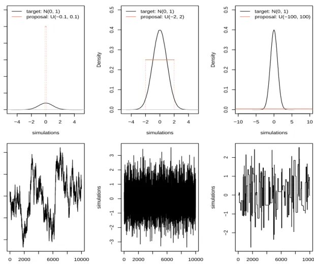
−4 −2 0 2 4 0 1 2 3 4 5 6 simulations Density target: N(0, 1) proposal: U(−0.1, 0.1) −4 −2 0 2 4 0.0 0.1 0.2 0.3 0.4 0.5 simulations Density target: N(0, 1) proposal: U(−2, 2) −10 −5 0 5 10 0.0 0.1 0.2 0.3 0.4 0.5 simulations Density target: N(0, 1) proposal: U(−100, 100) iterations sim ulations 0 2000 6000 10000 −2 −1 0 1 2 iterations sim ulations 0 2000 6000 10000 −3 −2 −1 0 1 2 3 iterations sim ulations 0 2000 6000 10000 −2 −1 0 1 2
Figure 2.3: Trace plots of MCMC samples by using different uniform proposal distributions.
place, and usually involve inspection of trace plots, which monitor the trajectory of MCMC samples. Applying the MH algorithm by taking the standard normal distribution N(0,1) as the target distribution and proposing the candidate samples through a random walk proposal with uniform innovations, Figure 2.3 shows the trace plots corresponding to different uniform innovations, i.e. sampled fromU(−0.1,0.1),U(−2,2) andU(−100,100) respectively, from left to right. When the random walk proposal hasU(−0.1,0.1), there is a high accepted rate and therefore the simulated samples are highly correlated. In the right column, the proposal has U(−100,100) which is too wide compared with the target distribution and causes most proposed samples being rejected. The proposal distributionU(−2,2) has the most comparable shape as the target distribution, hence the trace plot in the middle shows a good mixing.
As the initialisation of a chain is usually arbitrary and most likely not from a high density part of the stationary distribution, it is customary to remove a number of samples from the beginning of a chain. This number of iterations is the so called burn-in period (Gilks et al., 1996). In addition
to the visual examination of the trace plot, some formal methods on how to choose the length of burn-in period and assess convergence have been discussed by Heidelberger and Welch (1983), Geweke (1992), Gelman and Rubin (1992) and Raftery and Lewis (1996).
Successive MCMC draws are auto-correlated. If they exhibit a high degree of dependency, the chain will be slow to explore the parameter space. Moreover, posterior summaries based on such highly auto-correlated samples will generally have large variances. In order to get near independent MCMC samples, a simple method is to thin a chain by taking the value at everyith iterate. This procedure may also be important when long runs are required and memory storage is limited. However, to avoid information loss, we need to carefully select the frequency for thinning.
The autocorrelation function is used to quantify the dependency of samples at different lags. Assuming the chain is in equilibrium, let φ(j) be the value at jth iterate. The autocorrelation betweenφ(j) andφ(j+k) is
ρk =
E(φ(j)φ(j+k))−E(φ(j))E(φ(j+k)) V ar(φ(j)) .
For independent samples, the autocorrelation ρk is zero. For MCMC output, the (sample)
autocorrelation is 1 at k =0 and gradually decreases askincreases. A plot of the autocorrelation function can be useful in deciding an appropriate level of thinning. The autocorrelation function can further be used to determine the effective sample size (ESS) of a set of MCMC samples. The ESS of a run of length N can be roughly interpreted as the equivalent number of independent samples. It is given by
E SS = N
1+2P∞ k=1ρk
.
The estimation of the ESS requires estimating the spectral density at frequency zero and can be computed using theRpackage CODA (Plummer et al., 2006).
2.4
Posterior predictive checks
Posterior predictive checks are used to assess model validity by comparing suitably chosen predictive summaries to the observed data (Gelman and Hill, 2007). If the model is appropriate, there are not systematic discrepancies between the observed data and predictive summaries (Gelman et al., 2013). The predictive checks are usually conducted via calculation of the
within-sample predictive and out-of-sample forecast distributions.
2.4.1
Within-sample predictions
The within-sample predictive density is given by π( ˜x1:n|x1:n) =
Z Z
π( ˜x1:n|θ1:n,φ)π(θ1:n,φ|x1:n)dθ1:ndφ (2.20) where
π(θ1:n,φ|x1:n)= π(θ1:n|φ,x1:n)π(φ|x1:n). (2.21) Although the within-sample predictive density in (2.20) is intractable, draws fromπ(θ1:n,φ|x1:n) are readily available (via the Gibbs sampler, or marginal MH in conjunction with the backwards sampler) and thereforeπ( ˜x1:n|x1:n) can be sampled via Monte Carlo. Given draws (φ(j),θ1:n(j)),
j =1, . . . ,N from (2.21), we can simulate ˜
Xt(j)|θt(j),φ(j) ∼ N(Ftθt(j),V
(j)),
j = 1, . . . ,N, t =1, . . . ,n.
2.4.2
Out-of-sample forecasts
The system and observation forecast distributions can be obtained by exploiting the linear Gaussian structure of the DLM. The one-step ahead system forecast density is given by
π(θn+1|x1:n)= Z Z π(θn+1|θn,φ,x1:n)π(θn|φ,x1:n)π(φ|x1:n)dθndφ = Z π(θn+1|φ,x1:n)π(φ|x1:n)dφ where π(θn+1|φ,x1:n) = N θn+1;Gn+1mn,Gn+1CnGTn+1+W . Similarly, the one-step ahead observation forecast density is given by
π(xn+1|x1:n) = Z
where π(xn+1|φ,x1:n)= N xn+1;Fn+1Gn+1mn, Fn+1(Gn+1CnGTn+1+W)FnT+1+V . Hence, givenN posterior summaries (mn(j),C
(j)
n ),j = 1, . . . ,N fromπ(θn|φ,x1:n) andφ(j) from
π(φ|x1:n), the one-step ahead state and observation forecast distributions can be sampled via Monte Carlo, by drawing
θ(j) n+1|φ (j),x 1:n ∼ N Gn+1m(nj),Gn+1Cn(j)GTn+1+W (j) , Xn(+1j) |φ(j),x1:n ∼ N Fn+1Gn+1mn(j), Fn+1(Gn+1Cn(j)GTn+1+W (j))FT n+1+V (j) . For the general k-step ahead forecast, the above draws are replaced by
θ(j) n+k|φ,x1:n∼ N * , k Y i=1 Gn+i+ -m(nj), Rn(j)+k , x(nj)+k|φ(j),x1:n∼ N Fn+k* , k Y i=1 Gn+i+ -mn(j), Fn+kRn(j)+kFnT+k +V(j) , where Rn(+j)k =* , k Y i=1 Gn+i+ -Cn(j)* , k Y i=1 GTn+i+ -+ k−2 X j=0 * . , * . , j Y i=0 Gn+k−i+/ -W(j)* . , j Y i=0 GTn+k−i+ / -+ / -+W(j).
2.5
Simulation studies
In this section, we apply the Gibbs sampler and the marginal MH algorithm with a random walk proposal to synthetic data generated from the local level model and the sinusoidal form DLM considered in Sections 2.1 and 2.2.1.
2.5.1
Local level model
The simulated data stream consists ofn =200 observations with the error variancesV =2 and W = 1. Thus the local level model is
Xt = θt +vt, vt indep ∼ N(0,2), θt = θt−1+wt, wt indep ∼ N(0,1),
fort = 1, . . . ,n. The initial state is randomly drawn from N(10,9). The data are shown in Figure 2.4 (left panel). We takeV,W indep∼ IG(1,1) andθ0∼ N(10,16)a priorifor both of the
Gibbs sampler and the MH algorithm.
Results: Gibbs sampler
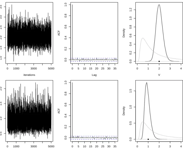
We consider the task of both state and parameter estimation. After discarding the first 100 itera-tions as burn-in, the Gibbs sampler was run for a further 105iterations, with the samples further thinned by taking every 20th iterate. Gibbs output diagnostics (trace plots and autocorrelation functions) can be found in Figure 2.5 alongside kernel desnity estimates of the marginal posterior densities ofV andW. The sampler mixes well with both traceplots suggesting convergence of the chain. Comparing the marginal posterior densities to the marginal prior densities shows that the data have been informative. Moreover, sampled values ofV andW are consistent with the true values that produced the data.
Realisations from the within-sample state predictive distribution are shown in Figure 2.4 and, unsurprisingly given the relatively small value of the observation variance, are consistent with the data. The within-sample observation predictive distribution is summarised in Figure 2.6 by the mean and 95% credible interval at each observation time. It is clear that there is no systematic difference between the predictive mean and the observations. Moreover, all observations lie within the 95% credible interval. Figure 2.7 shows the comparison between k-step forecasts (k =1,2,3,4) and the observations at each corresponding time points. The mean of the 1-step ahead forecast is very closed to the observed measurement att = 201. As the number of forecast steps gets larger, forecast uncertainty increases. We can see less accuracy for the 2-step, 3-step and 4-step ahead forecasts, although the observed measurements att = 202 andt = 203 still stay within the 95% credible intervals of the samples corresponding to 2-step and 3-step ahead forecasts.
0 50 100 150 200 5 10 15 20 t obser vation 0 50 100 150 200 5 10 15 20 t obser vation
Figure 2.4: Left: simulated data; right: 10 marginal posterior realisations ofθ1:n.
Results: MH algorithm
We now apply the MH algorithm to the same simulated data set. We chose the random walk proposal to generate proposed samples. First we conducted a pilot run with 2000 iterations and a small innovation variance for the random walk proposal: Σ = diag(0.01,0.01). In the full run, we used the same number of iterations, burn-in and thinning factor as for the Gibbs sampler for comparison. The innovation variance was calculated as the product of the scaling 2.382/2 and the variance of the samples from the pilot run. Figure 2.8 summarised the output
of the MH scheme. Again, the trace plots and autocorrelation functions suggest good mixing of the parameter chains. The posterior distributions of the parameters are both consistent with the true values that produced the data. Of course, both the marginal MH algorithm and Gibbs sampler target the same parameter posterior and we can see from Figure 2.9 that consistent output from both schemes is obtained. Forecasts are easily generated using the output of the marginal MH scheme (not shown). Within sample predictive summaries can be generated by repeatedly running the backward sampler for each sampled value of (V,W) from the parameter posterior (not shown).
The Gibbs sampler requires a full forward and backward sweep per iteration whereas the marginal MH scheme only requires the forward sweep. Consequently, the computational cost for running the Gibbs sampler is around 4 minutes ands running the MH algorithm takes 1.5 minutes. Plainly, when interest lies in the marginal parameter posterior, the marginal MH scheme provides an
iterations V 0 1000 3000 5000 1.0 1.5 2.0 2.5 3.0 3.5 0 5 10 15 20 25 30 35 0.0 0.2 0.4 0.6 0.8 1.0 Lag A CF 0 1 2 3 4 0.0 0.2 0.4 0.6 0.8 1.0 1.2 V Density iterations W 0 1000 3000 5000 0.5 1.0 1.5 2.0 0 5 10 15 20 25 30 35 0.0 0.2 0.4 0.6 0.8 1.0 Lag A CF 0 1 2 3 4 0.0 0.5 1.0 1.5 W Density
Figure 2.5: Gibbs sampler diagnostics: (1). trace plot by taking burn-in=100 and thinning=20; (2). autocorrelation function for the thinned chain after the burn-in period; (3). the posterior distribution (black) and the prior distribution (grey). The true parameter values are indicated by the solid circles.
efficient inference scheme. Moreover, draws from the marginal posterior of the dynamic states can be obtained post hoc, by appliying the backward sampler for parameter samples obtained from the (thinned) chain. Table 2.1 shows the numbers of ESS and ESS generated per second by the Gibbs sampler and the MH algorithm. Both schemes generated sufficient numbers of ESS, although the number of ESS for the parameter of system variance by the Gibbs sampler is relatively smaller than others. Because of less computational cost, the MH algorithm has a better performance than the Gibbs sampler in terms of ESS per second.
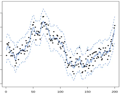
0 50 100 150 200 0 5 10 15 20 25 t obser vation
Figure 2.6: Mean and 95% credible interval of within-sample predictions against the data.
196 198 200 202 204 10 15 20 25 30 t 1−step ahead f orecast 196 198 200 202 204 10 15 20 25 30 t 2−step ahead f orecast 196 198 200 202 204 10 15 20 25 30 t 3−step ahead f orecast 196 198 200 202 204 10 15 20 25 30 t 4−step ahead f orecast
Figure 2.7: Simulated data (-o-) with mean and 95% credible interval of the samples for 1-step, 2-step, 3-step and 4-step ahead forecast respectively (error bars).
iterations V 0 1000 3000 5000 1.0 1.5 2.0 2.5 3.0 0 5 10 15 20 25 30 35 0.0 0.2 0.4 0.6 0.8 1.0 Lag A CF 0 1 2 3 4 0.0 0.2 0.4 0.6 0.8 1.0 1.2 V Density iterations W 0 1000 3000 5000 0.5 1.0 1.5 2.0 0 5 10 15 20 25 30 35 0.0 0.2 0.4 0.6 0.8 1.0 Lag A CF 0 1 2 3 4 0.0 0.5 1.0 1.5 W Density
Figure 2.8: MH diagnostics: (1). trace plot by taking burn-in=100 and thining=20; (2). autocorrelation function for the thinned chain after the burn-in period; (3). the posterior distribution (black) and the prior distribution (grey). The true parameter values are indicated by the solid circles.
Gibbs Sampler MH Algorithm
V W V W
ESS 16702 7642 13487 13517 ESS/sec 63 29 139 139
1.0 1.5 2.0 2.5 3.0 3.5 0.0 0.2 0.4 0.6 0.8 1.0 1.2 V Density 0.5 1.0 1.5 2.0 2.5 0.0 0.5 1.0 1.5 W Density
Figure 2.9: Comparison of the posterior distributions with the posterior means forV andW through the Gibbs sampler (red) and the MH algorithm (blue). The true parameter values are indicated by the solid circles.
2.5.2
Sinusoidal form DLM
In this example, we generatedn= 200 synthetic observations from the sinusoidal form DLM with time units in hours. We took the initial state vector to beθ0= (10,0,0) and the error variances
V =2 andW = diag(W1,W2,W3)= 2I3. The model then takes the form, fort =1, . . . ,n
Xt =Ftθt+vt, vt indep ∼ N(0, 2), θt =θt−1+wt, wt indep ∼ N(0, 2I3).
whereFt = (cos(πt/12),sin(πt/12), 1). We takeV,W1,W2,W3 indep
∼ IG(1,1) a priori. The data are shown in Figure 2.10 (left panel).
Results: Gibbs sampler
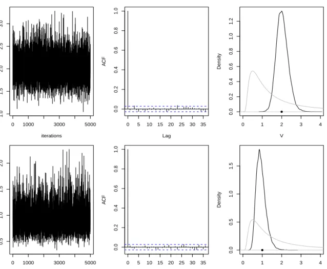
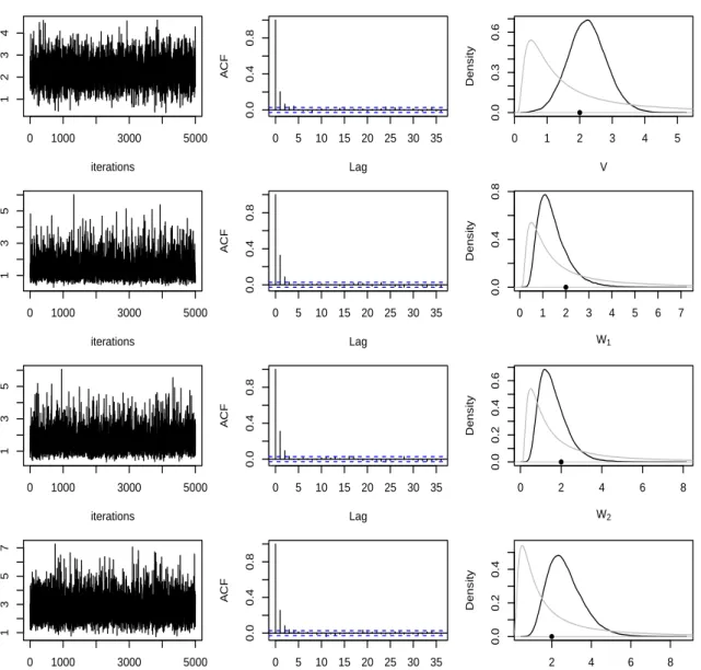
We ran the Gibbs sampler for 105 iterations, after discarding the first 100 values as burn-in. The output was then thinned by a factor of 20 to give 5000 values as the main monitoring run. Figure 2.11 summarises the output of the Gibbs sampler. All traceplots and autocorrelation functions suggest reasonable mixing. The marginal parameter posteriors are consistent with the
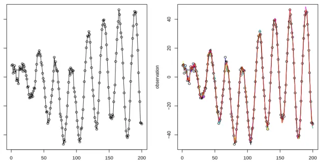
0 50 100 150 200 −40 −20 0 20 40 t obser vation 0 50 100 150 200 −40 −20 0 20 40 t obser vation
Figure 2.10: Left: simulated data; right: 10 marginal posterior realisations ofF1:nθ1:n.
true values that produced the data.
Realisations from the within-sample state predictive distribution are shown in Figure 2.4. Fig-ure 2.10 shows 10 realisations of Ftθt (right panel) which are broadly consistent with the
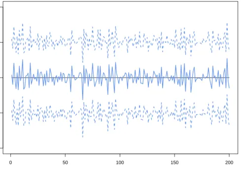
observations. In order to see any potential discrepancies between the within-sample observation predictions and the data more clearly, Figure 2.12 shows the mean and 95% credible interval of the difference between the samples generated from the within-sample predictive and the observation at each time point. Not surprisingly, this difference is plausibly zero at all time points.
Finally, Figure 2.13 shows k-step ahead forecasts (k = 1,2,3,4) against the corresponding observations. It is clear to that the forecast distributions are consistent with the observations, although the uncertainty increases as the number of forecast steps increases.
Results: MH algorithm
In the MH algorithm, we again chose the random walk proposal to generate proposed samples. A pilot run was conducted with 5000 iterations and a small innovation variance for the random walk proposal: Σ =diag(0.01,0.01,0.01,0.01). In the full run, we ran the marginal MH scheme with the same burn-in period, thinning frequency and total number of iterations as for the Gibbs sampler. We constructed the innovation variance by multiplying the scaling 2.382/4 with the
iterations V 0 1000 3000 5000 1 2 3 4 0 5 10 15 20 25 30 35 0.0 0.4 0.8 Lag A CF 0 1 2 3 4 5 0.0 0.3 0.6 V Density iterations W 1 0 1000 3000 5000 1 3 5 0 5 10 15 20 25 30 35 0.0 0.4 0.8 Lag A CF 0 1 2 3 4 5 6 7 0.0 0.4 0.8 W1 Density iterations W 2 0 1000 3000 5000 1 3 5 0 5 10 15 20 25 30 35 0.0 0.4 0.8 Lag A CF 0 2 4 6 8 0.0 0.2 0.4 0.6 W2 Density iterations W 3 0 1000 3000 5000 1 3 5 7 0 5 10 15 20 25 30 35 0.0 0.4 0.8 Lag A CF 2 4 6 8 0.0 0.2 0.4 W3 Density
Figure 2.11: MCMC diagnostics (the Gibbs sampler): (1). trace plot by taking burn-in=100 and thining=20; (2). autocorrelation function for the thinned chain after the burn-in period; (3). the posterior distribution (black) and the prior distribution (grey). The true parameter values are indicated by the solid circles.
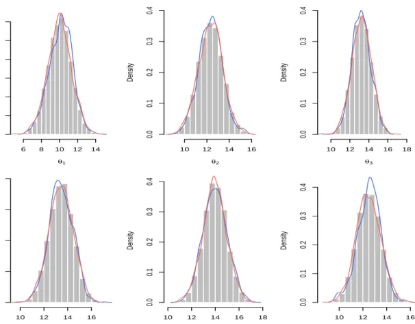
variance of the samples from the pilot run. Figure 2.14 summarises the MH output for each parameter chain. The traceplots and autocorrelation plots suggest convergence. The marginal posterior distributions are consistent with the true values and are also consistent with those obtained from the Gibbs sampler (see Figure 2.15). Similar results of within-sample predictions and out-of-sample forecasts are obtained for the MH scheme (not shown) as found in the previous section.
0 50 100 150 200 −10 −5 0 5 10 t prediction − obser v ation
Figure 2.12: Mean and 95% credible interval of the differences between within-sample predictions and the data.
Gibbs Sampler MH Algorithm
V W1 W2 W3 V W1 W2 W3
ESS 4214 2668 3061 3218 7230 5479 8408 6590 ESS/sec 2 1 2 2 24 18 28 22
Table 2.2: ESS and ESS/sec for the parameters obtained by the Gibbs sampler and the MH algorithm
respectively. The relative computational cost (for Gibbs:MH) increases from 2.7:1 for the local level model to 6.4:1 for the sinusoidal DLM. This is expected, since for the sinusoidal DLM, the backward sweep requires matrix operations (as opposed to scalar operations for the local level model). Table 2.2 shows the numbers of ESS and ESS generated per second by the Gibbs sampler and the MH algorithm. Unsurprisingly the MH algorithm presents a much better performance than the Gibbs sampler in terms of efficiency.
196 198 200 202 204 −40 −20 0 10 20 t 1−step ahead f orecast 196 198 200 202 204 −40 −20 0 10 20 t 2−step ahead f orecast 196 198 200 202 204 −40 −20 0 10 20 t 3−step ahead f orecast 196 198 200 202 204 −40 −20 0 10 20 t 4−step ahead f orecast
Figure 2.13: Simulated data (-o-) with mean and 95% credible interval of the samples for 1-step, 2-step, 3-step and 4-step ahead forecast respectively (error bars).
iterations V 0 1000 3000 5000 1 2 3 4 5 0 5 10 15 20 25 30 35 0.0 0.4 0.8 Lag A CF 0 1 2 3 4 5 0.0 0.2 0.4 0.6 V Density iterations W 1 0 1000 3000 5000 1 3 5 0 5 10 15 20 25 30 35 0.0 0.4 0.8 Lag A CF 0 1 2 3 4 5 6 7 0.0 0.4 0.8 W1 Density iterations W 2 0 1000 3000 5000 0 2 4 6 0 5 10 15 20 25 30 35 0.0 0.4 0.8 Lag A CF 0 1 2 3 4 5 6 7 0.0 0.3 0.6 W2 Density iterations W 3 0 1000 3000 5000 1 3 5 7 0 5 10 15 20 25 30 35 0.0 0.4 0.8 Lag A CF 0 2 4 6 8 10 0.0 0.2 0.4 W3 Density
Figure 2.14: MCMC diagnostics (MH algorithm): 1. trace plot by thining=20; 2. autocorrelation function; 3. the posterior distribution (black) with the prior distribution (grey). The true parameter values are indicated by the solid circles.