Sufficient information in structural VARs

RECent: c/o Dipartimento di Economia Politica, Viale Berengario 51, I-41100 Modena, ITALY

WORKING PAPER SERIES

Sufficient Information

in Structural VARs

Mario Forni and Luca

G

ambetti

Working Paper 62

June 2011

Sufficient Information in Structural VARs

∗

Mario Forni†

Universit`a di Modena e Reggio Emilia CEPR and RECent

Luca Gambetti‡

Universitat Autonoma de Barcelona June 6, 2011

Abstract

We derive necessary and sufficient conditions under which a set of variables is information-ally sufficient, i.e. contains enough information to estimate the structural shocks with a VAR model. Based on such conditions, we provide a procedure to test for informational sufficiency. If sufficiency is rejected, we propose a strategy to amend the VAR. Our method can be applied to FAVAR models and can be used to determine how many factors to include in such models. We apply our procedure to a VAR including TFP, unemployment and per-capita hours worked. We find that the three variables are not informationally sufficient. When adding missing infor-mation, the effects of technology shocks change dramatically.

JEL classification: C32, E32, E62.

Keywords: Structural VAR, non-fundamentalness, information, FAVAR models, technology shocks.

∗

We thank Fabio Canova, Marco Lippi and Luca Sala for helpful discussion. †

Financial support from Fondazione Cassa di Risparmio di Modena is gratefully acknowledged. Contact: Dipartimento di Economia Politica, via Berengario 51, 41100, Modena, Italy. Tel. +39 0592056851; e-mail: [email protected]

‡

The financial support from the Spanish Ministry of Science and Innovation through grant ECO2009-09847 and the Barcelona Graduate School Research Network is gratefully acknowledged. Contact: Office B3.1130 Departament d’Economia i Historia Economica, Edifici B, Universitat Autonoma de Barcelona, Bellaterra 08193, Barcelona, Spain. Tel (+34) 935814569; e-mail: [email protected]

1

Introduction

Since Sims (1980)’s seminal paper, Structural Vector Autoregression (SVAR) models have become extremely popular for structural and policy analysis. The idea behind these models is that structural economic shocks can be found as linear combinations of the residuals of the linear projection of a vector of variables onto their past values, i.e. are innovations with respect to the econometrician’s information set. Therefore, an obvious requirement for the analysis to be meaningful is that the variables used in the VAR convey all of the relevant information. Suchinformational sufficiencyis implicitly assumed in any VAR application.

But is this assumption always sensible? Unfortunately the answer is no. The basic problem is that, while agents typically have access to rich information, VAR techniques allow to handle a limited number of variables. If the econometrician’s information set does not span that of the agents the structural shocks are non-fundamental and cannot be obtained from a VAR (Hansen and Sargent, 1991, Lippi and Reichlin, 1993, 1994, Chari, Kehoe and Mcgrattan, 2008). Fernandez-Villaverde, Rubio-Ramirez, Sargent and Watson (2007) shows theoretical cases in which VAR techniques fail. Fiscal fore-sight and news shocks are two important examples (Leeper, Walker and Yang, 2008, Yang, 2008, Forni and Gambetti, 2010, Forni, Gambetti and Sala, 2010, Gambetti, 2010).

At now there is no generally accepted and systematic way to verify whether a spe-cific VAR suffers from this informational problem. In this paper we provide a testing procedure which is relatively easy to implement and valid under fairly general condi-tions. Moreover, we also we propose a strategy to amend the VAR when informational sufficiency is rejected.

Our main theoretical result is a necessary and sufficient condition for informational sufficiency, which is derived under the assumption that the economy admits a state space representation. Such condition is that there are no state variables that Granger cause the variables included in the VAR. The intuition is that the state variables convey all of the relevant information; therefore, if they do not help to predict a vector, such vector must contain the same information.

Based on this result, we suggest the following procedure. First, estimate the space spanned by the state variables of the economy by using the principal components of a large dataset, containing all available macroeconomic information. Second, test whether the estimated principal components Granger cause the variables included in the VAR. The variables are informationally sufficient if and only if the null hypothesis of no Granger causality is not rejected.

If a set of variables is not sufficient, we propose to estimate either a factor model, or a Factor Augmented VAR model (FAVAR), where the original set of variables is

enlarged with the principal components above. Our test can be applied recursively to the FAVAR in order to determine how many factors to retain. The number of factors is the minimum number such that the extended vector is informationally sufficient. To our knowledge, this is the first method suitable for FAVAR models.

As an additional result, we show that, even if the VAR is not informational sufficient to recover all of the structural shocks, still a single shock of interest can be correctly identified and estimated. In order for this to be the case, a necessary condition is that the shock must be orthogonal to the past of the state variables. This result can be used to test for structuralness of a shock as follows. First, identify and estimate the shock. Then test for orthogonality between this shock and the lags of the principal components. If the null of orthogonality is rejected, then the shock obtained from the VAR cannot be structural.

As an application we study technology shocks in the US. We test whether a small-scale VAR model, such as those typically used to study the effects of technology shocks, is informationally sufficient. Specifically, we use a VAR with total factor productivity, the unemployment rate and per-capita hours worked. We find that these three vari-ables are Granger caused by the first two principal components of a large dataset of US macrcoeconomic variables. Therefore we add such principal components to the VAR and show that the remaining principal components do not Granger cause the factor augmented VAR, meaning that the information conveyed in the FAVAR is sufficient. Finally, we identify the technology shock as the only one driving total factor produc-tivity in the long run, in both the original and the augmented VAR. Differences in the results in the two models are dramatic. While in the original VAR technology shocks increase hours and reduce unemployment, in the augmented VAR results are reversed: hours reduce and unemployment increases. Consistently with the test outcome, adding further factors does not change results any more. In the augmented model, investment and GDP react very sluggishly to the shock, prices fall and the real wage increases. Overall the result are hard to reconcile with the view that technology shocks are an important source of business cycle fluctuations.

The remainder of the paper is organized as follows. Section 2 presents theoretical results, as well as our proposed testing procedures. Section 3 discusses the application. Section 4 concludes. Appendix A reports the proofs. Appendix B reports information about the data used in the empirical application.

2

Theory

2.1 The macroeconomy

Assumption 1(MA representation). Then-dimensional vectorxtof stationary macroe-conomic time series satisfies

xt=F(L)ut, (1)

where ut is a q-dimensional, orthonormal white noise vector of structural macroeco-nomic shocks and F(L) is an n×q matrix of impulse response functions, i.e. square-summable linear filters in the non-negative powers of the lag operator L, such that

rank (F(z)) =q for some complex number z.

Representation (1) can be thought of as the representation of a macroeconomic equilibrium. Consider for instance the state-space representation studied in Fernandez-Villaverdeet al. (2007), i.e.

st = Ast−1+But (2)

xt = Cst−1+Dut (3)

where st is an r-dimensional vector of stationary “state” variables, q ≤r ≤n, A, B,

C and Dare conformable matrices of parameters, B has a left inverse B−1 such that B−1B =Iq. Pre-multiplying (2) byB−1 we getut=B−1(I−AL)st. Substituting this into (3) and rearranging gives

xt= DB−1+ (C−DB−1A)L

st. (4)

Stationarity of st ensures invertibility of (2), so that st = (I −AL)−1But. Combining this with (4) we get the MA representation

xt= DB−1+ (C−DB−1A)L

(I−AL)−1But, (5)

which is a special case of (1).

The assumption on the rank ofF(L) ensures that the representation is not redun-dant in the sense that there are no representations with a smaller number of shocks.

2.2 Sufficient information

Let us now define the information sets of the econometrician and the VAR, and the concept of sufficient information.

To begin, we assume that the SVAR econometrician observesxt, possibly with error. Allowing for a measurement error (which can be zero), besides being an interesting generalizationper se, will enable us to establish a link between the VAR model and the factor model introduced below, and extend our results to FAVAR models. Precisely:

Assumption 2. (Econometrician’s information set) The econometrician information set X_t∗ is given by the closed linear space spanned by present and past values of the

variables in x∗_t (in symbolsX_t∗ = span(x∗_1t, . . . , x∗_nt)), where

x∗_t =xt+ξt=F(L)ut+ξt, (6)

ξt being a (possibly zero) vector of measurement errors, orthogonal to ujt−k, j = 1, . . . , q, any k, and ξt−k, k >0.

In practice the number of observable variablesnis very large, so that the econome-trician needs to reduce it in order to estimate a VAR. The VAR information set is then spanned by ans-dimensional sub-vector ofx∗_t, or more, generally, ans-dimensional lin-ear combination ofx∗_t, say z_t∗ =W x∗_t (withs not necessarily equal to q). Considering also linear combinations will enable us to apply our results to the principal components of the variables and therefore to the FAVAR model.

Assumption 3 (VAR information set). The information set of the VAR is Z∗ t = span(z_1t∗_−k, . . . , z_st∗_−k, k≥0), where z_t∗ =W x∗_t, W being s×n.

Now, consider the theoretical projection equation ofz_t∗ on its past history, i.e.

z_t∗=P(z_t∗|Z_t∗₋₁) +t. (7)

The SVAR methodology consists in (a) estimating a VAR to gett; (b) attempting to get the structural shocks as linear combinations of the estimated entries oft. Hence a key property ofz_t∗ and the related information set is that the entries of t span the structural shocks, i.e. the information in the history ofz_t∗ is sufficient to estimate the shocks. We call such property “sufficient information”.

Definition 1(Sufficient information). We say that z_t∗ and the related information set

Z_t∗ contain “sufficient information” if and only if there exist a matrix M such that

ut=M t.

It is important to stress that sufficiency, defined in this way, is related only to the variables inz_t∗ and has nothing to do with the choice of a proper identification scheme. The correct identification ofM is a further problem, which in general does make sense only if sufficiency holds true.

2.3 The relation with fundamentalness

Informational sufficiency is closely related to “fundamentalness”. In this section we clarify the relation between the two concepts.1

From (6) and the definition of z_t∗ we get

z_t∗ =W F(L)ut+W ξt=zt+W ξt. (8)

1

Some important references about fundamentalness are Hansen and Sargent (1991), Lippi and Re-ichlin (1993, 1994), Chari, Kehoe and McGrattan (2008), Fernandez-Villaverdeet al. (2007).

Definition 2 (Fundamentalness). We say that ut is fundamental for wt = Hxt, and the MA representation wt = HF(L)ut is fundamental, if and only if ut ∈ Wt = span(w1t−k, . . . , wmt−k, k≥0)(i.e. Ut= span(u1t−k, . . . , uqt−k, k≥0) =Wt).

The following proposition formally establishes the relation between fundamentalnes and sufficiency.

Proposition 1. The information in z_t∗ is sufficient if and only if there is a matrix R

such that (a) z˜t=Rz∗t =Rzt and (b)ut is fundamental forz˜t.

For the proof see Appendix A. Proposition 1 says that, for z_t∗ being sufficient, there must be a linear transformation of z_t∗ which is free of measurement errors and have a fundamental representation in the structural shocks. Therefore, informational sufficiency is almost equivalent to fundamentalness plus absence of errors. If errors are small, informational sufficiency and fundamentalness essentially coincide; if, on the contrary, a VAR includes variables with large errors, information may be insufficient even if fundamentalness ofzt is met.

To conclude this subsection, let us observe that, in the particular case ofF(L) being a matrix of rational functions, fundamentalness ofutforwt, along with fundamentalness of the associated MA representation wt = HF(L)ut is equivalent to the following condition (see e.g. Rozanov, 1967, Ch. 2).

Condition R.The rank of HF(z) isq for all z such that |z|<1.

Considering equation (5) and the casewt=xt, condition R is satisfied if and only if

Dis invertible and the eigenvalues ofA−BD−1Care strictly less than one in modulus, which is Condition 1 of Villaverdeet al. (2007).

2.4 Testable implications

Here we derive testable implications of sufficient information. A first relevant result is the following.

Proposition 2. If x∗_t Granger causes z_t∗, then z_t∗ is not informationally sufficient.

For the proof see Appendix A. The intuition is that, if a set of variables is sufficient, than it contains all of the existing information, so that no other variable or set of variables can Granger cause it.

Proposition 2 can be useful in practice. In particular, if the econometrician believes that a given variable inx∗_t, sayvt, conveys relevant information, he can check whethervt Granger causesz_t∗as a vector. IfvtGranger causeszt∗, the VAR withzt∗is misspecified.2

2_{Observe that, according to Proposition 2, identification is not required to perform the test,}

consis-tently with the fact that sufficient information, as observed above, is independent of the identification scheme.

However, Proposition 2 has an important limitation in that, being only a necessary condition, it can be used to reject sufficiency but not to validate it. Clearly, testing all of the variables inx∗_t would be close to a validation, but unfortunately this is not feasible, since in practicex∗_t is of high dimension. On the one hand, we cannot use all of the variables simultaneously; on the other hand, testing each one of them separately would yield, with very high probability, to reject sufficiency even ifz_t∗ is informationally sufficient, owing to Type I error.

We can provide a sufficient condition by assuming the state space representation above, i.e. by replacing Assumption 1 with the more restrictive Assumption 10:

Assumption 10 (ABCD representation). The vector xt of macroeconomic time series satisfies equations (2) and (3).

It is easily seen from equations (6) and (4) thatx∗_t follows the static factor model

x∗_t =Gft+ξt, (9)

whereG= DB−1 _C−DB−1_A

and ft= s0t s0t−1 0

.

In addition to the above assumption, to derive the main result of the paper we need a condition ensuring that the dynamic rank ofz∗_t is no less thanq and thatz∗_t is predictable to some extent. Precisely,

Assumption 4. There exists a summable sequence{ck}∞k=1 such thatR=W

P∞

k=1ckFk has rank q.

The following proposition establishes a necessary and sufficient condition for infor-mational sufficiency.

Proposition 3. Let K be any non-singular p×p matrix,p being the dimension of ft.

z_t∗ is informationally sufficient if and only if gt=Kft does not Granger cause zt∗.

For the proof see Appendix A. The intuition for sufficiency is that, under Assump-tion 1’, the factors are informaAssump-tionally sufficient; therefore they Granger cause every predictable vector, unless such vector contain the same information.

Notice that assumption 4 rules out two cases. First, that z_t∗ has a fundamental representation in a number of shocks less than q, e.g. z∗_t = a(L)u1t, q > 1. In this casez_t∗ is not Granger caused but it is obviously not informationally sufficient since it does not contain information about all theq shocks. Second, that the entries ofz_t∗ are contemporaneous linear combinations of the entries ofutplus a measurement error. In this casez_t∗ is not Granger caused since it is unpredictable, but is not informationally sufficient because of the measurement error.

Proposition 3 is useful in that, besides providing a sufficient condition, allows us to summarize the signals in the large dimensional vector xt into a relatively small

number of factors (the entries ofgt). Such factors are unobservable, but, under suitable assumptions, can be consistently estimated by the principal components ˆgt, as both the number of variables and the number of time observations go to infinity (Stock and Watson, 2002b; Forniet al. 2009).

2.5 The testing procedure

Proposition 3 provides the theoretical basis for the following testing procedure.

1. Take a large data setx∗_t, capturing all of the relevant macroeconomic information.

2. Set a maximum number of factorsP and compute the firstPprincipal components of x∗_t.

3. Perform Granger causation tests to see whether the firsthprincipal components, h = 1, . . . , P, Granger cause z_t∗. If the null of no Granger causality is never rejected, z_t∗ is informationally sufficient. Otherwise, sufficiency is rejected.

If informational sufficiency is rejected, we cannot use the VAR to identify all of the structural shocks. However, partial identification could still provide correct results, as shown in the following subsection.

2.6 Structuralness of a single shock

Even if informational sufficiency is rejected,z_t∗ could be sufficient to get a single shock of interest, sayu1t, or a subset of shocks u1t, . . . , ujt,j < q. This is important in that for many applications the econometrician is interested in identifying just a single shock.

To see this, consider the following example

z_1t∗ = u1t+u2t−1

z_2t∗ = u1t−u2t−1

In this casez∗_t is not sufficient forutby Proposition 1. In fact, since the determinant of the MA filter has a zero in zero, the MA representation is non-fundamental by Condition R. Indeed, it is easily seen that u2t cannot be recovered from the present and the past ofz_t∗. Nevertheless, z_t∗ is sufficient foru1t, sincez∗1t+z2t∗ = 2u1t.

By Assumption 1 the structural shocks are unpredictable, i.e. ujt, j = 1, . . . , q is orthogonal tox∗_t−k, k >0, and the lagged factorsft−k,k >0. Therefore, after having identified the shock of interest, we can verify whether it can be a structural shock

by testing for orthogonality with respect to the past of the principal components. If orthogonality is rejected the shock cannot be a structural shock.3

Let us stress however that orthogonality is only a necessary condition for struc-turalness. Hence even if it is not rejected, it is safer to change the information set as suggested below.

2.7 Amending the VAR information set

What should the econometrician do if sufficient information is rejected? Assumption 10 guarantees that gt =Kft is informationally sufficient. Hence a possible solution is to estimate a VAR with the principal components ˆgt and use it to estimate the whole factor model (9) along the lines of Forniet al. (2009).

Alternatively, we can extend the vector of variables appearing in the original VAR (or some of them) by adding principal components and estimate a FAVAR model. To this end, a crucial problem is to establish the number of factors to include.

Since by Assumption 3 also linear combinations of the x∗’s can be included in the vectorz_t∗, our testing procedure can be applied to the FAVAR model to see whether it is informationally sufficient or not. Moreover, it can be used to determine the number of factors. The idea is to add the principal components one at a time in decreasing order, apply recursively the Granger causation test and stop when informational sufficiency is no longer rejected. Precisely, we propose the following procedure.

1. Take wh_t = (z_t∗0 gˆ1t · · · gˆht)0 and test for sufficiency of wht as explained above, forh= 1, . . . , P.

2. Retainpprincipal components ifwp_t is informationally sufficient whereasw_t1, . . . , wp_t−1 are not.

Note that existing information criteria, like Bai and Ng (2002) or Onatski (2010), being designed for pure unobservable factor models, are ill-suited for the FAVAR frame-work. In particular, the number of principal components needed in a FAVAR model may be smaller than the number of principal components needed in a factor model, since valuable information is already provided by the variables inz∗_t. To our knowledge, this is the first method specifically designed for FAVAR models.

The approach also allows the econometrician to consistently estimate the impulse response functions of all the x’s. In fact, the x’s are linear combinations of the fac-tors (see equation (9)) and therefore, ifwp_t is informationally sufficient, are also linear

3

Ramey (2009) applies a version of this test to check whether the fiscal policy shock obtained with a SVAR´a laPerotti (2007) is structural. She however does not use the principal components, but the forecast of public expenditure from the survey of professional forecasters.

combinations of the entries of w_tp, say xt = Qwpt. Hence the responses of xt can be estimated as ˆQBˆ(L) where the entries of ˆQ are the coefficients of the OLS projection of x∗_t on w_tp and the entries of ˆB(L) are the estimated impulse response functions of the enlarged VAR. In addition, a key implication is that the shocks of interest can be identified by imposing restrictions on variables which are not included in the VAR. This is very useful since restrictions on the principal components would be rather difficult to interpret.

2.8 Relations with the literature

Our work is closely related to Forni and Reichlin (1996), Giannone and Reichlin (2006), Forni, Giannone, Lippi and Reichlin (2009), Fernandez-Villaverdeet al. (2007) and the FAVAR literature originated by Bernankeet al. (2005).

Fernandez-Villaverde et al. (2007) derive a necessary and sufficient condition for fundamentalness; our condition is different in that it can be tested without resorting to any particular economic model.

Forni and Reichlin (1996) and Giannone and Reichlin (2006) derive a necessary condition essentially equivalent to Proposition 2 above; Giannone and Reichlin (2006) propose a Granger causality test based on it. The problem of this test is that, being based on a necessary condition, it is not conclusive if the null is not rejected. More-over, its general applicability is limited by the fact that there is no indication about which variables to use. The crucial novelty with respect to the above work is then the sufficiency result in Proposition 3 and the related identification of a set of regressors for the Granger causality test.

Forniet al. (2009) propose an informal way to check for fundamentalness by looking at the roots of the determinant of the matrix of impulse-response functions obtained by estimating a factor model. The shortcoming of this method is that it checks for sufficiency of the common components of the variables, rather than the variables them-selves; hence results are reliable only if the idiosyncratic component is small.

Finally, our contribution with respect to the FAVAR literature is twofold. On the one hand, we explicitly show a results which was so far only conjectured in literature, namely that the FAVAR model may solve the non-fundamentalness problem. On the other hand, we provide a procedure to check whether a given FAVAR is informationally sufficient and determine the number of factors.

3

An Application to Technology Shocks

3.1 Technology shocks and the business cycle

Do technology shock explain aggregate fluctuations? Despite the huge amount of works that have addressed this question over the last years, no consensus has been reached. The empirical evidence is mixed. In his seminal paper, Gali (1999) finds a very modest role for technology shocks as a source of economic fluctuations. The result echoes the finding in Blanchard and Quah (1989) that aggregate supply shocks are not important for the business cycle. On the contrary other authors, see for instance Christiano, Eichenbaum and Vigfusson (2003) and Beaudry and Portier (2006), provide evidence that technology shocks are capable of generating sizable fluctuations in macroeconomic aggregates.

Most of the existing evidence about the effects of technology shocks is obtained using small-scale VAR models. In many cases only two or three variables are used. Here, as an application of our testing procedure, we investigate whether a small scale model conveys enough information to identify the shocks, in particular the technology shock.

We consider the vector z∗_t including the growth rate of total factor productivity (T F Pt), the unemployment rate (ut) and the logs of per capita hours worked (ht). The space spanned by the state variables of the economy is estimated by using the principal components of a large dataset of US macroeconomic variables.4

3.2 Testing for informational sufficiency

We apply our testing procedure to this VAR. We use the Gelper and Croux (2007) multivariate extension of the out-of-sample Granger causality test proposed by Harvey

et al.(1998).

Table 1 shows the results. The first column of panel A shows the p-value of the test of the null hypothesis that the first principal component does not Granger cause z∗_t. The hypothesis is strongly rejected suggesting that the three variables do not contain sufficient information to correctly recovering the structural shocks. The second column of A shows the p-values of the test of the null hypothesis that the VAR augmented by the first principal component, i.e. w1_t = (z_t0 gˆ1t)0, is not Granger caused by the remaining principal components from the second to thej-th,j= 2, . . . , P. For instance the third element of the column, i.e. 0.405, is the p-value obtained by testing that (ˆg2t ˆg3t)0 does not Granger cause w1t. We reject that the principal components from the second up to the eleventh do not Granger cause w1_t at the 5% level, suggesting

4

that not even w1_t is informationally sufficient. However we can not reject that w2_t is informationally sufficient since it is never Granger caused by the remaining principal components. Augmenting z_t∗ with the first two principal components is sufficient to obtain the structural shocks, including the technology shock.

3.3 Testing for structuralness of the technology shock

As observed in subsection 2.6, even if the VAR is not informationally sufficient, still it could be possible to identify the technology shock. To check whether this is the case, we identify the technology shock, following Beaudry and Portier (2006), as the only one affecting total factor productivity in the long run. Then we test whether the shock is orthogonal to the past of the estimated principal components. Precisely, we run a regression of the estimated shock on the lagged principal components and perform an F-test of the null hypothesis that the coefficients are jointly zero. The first column of B in Table 1 displays the p-value of the test when only the first principal component is included as a regressor. The hypothesis is strongly rejected suggesting that the shock obtained from the original VAR is not structural.

Then we implement the same identification in the VARs for w1_t and w2_t and run the same orthogonality test. The second column reports the p-values for w_t1. The null that the second principal component does not predict the shock is rejected at the 10% but not the 5% level. The hypothesis that the shock is orthogonal to the principal components from the second up to the eighth is strongly rejected. Finally, orthogonality is never rejected for thew2_t specification, consistently with the results of panel A.

3.4 Information and impulse response functions

Next we study the consequences of insufficient information in terms of impulse response functions. In particular, we investigate to what extent the effects of technology shocks change by augmenting the original VAR with the principal components. According to the results of the test, impulse response functions are expected to change when adding the first two principal components, but should remain essentially unchanged when adding further components.

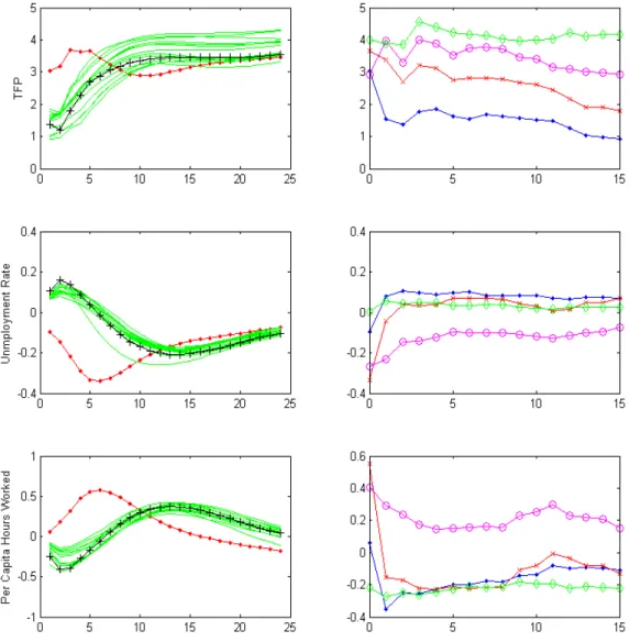
Figure 1 shows the impulse response functions. The left column plots the impulse response functions for the three varables, total factor productivity, unemployment and per capita hours, for all the sixteen specificationsz∗_t, w1_t, . . . , w_t15. The solid line with dots represents the impulse response functions estimated withz_t∗. The line with crosses represents the impulse response functions estimated withw2

t. The remaining lines are the estimated responses of the other models. The effects are expressed in percentage terms. The right column displays for the three variables the impact effect (dots),

the effect at 1 year (crosses), 2 years (circles) and in the long run (diamonds). The horizontal axis displays the number of principal components included in the VAR.

The VAR without principal components predicts that the technology shock increases per-capita hours worked and reduces unemployment. Such results are in line with the theoretical predictions of standard RBC models and the empirical findings of Chris-tiano, Eichenbaum and Vigfusson (2003) and Beaudry and Portier (2006). Total factor productivity reacts positively on impact and stays roughly constant afterward, with no delay in the diffusion process.

The picture changes dramatically when adding the principal components. The ef-fects on both unemployment and hours change sign. Now, unemployment increases and hours reduce so that technology becomes contractionary. Moreover, the impact effect of productivity reduces substantially while the long run effect is roughly unchanged so that the diffusion process is substantially slower in line with the S-shape view and the recent news shocks literature (Beaudry and Portier, 2006, and Schmitt-Grohe and Uribe, 2008).

Notice that, consistently with the results of the test, models including more than two principal components, all deliver the same impulse response functions. This can also be seen from the right panels of Figure 1. Impulse response functions change radically by adding the first principal component, and to a lesser extent by adding the second one, but are roughly constant from that point onward.

Figure 2 plots the impulse response functions of some variables of interest for the specificationw2_t. The solid line represents the point estimate while the dotted lines are the 68% confidence bands. Investment and GDP do not react significantly on impact and start to increase significantly only after a few quarters, reaching their maximal level after about two years. The shape of the response of consumption is similar to that of investment and GDP (although the impact effect is slightly negative). The GDP deflator reduces immediately while real wages immediately increase.

Overall the picture that emerges is hard to reconcile with the view that technology shocks are an important source of business cycle fluctuations.

4

Conclusions

This paper derives necessary and sufficient conditions under which a set of variables is informationally sufficient, i.e. contains enough information to estimate the struc-tural shocks with a VAR model. Based on such conditions, a procedure to test for informational sufficiency is proposed. Moreover, a test is provided to verify whether a single shock obtained with partial identification is a structural shock. Finally, the paper shows how to amend the model if informational sufficiency is rejected. The idea is to

estimate a FAVAR, where the number of factors is determined by applying recursively the sufficient information test.

Our testing procedures are applied to a three-variable VAR including TFP, unem-ployment and per-capita hours worked. It is found that the VAR is not informationally sufficient, and the technology shock, identified as the only one affecting TFP in the long run, is not a structural shock. When amending the model by adding missing informa-tion, informational sufficiency and structuralness cannot be rejected. Results in terms of impulse response functions change dramatically: the reaction of both unemployment and hours worked changes sign, so that a positive shock becomes contractionary, and the response of TFP becomes S-shaped, in accordance with the recent ”news” shock literature.

Appendix A: Proofs

Proof of Proposition 1. Sufficiency of (a) and (b) is obvious. As for necessity, let us assume that z∗_t is sufficient. Then from equation (6) and Assumption 3 we have P(z_t∗|Z_t∗₋₁) = P∞

k=1Fkut−k and t = W F0ut+W ξt, because ut−k ∈ Zt∗−1 and both

ut and ξt are orthogonal to Zt∗−1. Since ut = M t, M W ξt = 0, so that the variance-covariance matrix ofW ξt, say Σ, has rank l≤s−q. Hence Σ =Q0Q,Qbeing a l×s matrix of rankl. Let S be the l-dimensional subspace of Rs spanned by the rows of Q and R be any s−l×s matrix whose rows span the orthogonal complement of S. Clearly RW ξt = 0 and ˜zt=Rzt∗ =Rzt. Notice also that RW F0 has a left inverse N, so thatut =N Rt =M t, since otherwise ut cannot be a linear transformation of t, contrary to the informational sufficiency assumption.

Coming to (b), we want to show that Rt is the residual of the projection of ˜zt onto its own past, so that ut = N Rt ∈ Z˜t = span(˜zjt−k, j = 1, . . . , s−l, k ≥ 0). Let ¯zt = Qzt∗ and PK be the projection of ˜zt on the lags 1, . . . , K of ˜zt and ¯zt, i.e.

PK =P(˜zt|z˜jt−k,z¯ht−k, j = 1, . . . , s−l, h= 1, . . . , l, k = 1, . . . , K). First, observe that

z_t∗ is a linear combination of the entries of ˜zt and ¯zt, since the matrix (R0 Q0)0 is non-singular by construction. Hence PK → P(˜zt|Zt∗−1) = R

P∞

k=1Fkut−k in mean square as K → ∞. On the other hand, PK = CK(L)˜zt−1+DK(L)Qzt−1+DK(L)QW ξt−1. Therefore the latter term must go to zero in mean square asK → ∞. But QW ξt−1 is white noise by Assumption 2 and its variance-covariance matrixQΣQ0 is non-singular by construction, so that all entries ofDK(L) go to zero in sum of squares asK → ∞. It follows thatDK(L)Qzt−1 →0 andPK →P(˜zt|Z˜t−1) in mean squares asK → ∞. But then the latter projection is equal toRP∞

k=1Fkut−k, and the corresponding residual is

Rt. QED

Proof of Proposition 2. Assume that z_t∗ is sufficient, so that ut = M t. Then

ujt−k ∈ Zt∗−1 for k > 0. It follows that P(zt∗|Zt∗−1) = W(F1ut−1+F2ut−2+. . .) and t = W F0ut+W ξt. Hence t is orthogonal to both ut−k, k > 0, and, by serial uncorrelation of ξt (Assumption 2), ξt−k, k > 0. Therefore t ⊥ x∗t−k, k > 0 and x∗t

does not Granger causez∗_t . QED

Proof of Proposition 3. Let us assume that z_t∗ is sufficient, i.e. ut = M t. Then

t is orthogonal to ut−k, k > 0 and therefore to gt−k, k > 0. Hence P(zt∗|Zt∗−1) =

P(z_t∗|z_jt∗_−k, git−k, j = 1, . . . , s, i = 1, . . . , p, k > 0), so that gt does not Granger cause

z_t∗. Regarding the opposite implication, let us assume thatgt does not Granger cause

z_t∗. We have P(z_t∗|Z_t∗₋₁) = P(z_t∗|z_jt∗_−k, git−k, j = 1, . . . , s, i = 1, . . . , p, k > 0). But the latter projection is equal to P(z_t∗|ujt−k, j = 1, . . . , q, k > 0) = W

P∞

k=1Fkut−k =

ζt, since ζt belongs to span(zjt∗−k, git−k, j = 1, . . . , s, i = 1, . . . , p, k > 0) and zt∗ −

P(z_t∗|Z_t∗₋₁) =P∞

k=1Akt−k. Projecting both sums on span(it−k, uit−k, i= 1, . . . , s, j= 1, . . . , r) we getW Fkut−k=Akt−k for allk, so thatW Fkut=Aktfor allkandV ut= (WP∞

k=1ckFk)ut= (P∞k=1ckAk)t for any sequenceck,k = 1, . . . ,∞. Assumption 4 ensures thatV has a left inverse V∗, so that ut=V∗(P∞_k=1ckAk)t. QED

Appendix B: Data

Transformations: 1=levels, 2= first differences of the original series, 4 = logs of the original series, 5= first differences of the logs of the original series .

no.series Transf. Mnemonic Long Label

1 5 GDPC1 Real Gross Domestic Product, 1 Decimal

2 5 GNPC96 Real Gross National Product

3 5 NICUR/GDPDEF National Income/GDPDEF

4 5 DPIC96 Real Disposable Personal Income

5 5 OUTNFB Nonfarm Business Sector: Output

6 5 FINSLC1 Real Final Sales of Domestic Product, 1 Decimal

7 5 FPIC1 Real Private Fixed Investment, 1 Decimal

8 5 PRFIC1 Real Private Residential Fixed Investment, 1 Decimal 9 5 PNFIC1 Real Private Nonresidential Fixed Investment, 1 Decimal 10 5 GPDIC1 Real Gross Private Domestic Investment, 1 Decimal

11 5 PCECC96 Real Personal Consumption Expenditures

12 5 PCNDGC96 Real Personal Consumption Expenditures: Nondurable Goods 13 5 PCDGCC96 Real Personal Consumption Expenditures: Durable Goods 14 5 PCESVC96 Real Personal Consumption Expenditures: Services 15 5 GPSAVE/GDPDEF Gross Private Saving/GDP Deflator

16 5 FGCEC1 Real Federal Consumption Expenditures & Gross Investment, 1 Decimal 17 5 FGEXPND/GDPDEF Federal Government: Current Expenditures/ GDP deflator

18 5 FGRECPT/GDPDEF Federal Government Current Receipts/ GDP deflator

19 2 FGDEF Federal Real Expend-Real Receipts

20 1 CBIC1 Real Change in Private Inventories, 1 Decimal 21 5 EXPGSC1 Real Exports of Goods & Services, 1 Decimal 22 5 IMPGSC1 Real Imports of Goods & Services, 1 Decimal 23 5 CP/GDPDEF Corporate Profits After Tax/GDP deflator

24 5 NFCPATAX/GDPDEF Nonfinancial Corporate Business: Profits After Tax/GDP deflator 25 5 CNCF/GDPDEF Corporate Net Cash Flow/GDP deflator

26 5 DIVIDEND/GDPDEF Net Corporate Dividends/GDP deflator 27 5 HOANBS Nonfarm Business Sector: Hours of All Persons

28 5 OPHNFB Nonfarm Business Sector: Output Per Hour of All Persons 29 5 UNLPNBS Nonfarm Business Sector: Unit Nonlabor Payments

30 5 ULCNFB Nonfarm Business Sector: Unit Labor Cost

31 5 WASCUR/CPI Compensation of Employees: Wages & Salary Accruals/CPI 32 1 COMPNFB Nonfarm Business Sector: Compensation Per Hour

33 5 COMPRNFB Nonfarm Business Sector: Real Compensation Per Hour 34 1 GDPCTPI Gross Domestic Product: Chain-type Price Index 35 1 GNPCTPI Gross National Product: Chain-type Price Index 36 1 GDPDEF Gross Domestic Product: Implicit Price Deflator 37 1 GNPDEF Gross National Product: Implicit Price Deflator

no.series Transf. Mnemonic Long Label

38 5 INDPRO Industrial Production Index

39 5 IPBUSEQ Industrial Production: Business Equipment 40 5 IPCONGD Industrial Production: Consumer Goods 41 5 IPDCONGD Industrial Production: Durable Consumer Goods 42 5 IPFINAL Industrial Production: Final Products (Market Group) 43 5 IPMAT Industrial Production: Materials

44 5 IPNCONGD Industrial Production: Nondurable Consumer Goods 45 1 AWHMAN Average Weekly Hours: Manufacturing

46 1 AWOTMAN Average Weekly Hours: Overtime: Manufacturing 47 2 CIVPART Civilian Participation Rate

48 5 CLF16OV Civilian Labor Force

49 5 CE16OV Civilian Employment

50 5 USPRIV All Employees: Total Private Industries 51 5 USGOOD All Employees: Goods-Producing Industries 52 5 SRVPRD All Employees: Service-Providing Industries

53 5 UNEMPLOY Unemployed

54 1 UEMPMEAN Average (Mean) Duration of Unemployment

55 1 UNRATE Civilian Unemployment Rate

56 5 HOUST Housing Starts: Total: New Privately Owned Housing Units Started 57 1 FEDFUNDS Effective Federal Funds Rate

58 1 TB3MS 3-Month Treasury Bill: Secondary Market Rate 59 1 GS1 1-Year Treasury Constant Maturity Rate 60 1 GS10 10-Year Treasury Constant Maturity Rate 61 1 AAA Moody’s Seasoned Aaa Corporate Bond Yield 62 1 BAA Moody’s Seasoned Baa Corporate Bond Yield

63 1 MPRIME Bank Prime Loan Rate

64 5 BOGNONBR Non-Borrowed Reserves of Depository Institutions

65 5 TRARR Board of Governors Total Reserves, Adjusted for Changes in Reserve 66 5 BOGAMBSL Board of Governors Monetary Base, Adjusted for Changes in Reserve

67 5 M1SL M1 Money Stock

68 5 M2MSL M2 Minus

69 5 M2SL M2 Money Stock

70 5 BUSLOANS Commercial and Industrial Loans at All Commercial Banks 71 5 CONSUMER Consumer (Individual) Loans at All Commercial Banks 72 5 LOANINV Total Loans and Investments at All Commercial Banks 73 5 REALLN Real Estate Loans at All Commercial Banks

74 5 TOTALSL Total Consumer Credit Outstanding

75 5 CPIAUCSL Consumer Price Index For All Urban Consumers: All Items

76 5 CPIULFSL Consumer Price Index for All Urban Consumers: All Items Less Food 77 5 CPILEGSL Consumer Price Index for All Urban Consumers: All Items Less Energy

no.series Transf. Mnemonic Long Label

78 5 CPILFESL Consumer Price Index for All Urban Consumers: All Items Less Food & Energy 79 5 CPIENGSL Consumer Price Index for All Urban Consumers: Energy

80 5 CPIUFDSL Consumer Price Index for All Urban Consumers: Food 81 5 PPICPE Producer Price Index Finished Goods: Capital Equipment 82 5 PPICRM Producer Price Index: Crude Materials for Further Processing 83 5 PPIFCG Producer Price Index: Finished Consumer Goods

84 5 PPIFGS Producer Price Index: Finished Goods

85 5 OILPRICE Spot Oil Price: West Texas Intermediate

86 5 USSHRPRCF US Dow Jones Industrials Share Price Index (EP) NADJ 87 5 US500STK US Standard & Poor’s Index if 500 Common Stocks

88 5 USI62...F US Share Price Index NADJ

89 5 USNOIDN.D US Manufacturers New Orders for Non Defense Capital Goods (BCI 27) 90 5 USCNORCGD US New Orders of Consumer Goods & Materials (BCI 8) CONA 91 1 USNAPMNO US ISM Manufacturers Survey: New Orders Index SADJ 92 5 USVACTOTO US Index of Help Wanted Advertising VOLA

93 5 USCYLEAD US The Conference Board Leading Economic Indicators Index SADJ 94 5 USECRIWLH US Economic Cycle Research Institute Weekly Leading Index

95 1 GS10-FEDFUNDS

96 1 GS1-FEDFUNDS

97 1 BAA-FEDFUNDS

98 5 GEXPND/GDPDEF Government Current Expenditures/ GDP deflator 99 5 GRECPT/GDPDEF Government Current Receipts/ GDP deflator

100 2 GDEF Governnent Real Expend-Real Receipts

101 5 GCEC1 Real Government Consumption Expenditures & Gross Investment, 1 Decimal

102 1 Fernald’s TFP growth CU adjusted

103 1 Fernald’s TFP growth

104 5 DOW JOONES/GDP DEFL

105 5 S&P/GDP DEFL

106 1 Fernald’s TFP growth - Investment

107 1 Fernald’s TFP growth - Consumption

108 1 Fernald’s TFP growth CU - Investment

109 1 Fernald’s TFP growth CU - Consumption

110 1 Personal Finance Current

111 1 Personal Finance Expected

112 1 Business Condition 12 Months

113 1 Business Condition 5 Years

114 1 Buying Conditions

115 1 Consumer’s sentiment: Current Index

116 1 Consumer’s sentiment: Expected Index

References

[1] Bai, J., and S. Ng (2002). Determining the number of factors in approximate factor models, Econometrica 70, 191-221.

[2] Beaudry, P. and F. Portier (2006). Stock Prices, News, and Economic Fluctuations American Economic Review, 96(4): 1293-1307.

[3] Bernanke, B. S., J. Boivin and P. Eliasz (2005). Measuring Monetary Policy: A Factor Augmented Autoregressive (FAVAR) Approach, The Quarterly Journal of Economics 120, 387-422.

[4] Blanchard, O. J., and D. Quah (1989). The Dynamic Effects of Aggregate Demand and Supply Disturbances. American Economic Review, 79(4): 655-73

[5] Chari, V.V., Kehoe, P.J. and E.R. McGrattan (2008). Are structural VARs with long-run restrictions useful in developing business cycle theory? Journal of Mon-etary Economics 55: 1337-1352.

[6] Christiano, L., M. Eichenbaum and R. Vigfusson (2003), ”What Happens After a Technology Shock?”, NBER Working Papers 9819.

[7] Fernandez-Villaverde J., J.F. Rubio-Ramirez, T.J. Sargent and M.W. Watson (2007). ABCs (and Ds) of Understanding VARs. American Economic Review, American Economic Association, 97(3):1021-1026.

[8] Forni, M. and L. Gambetti (2010). Fiscal Foresight and the Effects of Government Spending, CEPR DP series no. 7840.

[9] Forni, Gambetti, L. and L. Sala (2010). News shocks do not drive the business cycle. Mimeo

[10] Forni, M., D. Giannone, M. Lippi and L. Reichlin (2009). Opening the Black Box: Structural Factor Models with Large Cross-Sections, Econometric Theory 25, 1319-1347.

[11] Forni M. and L., Reichlin (1996). Dynamic Common Factors in Large Cross-Sections, Empirical Economics 21, 27-42.

[12] Gal´ı, J. (1999), ”Technology, Employment and the Business Cycle: Do Technol-ogy Shocks Explain Aggregate Fluctuations?”,American Economic Review, 89(1): 249-271.

[13] Gambetti, L. (2010). Fiscal Policy, Foresight and the Trade Balance in the U.S. UFAE and IAE Working Papers 852.10.

[14] Gelper, S. and C. Croux (2007), Multivariate out-of-sample tests for Granger causality, Computational Statistics & Data Analysis 51, 3319-3329.

[15] Giannone, D., and L. Reichlin (2006). Does Information Help Recovering Struc-tural Shocks from Past Observations? Journal of the European Economic Associ-ation, 4(2-3), 455465.

[16] Hansen, L.P., and T.J. Sargent (1991). Two problems in interpreting vector autore-gressions. In Rational Expectations Econometrics, L.P. Hansen and T.J. Sargent, eds. Boulder: Westview, pp.77-119.

[17] Harvey, D. I., Leybourne, S. J. and P. Newbold, (1998) Tests for Forecast Encom-passing, Journal of Business & Economic Statistics 16, 254-259.

[18] Leeper, E.M., Walker, T.B. and S.S. Yang (2008). Fiscal Foresight: Analytics and Econometrics, NBER Working Paper No. 14028.

[19] Leeper, E.M., Walker, T.B. (2009). Information Flows and News Driven Business Cycles, mimeo Indiana University

[20] Lippi, M. and L. Reichlin (1993). The Dynamic Effects of Aggregate Demand and Supply Disturbances: Comment, American Economic Review 83, 644-652.

[21] Lippi, M. and L. Reichlin (1994). VAR analysis, non fundamental representation, Blaschke matrices, Journal of Econometrics 63, 307-325.

[22] Onatski, A. (2010). Determining the Number of Factors from Empirical Distribu-tion of Eigenvalues, The Review of Economics and Statistics 92, 1004-1016.

[23] Rozanov, Yu. (1967). Stationary Random processes. San Francisco: Holden Day

[24] Schmitt-Grohe, S and M., Uribe (2008). What’s News in Business Cycles, NBER WP 14215

[25] Sims, C. A. (1980). Macroeconomics and Reality. Econometrica, 48(1), 148.

[26] Stock, J.H. and M.W. Watson (2002a). Macroeconomic Forecasting Using Diffu-sion Indexes, Journal of Business and Economic Statistics 20, 147-162.

[27] Stock, J.H. and M.W. Watson (2002b). Forecasting Using Principal Components from a Large Number of Predictors, Journal of the American Statistical Associa-tion 97, 1167-1179.

[28] Yang, S.S. (2008). Quantifying tax effects under policy foresight. Journal of Mon-etary Economics, 52(8):1557-1568.

Tables

A B j z_t∗ w_t1 w_t2 z_t∗ w1_t w2_t 1 0.000 − − 0.005 − − 2 − 0.480 − − 0.055 − 3 0.405 0.475 − 0.113 0.977 4 − 0.620 0.375 − 0.091 0.452 5 − 0.125 0.250 − 0.115 0.581 6 − 0.105 0.500 − 0.142 0.641 7 − 0.125 0.545 − 0.126 0.186 8 − 0.285 0.785 − 0.027 0.197 9 − 0.125 0.705 − − 0.216 10 − 0.085 0.450 − − 0.207 11 − 0.050 0.660 − − 0.148 12 − − 0.355 − − 0.186 13 − − 0.395 − − 0.239 14 − − 0.560 − − 0.279 15 − − 0.720 − − 0.337

Table 1: p-values A: Test for informational sufficiency B: Test for structuralness of the technology shock.

Figures

RECent Working Papers Series

The 10 most RECent releases are:

No. 62 SUFFCIENT INFORMATION IN STRUCTURAL VARS (2011) M. Forni and L. Gambetti

No. 61 EXPORTS AND ITALY’S ECONOMIC DEVELOPMENT: A LONG-RUN PERSPECTIVE (1863-2004) (2011)

A. Rinaldi and B. Pistoresi

No. 60 THE WAGE AND NON-WAGE COSTS OF DISPLACEMENT: EVIDENCE FROM RUSSIA (2011)

H. Lehmann, A. Muravyev, T. Razzolini and A. Zaiceva

No. 59 INDIVIDUAL SUPPORT FOR ECONOMIC AND POLITICAL CHANGES: EVIDENCE FROM TRANSITION COUNTRIES, 1991-2004 (2011)

R. Rovelli and A. Zaiceva

No. 58 TRANSNATIONAL SOCIAL CAPITAL AND FDI. EVIDENCE FROM ITALIAN ASSOCIATIONS WORLDWIDE (2011)

M. Murat, B. Pistoresi and A. Rinaldi

No. 57 DYNAMIC ADVERSE SELECTION AND THE SIZE OF THE INFORMED SIDE OF THE MARKET (2011)

E. Bilancini and L. Boncinelli

No. 56 CARDINALITY VERSUS Q-NORM CONSTRAINTS FOR INDEX TRACKING (2011) B. Fastrich, S. Paterlini and P. Winker

No. 55 THE ATTRACTIVENESS OF COUNTRIES FOR FDI. A FUZZY APPROACH (2010)

M. Murat and T. Pirotti

No. 54 IMMIGRANTS, SCHOOLING AND BACKGROUND.CROSS-COUNTRY EVIDENCE FROM

PISA 2006 (2010)

M. Murat, D. Ferrari, P. Frederic and G. Pirani

No. 53 AGRICULTURAL INSTITUTIONS, INDUSTRIALIZATION AND GROWTH: THE CASE OF

NEW ZEALAND AND URUGUAY IN 1870-1940 (2010) J. Àlvarez, E. Bilancini, S. D’Alessandro and G. Porcile

The full list of available working papers, together with their electronic versions, can be found on the RECent website: http://www.recent.unimore.it/workingpapers.asp