Bloom maps for big data. David Talbot

Bloom maps for big data

David Talbot

Doctor of Philosophy

Institute for Communicating and Collaborative Systems

School of Informatics

University of Edinburgh

2009

Abstract

The ability to retrieve a value given a key is fundamental in computer science. Unfortunately as thea prioriset from which keys are drawn grows in size, anyexact data structure must use more space per key. This motivates our interest in approximate data structures. We consider the problem of succinctly encoding a map to support queries with bounded error when the distribution over values is known. We give a lower bound on the space required per key in terms of the entropy of the distribution over values and the error rate and present a generalization of the Bloom filter, the Bloom map, that achieves the lower bound up to a small constant factor.

We then develop static and on-line approximation schemes for frequency data that use constant space per key to store frequencies with bounded relative error when these follow a power law. Our on-line construction has constant expected update complexity per observation and requires only a single pass over a data set. Finally we present a simple framework for usinga prioriknowledge to reduce the error rate of an approxi-mate data structure withone-sidederror.

We evaluate the data structures proposed here empirically and use them to con-structrandomized language modelsthat significantly reduce the space requirements of a state-of-the-art statistical machine translation system.

This thesis would not have seen the light of day without a love of language and numbers that I picked up at an early age from my parents. Lacking most of the relevant skills for my chosen field, it would never have been completed without my brother’s patient help with the most basic of mathematical concepts.

My adviser, Miles Osborne, provided me with invaluable critical input throughout my time at Edinburgh, while at least giving me the impression that he trusted me to know what I was doing.

Finally, for helping me maintain a semblance of sanity, at least for public display, my biggest thanks goes to my best friend Daisuke.

Declaration

I declare that this thesis was composed by myself, that the work contained herein is my own except where explicitly stated otherwise in the text, and that this work has not been submitted for any other degree or professional qualification except as specified.

(David Talbot)

Table of Contents

2.2 Exact map data structures . . . 10

2.2.1 Lower bounds . . . 11

2.3 Approximate data structures . . . 13

2.3.1 Types of error . . . 13

2.3.2 Lower bounds . . . 14

3 Randomized data structures 19 3.1 Randomization . . . 19

3.1.1 Monte Carlo algorithms . . . 21

3.2 Hash functions . . . 22

3.2.1 Universal hash functions . . . 23

3.3 Loss functions . . . 25

3.3.1 Expected loss . . . 26

3.4 Tail bounds . . . 27

3.5 (ε,δ)-approximation schemes . . . 29

4 Previous work 31 4.1 Set membership testers . . . 31

4.2 Bloom filter . . . 32

4.2.1 Bloom filter error analysis . . . 34

4.3 A hash-based set membership tester . . . 37

4.5 Approximate maps . . . 40

4.5.1 Bloomier filter . . . 40

4.5.2 Other approximate maps . . . 41

4.6 Frequency look-up tables . . . 41

4.6.1 Spectral Bloom filter . . . 42

4.6.2 Bloom histogram . . . 42

4.6.3 Space-code Bloom filter . . . 43

5 Bloom maps 45 5.1 Space-optimal approximate maps . . . 45

5.2 The Simple Bloom map . . . 46

5.3 Efficient Bloom maps . . . 49

5.4 Reducing the constant factor . . . 59

5.5 Loss functions in a Bloom map . . . 60

6 Log-frequency Bloom filter 63 6.1 Frequency approximation schemes . . . 63

6.2 Log-frequency Bloom filter . . . 65

6.2.1 Main construction . . . 67 6.2.2 Error analysis . . . 68 6.2.3 An(ε,δ)-approximation scheme . . . 71 6.2.4 Optimizations . . . 72 7 Log-frequency sketch 73 7.1 Frequency estimation . . . 73

7.1.1 Approximate frequency estimation . . . 74

7.2 Approximate counting . . . 77

7.3 Approximate, approximate counting . . . 82

7.3.1 Estimation bias inapproximate, approximate counting . . . . 82

7.3.2 Bias correctedapproximate, approximate counting . . . 85

7.3.3 Bounded update complexity . . . 87

7.3.4 Optimizations . . . 89

7.3.5 Determining space usage . . . 90

8 Structured approximate maps 93

8.1 Structured key sets . . . 93

8.2 Structured key/value sets . . . 96

9 Empirical evaluation 99 9.1 Experimental set-up . . . 99

9.2 Bloom maps . . . 103

9.2.1 Bounding the 0-1 loss . . . 103

9.2.2 Using the distribution over values . . . 105

9.2.3 Usinga prioristructure . . . 107

9.3 Log-frequency Bloom filter . . . 110

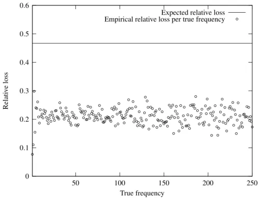
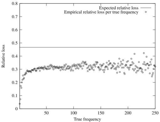
9.3.1 Bounding the relative loss . . . 110

9.3.2 Implementing a(ε,δ)-approximation scheme . . . 115

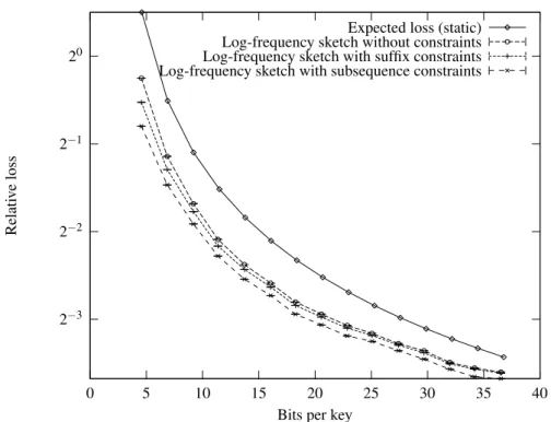
9.4 Log-frequency sketch . . . 120

9.4.1 Computational complexity . . . 124

9.5 Discussion . . . 124

10 Language models 127 10.1 Language models . . . 127

10.1.1 N-gram language models . . . 128

10.1.2 Parameter estimation . . . 129

10.1.3 Scalability . . . 132

11 Randomized language models 137 11.1 Approximaten-gram models . . . 137

11.2 Count-based models . . . 139

11.2.1 Stupid Back-off models . . . 140

11.2.2 Witten-Bell count-based models . . . 140

11.3 Back-off models . . . 143

11.4 Caching . . . 144

12 Language model experiments 147 12.1 Intrinsic evaluation . . . 147

12.1.1 Experimental set-up . . . 148

12.1.2 Count-based randomized language models . . . 151

12.1.3 Back-off randomized language models . . . 158

12.2.1 Experimental set-up . . . 163

12.2.2 Back-off randomized language models . . . 165

12.2.3 Count-based randomized language models . . . 166

12.3 Discussion . . . 167

13 Conclusions 173

A Notation 175

B General lower bound 177

C Power laws and logarithmic quantization 181

Bibliography 185

Chapter 1

Introduction

The ability to retrieve avaluegiven akeyis fundamental in computer science and real life. Retrieving birthdays given people’s names or names given faces; the key/value map is one of the most pervasive algorithms that computers and humans implement. Unfortunately key/value maps can become unwieldy in many practical situations. This thesis addresses this challenge by proposing a variety of approximate solutions and applying them to some practical problems in data processing.

Large key/value maps are commonplace in machine learning and data mining. This thesis grew out practical problems constructing one such map, ann-gram (i.e. Markov) language model for use in statistical machine translation. A language model maps word sequences to probability estimates. As with many key/value maps constructed from empirical data, language models are sparse(most possible word sequences do not appear) and the distribution of values within the map is skewed (most observed word sequences are rare but some are very frequent). Language models also exhibit structure sincea prioriconstraints may hold between related word sequences.

Previous work in the statistics community has focused on efficient model param-eterizations rather than directly addressing the space complexity of representing such models. Solutions proposed in the data structures literature, on the other hand, have failed to consider how either the distribution over values stored in a map or a priori information regarding the structure of the map can be used to improve the space/error trade-off of an approximate data structure. We attempt to fill some of these gaps by proposing data structures for representing key/value maps approximately that take into account both the distribution of the data anda prioristructure. These data structures may be suitable for a range of applications particularly in statistical data processing.

1.1

The Problem

We consider the problem of succinctly encoding a map such that values can be retrieved given keys. Lossless encoding of a large key/value map is problematic in many prac-tical settings since the space required to encode each key/value pair exactly increases as thea priorispace from which the keys are drawn grows in size. We will make this more precise in the following chapter. Consider first the simple but important problem of remembering your friends’ birthdays.

Imagine you were a rather unsociable person with very few acquaintances but wished to remain on good terms with a small group of good friends (a subset of your acquaintances). To avoid forgetting any of your friends’ birthdays, you record these next to their names in a notebook. Since none of your acquaintances has the same first initial, you decide to save paper by recording only the first letter of each friend’s name. Your friends, however, decide you should get out more often and introduce you to their friends. As your social circle broadens, this slowly undermines your space efficient notation scheme as you are forced to use more and more letters to identify friends drawn from this growing set of acquaintances in your notebook.

One day, you finally take the plunge and sign up to a social networking web site where you get to hang out virtually with people you’ve never even met. You have ‘friends’ now with the same initials, first names and even surnames. Your notebook is out of paper and you start to feel that something has to give.

This example gives some flavour of the problem we address in this thesis. We draw attention to the following characteristics in particular:

(Unbounded space) Whatever shorthand notation you devise, it seems unlikely that the space you use to denote each friend in the notebook can remain constant as your social circle grows.

(Space depends on thea prioriuniverse) Given no information as to which of your acquaintances is listed in your notebook, the amount of space you must use to denote each friend will dependnot on the number of people you choose to list there, but on the number of people among whom you need to distinguish.

In statistical data processing, large key/value maps arise perhaps more naturally. We often wish to estimate the frequency or probability of observations from some discrete set; in language modelling we are interested in word sequences. Many real data sets exhibit a power law distribution whereby a small number of events occur frequently while a large number occur rarely. Any model that attempts to describe this

1.1. The Problem 3 long tailof rare events will grow in size as more data and therefore more distinct events are observed. Ann-gram model is one such example.

Ann-gram language model is a key/value map from word sequences to probabil-ities. The larger the text used to build the model, the more distinctn-gram sequences we will observe and hence the more keys there will be in our map.

The space required to represent each key in ann-gram model exactly will depend on the number of distinct words observed in our training data, i.e. the vocabulary of the model. As the vocabulary grows, we must use more space pern-gram if we are to distinguish between them without error.

Approximate map data structures, as considered in this thesis, allow us to address the per-key space complexity of representing a map. If we are willing to accept that on occasion our data structure may return the wrong value for a key, then we can store key/value pairs in space that isindependent of the size of the a priori universe from which the keys are drawn. This fundamentally alters the space complexity of building such models as the amounts of available training data increase.

Given our interest in statistical data processing, we focus on aspects of the approx-imate map problem that are particularly relevant to such applications but have been overlooked in the more general data structures literature:

(i) Using the distribution over values in the map to optimize space usage;

(ii) Usinga prioristructure in the key/value data to reduce errors;

(iii) Incorporating explicit loss functions into an approximate map.

In many key/value maps encountered in statistical data processing values are ob-served to follow a skewed distribution. By using knowledge of the distribution, we may hope to reduce the space usage of an approximate map in much the same way as lossless encoding schemes compress low entropy data more readily.

Many data sets exhibit significant structure that can be encoded as a priori con-straints on the values that can correctly be retrieved from the map. We consider how to use such constraints to improve the space/error trade-off of an approximate map.

Finally, the impact that errors have on an application may vary significantly be-tween applications. Existing approximate map data structures allow only the 0-1 loss or probability of error to be bounded. We consider how a wider variety of loss func-tions could be incorporated within an approximate map data structure.

1.2

Contributions

We give a novel lower bound on the space complexity of representing a key/value map approximately with bounded error when the distribution over values is known. These generalize a lower bound on the set membership problem [Carter et al. (1978)] and demonstrate that we can remove the space dependency on the size of thea priori universe from which keys are drawn to store a map in constant space per key if errors are allowed.

Our main practical contribution is a series of data structures for various versions of the approximate map problem. The data structures that we propose all naturally lever-age the distribution over values stored in a map to achieve significant space savings over previous general solutions to the approximate map problem.

We introduce theBloom map, a simple generalization of theBloom filter [Bloom (1970)], that solves the approximate map problem within a small constant factor of the lower bound. A Bloom map representing a map with bounded 0-1 error uses constant space per key where the constant depends only on the entropy of the distribution over values in the map and the probability of retrieving the wrong value for a key. We give Bloom map constructions that allow a range of space/time trade-offs for a given error rate and describe how a Bloom map can be constructed with boundedabsoluteloss.

We present two approximate data structures for representing frequency data. The log-frequency Bloom filter can encode a static set of key/frequency pairs in constant space per key with bounded relative loss when the frequencies follow a power law. Thelog-frequency sketchallows frequencies to be estimated on-line from a single pass over a data set with bounded relative loss. It uses constant space per key and has constant expected update complexity per observation. This data structure adapts the approximate countingalgorithm [Morris (1978)] to work with an approximate map.

We then present a framework for incorporatinga prioriconstraints into an approx-imate map algorithm. This framework makes use of the fact that our approxapprox-imate map data structures haveone-sidederrors to allow the results of multiple queries of a data structure to constrain one another when we havea prioriknowledge regarding the re-lations that must hold between values for related keys. This allows us to reduce the error rate of an approximate data structure in practice when sucha prioriinformation is available.

To corroborate claims made for the data structures proposed here and to demon-strate the impact of incorporatinga prioriconstraints based on real data, we present a

1.3. Outline 5 range of empirical evaluations of these data structure usingn-gram frequency data.

Finally as a more involved application of the proposed data structures, we use them to implement n-gram language models. This gives us a benchmark application on which to validate the performance of our data structures and allows us to explore the choices available when constructing a statistical model on top of an approximate map. We present experiments evaluating how the space/error trade-off of arandomized language modelis affected by the choice of underlying parameterization scheme. We also demonstrate that the approximate map data structures that we have proposed can be used to significantly reduce the space requirements of a state-of-the-art statistical machine translation system.

1.3

Outline

The next chapter formulates the approximate key/value map problem and presents our lower bounds. Chapters 3 and 4 then introduce some concepts from the field of ran-domized algorithms and review related work on approximate data structures.

In Chapters 5, 6 and 7 we present novel data structures for the key/value map problem, and static and on-line approximation schemes for frequency data. In Chapter 8 we describe howa prioriconstraints may be incorporated into these data structures.

We evaluate our data structures empirically in Chapter 9. Then, after a brief review of statistical language models in Chapter 10, describe how they can be used to imple-ment succinct language models in Chapter 11. We evaluate these randomized language models in Chapter 12 and conclude with some directions for future work.

Chapter 2

Approximate maps

We start by defining the key/value map problem and motivating our interest in approx-imate solutions by giving lower bounds on the space complexity of any exact solution. We consider the different types of error an approximate map may make and present lower bounds on the space complexity of any data structure that implements a map with bounds on each type of error. These lower bounds were presented previously in Talbot and Talbot (2008).

2.1

Problem statement

We will use the following definition of a key/value map in this thesis.

Definition 2.1. Akey/value mapis a functionM:U →V∪ {⊥}whereU is theinput space, V is the value set and ⊥ is the null value. |U|=u, |V|=b and the support S={x∈U|M(x)∈V}has sizen. Akeyis an elementx∈U.

We assume that the functionM is specified by the designer of the map. One way to specifyMis to provide a set of key/value pairs for the supportS

M={(x1,v(x1)),(x2,v(x2)), . . . ,(xn,v(xn))}

where v(x)∈V is the value associated with a key x∈S and x∈U\S is implicitly mapped to⊥. This is a common way to define a map ifU is much larger thanS.

For example, given a set of friends’ names S and days of the year V, we could define a map M that associates each friend x∈S with their birthday v∈V to help us remember them. The input space to the mapU could be defined as the set of all possible names of which our friends’ names S would constitute a subset S⊂U. We

would naturally map names of people we did not know x∈U\S to⊥ which in this case would signifyunknown.

The key/value map framework covers various other data structure problems. For example, by settingV ={true}and letting⊥signifyfalse, we obtain aset membership testerthat identifies whetherx∈Uis a member of a setS. Similarly by settingV =_Z+ we obtain afrequency look-up tablethat maps objectsx∈U to their countsc∈V with

⊥naturally indicating a zero count.

In the following we will often make use of the distribution~p={p₁,p₂, . . . ,p_b}

over valuesv∈V stored in a map (i.e. the fraction of keysx∈Sthat are assigned each valuev∈V). While this restricts our results to cases where this distribution is known (at least approximately) this knowledge allows us to derive sharper lower bounds on the problem and, as we will see in later chapters, allows us to optimize the space usage of the data structures that we propose. Previous work on the approximate map problem has not considered how this distribution determines both the lower and upper bounds on this problem.

To make the knowledge of the distribution explicit in our discussion, we will intro-duce the concept of a~p-map: a map with a fixed and known distribution over values.

Definition 2.2. A~p-map is a key/value mapM :U →V∪ {⊥} as defined above for which the distribution~p={p₁,p₂, . . . ,p_b}of values assigned to keys is known (clearly ∑b_i=1pi=1 and mini∈[b]pi>0). Thus ifSi={x∈S|M(x) =vi}then|Si|=pin.

We assume the following for the classes of map considered in this thesis.

(i) (Unbounded input space)|U|is not constant as a function of|S|;

(ii) (Sparse support)Sis much smaller thanU (technically limn→∞n_u →0);

(iii) (Fixed value set)V is constant.

Assumption (i) refers to a sequence of key/value maps arising for a given problem; it must hold for the space complexity of the problem to be of interest: if |U| remains fixed for all key/value maps from a given class then we can always identify keysx∈U using the same amount of space. The assumption is valid in many applications in data processing where|U|increases as the amount of data grows.

Commonly we use some knowledge regardingSto constrain the input spaceU. In the simple case whereU are strings, for instance, we may defineU via a restriction on the maximum string length in S: clearly if we know that no keys in the support S

2.1. Problem statement 9 are longer than 5 characters then we can exclude all longer keys prior to querying the map. However, as we observe more strings that we wish to include inSthen we may expect the maximum string length inSto increase and therefore the size ofU to grow exponentially.

OftenU is defined combinatorially from elements of an underlying alphabet, for instance, words combining asn-grams in text processing or IP addresses combining as flow patterns in network analysis. A prior procedure in this case, might be to check that each atomic unit in the input key is a valid member of the alphabet restricted to el-ements occurring inS. While this procedure may require significantly more space than the above restriction on the maximum string length, it may be insignificant compared to the space required to represent the map. As we observe more data,U may increase due to growth in the underlying alphabet (new words or IP nodes are observed) or from a desire to model higher-order combinations given larger amounts of data.

Assumption (ii) extends assumption (i): not only isU growing withS but its rate of growth is faster than that of the support; henceSis a vanishingly small fraction of the input space. Clearly this is true if |U| has an exponential dependency on some aspect of the support. For example, if Sconsists of empirically observed strings and we increase the size ofU by allowing it to include longer strings to ensure that the support S remains a subset ofU, we will not normally expect all possible strings of this length to occur. In many natural examples as |U| grows the fraction of U that we expect to observe decreases. This type of phenomena occurs naturally for data distributed according to a power law. In language modelling, for instance, the space of possiblen-gramsU increases exponentially in the ordernwith the base determined by the vocabulary size (i.e.U =|

V

V

distinctn-grams observed in practice grows much less rapidly.

Assumption (iii) is less important for the results presented in this thesis and is primarily needed to keep the analysis simple. Clearly for a given family of~p-maps, since~p(the distribution over values) is assumed fixed and known,V must be constant. There are many examples of maps for which the set of values is constant while the set of keys may be unbounded (e.g. names and birthdays). Our results show that ifV is increasing then we cannot represent a map in constant space even approximately with bounded error, hence approximation schemes are less interesting in such cases.

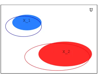
Figure 2.1: An exact map with two values.

2.2

Exact map data structures

An exact map data structure must implement the function M for x∈U as specified by the designer of the map. In other words, (to continue the earlier example) given a namex∈U, an exact encoding ofM would return the corresponding friend’s birthday ifx∈Sand⊥otherwise. An exact encoding ofM must not forget any of our friends’ birthdays or indeed forget any of our friends; it must also not spuriously claim to know the birthdays of people we have never met. A Venn diagram of an exact map with two values is depicted in Fig.( 2.1).

The definition of a map itself may already include ‘approximations’ which it is important to differentiate from such errors. For instance, we may have, in defining the map, decided that since our friends have a tendency to forget our birthday, we need only remember the week in which each of their birthdays fall to remain on amicable terms. This would reduce the size ofV from 365 (the number of days in the year) to 52 (the number of weeks). More generally we may wish to define either the input spaceU and/or the value setV by partitioning a larger set into a smaller number of equivalence classes. This could be for reasons ranging from statistical efficiency or noise reduction right through to simply wishing to save space.

Approximations that are inherent in the specification ofM will mostly be ignored and if necessary will be referred to as model-based approximations: we assume that these are explicitly controlled by the designer of M. Such approximations are com-monplace in statistical modelling. Whether or not the specification of a map introduces model-based approximations is entirely independent of whether it is implemented by

2.2. Exact map data structures 11 an exact map data structure. Of course, in practice we may wish to consider the inter-action of approximations both in the specification and the implementation ofM.

Before we look at approximate solutions to encoding a key/value map, we should first explain why we do not wish to limit ourselves to exact solutions to this prob-lem. Below we present information theoretic arguments that expose the limitations of lossless data structures in representing a map whenU is unbounded. The following dis-cussion extends ideas presented in Carter et al. (1978) for the set membership problem and introduces the framework in which we will prove lower bounds on approximate data structures later in this chapter.

2.2.1

Lower bounds

The fundamental problem with any exact encoding of a key/value map is its space complexity. No lossless data structure can hope to represent a key/value map in con-stant space per key as the size of the input spaceU grows. Intuitively it makes sense that in order to encode a key/value map exactly we must be able to distinguish between all possible keysx∈Uthat may be presented to the data structure (if not then we must make errors) and to assign distinct identifiers tox∈U must require space that depends on|U|(given noa prioriknowledge of the structure ofU).

To make this more formal we consider a counting argument that gives a lower bound on the space required to encode all~p-maps for a fixed input spaceU, a fixed size supportnand a fixed distribution~pover the assignment of values to keys. Having fixed a familyof~p-maps in this way (i.e. the set of all distinct~p-maps that can be defined over this input space with support of size n), a lower bound on the space complexity of any data structure that can encode all ~p-maps in this family without error is also a lower bound on the space needed by any algorithm that guarantees to encode any

~p-map from this family without error and without additionala prioriknowledge: we do not assume that we know a priori which~p-map in this family we wish to encode and hence we must ensure that our data structure has enough space to encode any map from this family distinctly.

To continue the previous example, this is a lower bound on the amount of space required by any data structure that guarantees to return the correct birthdays for all our friends givena priorionly the input spaceU, the number of friends we havenand the distribution over their birthdays~p. Clearly if, we had other a priori knowledge (for instance if we already knew which members ofU were our friends, or that they were

all born in August) then this lower bound would no longer apply.

The proof of the following theorem uses a counting argument from Carter et al. (1978) that we apply later to obtain lower bounds on the approximate map problem. We assume that we have access to a deterministic algorithm that takes as input anm-bit string s and a keyx∈U; the algorithm then returns a value v∈V ∪ {⊥}. Since the algorithm is deterministic, it must return the same valuevwhenever it is presented with the same stringsand keyx∈U.

A string s encodes a map M exactly if, given s and a key x∈U, the algorithm returns the correct value for x according to the mapM. To obtain a lower bound we determine how many distinct~p-maps a given stringsmay encode and relate this to the total number of~p-maps in the family.

Theorem 2.1. Any data structure that can encode all ~p-maps exactly given a fixed input space U of size u, support of size n, value set V and distribution over values~p must use at least

m=logu−logn+H(~p) +o(1) bits per key.

Proof. To encode all ~p-maps in the family without error, we must use one string to specify each~p-map. If one string were used to encode more than one distinct~p-map then it would necessarily assign the wrong value to at least one key in one these~p-maps (since they are distinct and the algorithm is deterministic). There are

u n n p1n,p2n, . . . ,pbn

~p-maps for fixed input space of sizeu, support of sizenand distribution over values

~p; the first term is the number of distinct ways that we can select the support from the input space (i.e. choose our friends) and the second term is the number of distinct ways that we can assign values to the elements of the support according to the distribution~p (i.e. possible assignments of birthdays to friends for this distribution).

There are 2m distinct binary strings of lengthmand therefore to assign one string to each~p-map we must have

2m≥ _u n _n p1n,p2n, . . . ,pbn .

Since u_nis at least (u_n)n and by Stirling’s formula the multinomial coefficient is ap-proximately 2nH(~p)+O(logn)(whereH(~p)is the entropy of the distribution over values), the result follows by taking logarithms and dividing by the size of the supportn.

2.3. Approximate data structures 13 The lesson of Theorem 2.1 is that exact solutions to the key/value map problem must use space that depends on the size ofU in general. WhenU is unbounded as a function of S, this implies that we cannot encode key/value pairs in constant space. More worryingly, perhaps, in data processing, is that although U may be growing much faster than the support S, the latter may in fact also be growing very quickly. Hence maps induced on increasing amounts of data may grow very rapidly due to the combined increase in the number of keys in the support and the space required to represent each such key/value pair.

2.3

Approximate data structures

We now turn to the main focus of this thesis: approximate map data structures. A data structure which is explicitly allowed to make errors has a fundamental advantage over any exact data structure: it need not distinguish between all inputs x∈U. This allows an approximate data structure to circumvent the space dependency on the size of the universeu, identified above as a fundamental limitation of an exact data structure when the support S is growing. In the remainder of this thesis we will use the term ‘approximate map data structure’ in the following slightly restricted sense.

Definition 2.3. Anapproximate map data structure Mˆ for a map M defined over an input spaceU is one which when queried with a random inputx∈U has a non-zero butquantifiedprobability of returning the wrong valuev∈V∪ {⊥},v6=M(x)(where M(x)is the value specified by the designer of the map).

This definition captures the two most important characteristics of an approximate data structure for our purposes: (i) it may return incorrect (and unexpected) values; (2) the probability that it makes such errors isexplicitly quantified. To be of practical use in a given application, we must be able to control the probability of error for an approx-imate map, ensuring it is not excessive for the given application. The error rate of all data structures considered in the remainder of this thesis permit a space/error trade-off whereby the error of the data structure can be made arbitrarily small by increasing its space usage.

2.3.1

Types of error

Below we will present lower bounds on the space requirements of any data structure that implements an approximate map with bounded error. These lower bounds will

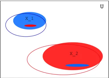
depend (to some extent) on the type(s) of error that the approximate map is allowed to make. We consider the three distinct types of error depicted in Venn diagrams in Figs. (2.2), (2.3) and (2.4). Recalling our previous notation: U is the input space, S is the support, S_i is the subset of S that mapped to v_i∈V by M and U\S is the complement of the support which is mapped to⊥byM. An approximate map ˆMmay make various types of error which we now define.

Definition 2.4. The errors of an approximate map ˆMcan be categorized as follows:

• (False positives) x∈U\Sis incorrectly assigned a valuev∈V;

• (False negatives) x∈Siis incorrectly assigned the value⊥;

• (Misassignments) x∈Siis incorrectly assigned a valuev∈V\ {vi}.

For an approximate map ˆMand fori∈[b]we also define the followingerror rates that we use to quantify the above types of error.

Definition 2.5. Thefalse positive rate, false negative rateandmisassignment rate of an approximate map ˆMare computed as follows

f+(Mˆ) = |{x∈U\S|Mˆ(x)6=⊥}| |U\S| , (2.1) f_i−(Mˆ) = |{x∈Si|Mˆ(x) =⊥}| |Si| , (2.2) f_i∗(Mˆ) = |{x∈Si|Mˆ(x)∈V\ {vi}}| |S_i| . (2.3)

Thus f+(Mˆ)is the proportion of keys inU\Sthat result in a false positive; f_i−(Mˆ) is the proportion of keys inS_ithat result in a false negative; and f_i∗(Mˆ)is the proportion of keys inS_ithat are misassigned their value.

These distinct types of error each affect the space complexity of an approximate map differently. Given the query distribution~q= (q1,q2, . . . ,qb,q⊥) where qi is the

probability that we query valuevi, the error rates defined above could be used to

com-pute the 0-1 loss of ˆM. Later we will consider other loss functions that may be more suited to maps defined over ordered sets of valuesV.

2.3.2

Lower bounds

We now present lower bounds on the approximate map problem that demonstrate how the space complexity of the approximate version differs from its exact version. These

2.3. Approximate data structures 15

Figure 2.2: An approximate map with false positives.

Figure 2.4: An approximate map with false positives, false negatives and misassign-ments.

lower bounds, presented previously in Talbot and Talbot (2008), highlight two impor-tant aspects of the approximate map problem as well as providing a useful benchmark for the approximate map data structures we present in later chapters.

(i) Key/value maps can be stored in constant space per key when errors are allowed;

(ii) Allowing false positives is sufficient to remove the dependency onu;

(iii) False negatives and misassignments have little effect on the space complexity.

Definition 2.6. Given constantsε+ >0 andε∗,ε− ≥0 we will a strings(ε+,ε∗,ε−) -encodes M if it satisfies: f+(s)≤ε+ and, for all i∈[b], f_i∗(s)≤ε∗ and f_i−(s)≤ε−. (We will assume throughout that max{ε+,ε∗,ε−}<1/8.)

If the only errors we allow are false positives then we have an(ε+,0,0)-encoding data structure. Theorem 2.2 gives a lower bound on the space requirements of such a data structure. The proof makes use of the counting argument presented above and gen-eralizes the argument applied to the approximate set membership problem by Carter et al. Carter et al. (1978).

Theorem 2.2. The average number of bits required per key in any data structure that (ε+,0,0)-encodes all~p-maps is at least

2.3. Approximate data structures 17 Proof. Suppose that the m-bit string s (ε+,0,0)-encodes some particular ~p-map M with key setX. Fori∈[b]let A_i(s)={x∈U |s(x) =vi}, a(_is)=|A(_is)|and defineq(_is)

bya(_is)=pin+ε+(u−n)q(_is). SinceXi={x∈X |v(x) =vi}has size pinandsalways

answers correctly onX_iwe haveq(_is)≥0.

The proportion ofx∈U\X for whichs(x)6=⊥is∑bi=1ε+q (s)

i . Since f

+_(s)≤ ε+, this implies that∑b_i=1q(_is)≤1.

IfN is any~p-map with key setY that is also (ε+,0,0)-encoded by sthen, sinces correctly answers all queries on keys in Y, we haveYi={y∈Y |v(y) =vi} ⊆A(_is),

for all i∈[b]. Hence, since |Yi|= pin, s can (ε+,0,0)-encode at most the following

number of distinct~p-maps

b

∏

∏

Choosing q₁,q₂, . . . ,q_b ≥0 to maximize this expression, subject to ∑b_i=1qi≤1, we

must have 2m b

∏

Using the fact that (a−b_b!)b ≤ a_b

≤ ab

b! and taking logarithms we require m+

b

∑

i=1

p_inlog(p_in+ε+(u−n)qi)≥nlog(u−n).

Dividing byn, recalling that∑b_i=1pi=1 and rearranging we obtain

m n ≥log 1/ε +₊ b

∑

∑

Our assumption that un(which is equivalent ton/u=o(1)) together with the fact that log(1+α) =O(α)forαsmall implies that the last two terms areo(1). Hence the average number of bits required per key satisfies

m n ≥log 1/ε +₊ b

∑

Gibbs’ inequality implies that the sum is minimized whenqi = pi for alli∈[b], the

result follows.

This calculation can be extended to the case when false negatives and misassign-ment errors are also allowed on keys in the supportS.

Theorem 2.3. The average number of bits required per key in any data structure that (ε+,ε∗,ε−)-encodes all~p-maps is at least

(1−ε−)log 1/ε++ (1−ε−−ε∗)H(~p)−H(ε−,ε∗,1−ε−−ε∗) +o(1).

Proof. The basic idea behind the proof of this result is the same as that of Theorem 2.2, however the details are somewhat more involved. It is presented in Appendix B.

This general lower bound on the approximate map problem reveals the different impact that the three distinct types of error (false positives, false negatives and misas-signments) have on the problem. While allowing false positives fundamentally alters the space complexity of representing a key/value map by removing the dependency on

|U|, false negatives and misassignments play a somewhat smaller role.

False negatives simply reduce the space complexity of the problem in a linear fash-ion as is perhaps obvious. By allowing false negatives we store a map ˆMthat has sup-port of sizenε−rather than the original mapMwith support of sizen. We can achieve this space complexity in practice simply by choosingnε− keysx∈Sto discard.

Misassignments allow us to reduce only the entropy term. Irrespective of the bound on the misassignment rate ε∗, we still require log 1/ε+ bits per key to deter-mine whether an element is contained in the map without exceeding the proscribed false positive rate. Again the result is intuitive: as the misassignment rate approaches 1 the entropy term tends to zero as we fail to associate any information with each of the keys stored in the map other than identifying them as members of the support.

Chapter 3

Randomized data structures

Randomization features heavily in the design of approximate data structures and algo-rithms; it often plays a crucial role in reducing the complexity of a problem or sim-plifying the analysis of an algorithm. In this chapter we review some of the roles of randomization in designing algorithms more generally and consider loss functions suitable for quantifyingapproximation schemesimplemented by the data structures we present in later chapters.

3.1

Randomization

Arandomized algorithmis one that requires access to a sequence of random bits in ad-dition to its main input. Randomization is used by all of the approximate data structures considered in this thesis although a randomized algorithm need not be approximate and an approximate data structure need not be implemented by a randomized algorithm.

Randomization might be expected to complicate the analysis of an algorithm; in practice, the opposite is usually true. A common motivation for introducing random-ization into an algorithm is to simplify its analysis and/or make it robust to uncertainty regarding the input distribution. Classical computer science favours worst-case analy-sis of algorithms; in many cases, if we knew the distribution over inputs, an average-case analysis might be more reasonable. Randomization can sometimes bring the two approaches closer together.

The running time and space usage of any algorithm (randomized or deterministic) is a random variable when the input to the algorithm is unknown. Introducing explicit randomization into an algorithm can allow us to control the distribution of this random variable more directly insulating the algorithm from uncertainty in the input.

A deterministic version of the divide-and-conquer sorting algorithmquick-sort, for instance, might always choose the midpoint in a set of data as its pivot to perform comparisons at each stage; it would therefore have a fixed running time given a fixed input. However, for some worst-case input the running time will be O(n2). We can compute the expected running time of deterministic quick-sort, if we have access to or make assumptions about the distribution over inputs to the algorithm. For instance, if we assume that all inputs are equally likely then the deterministic algorithm has an expected running time of Θ(nlogn); if the distribution is not uniform, however, our analysis may be way off the mark.

A randomized version of quick-sort can be obtained by selecting the pivot element uniformly at random at each stage. The running time of this algorithm even on a fixed input is now a random variable since the exact time required to sort the data will depend on which pivot elements are sampled during its execution. The expected running time of this algorithm, however, on any inputis now Θ(nlogn)since a random pivot point will on average provide a good (i.e. balanced) split of the data.

The introduction of random choices into the algorithm renders its running time in-dependent of either the input distribution or any specific input. We have moved the ran-domness from the input distribution (i.e. uncertainty regarding the order of the input) to the choice of pivot point. Hence the uniform analysis for the deterministic algorithm holdswith no distributional assumptionsfor the expected behaviour of the randomized algorithm on any input. The underlying principle here is that a random function of any input (random or non-random) is random and hence having applied a random function to the input, we need no longer be concerned with its initial distribution.

The random variable (e.g. running time, space usage, error rate etc.) resulting from such anexplicitlyrandomized algorithm can often be analysed very precisely. In addi-tion to computing the expected value of various aspects of such an algorithm, a range of techniques from probability theory allow us to bound the tail of the distribution thereby quantifying the probability that the variable deviates from its expected value [e.g. Motwani and Raghavan (1995), Chapters 3 and 4]. In many cases, for instance when the analysis results in sums of independent or Markov random variables, an ex-tremely powerful phenomena known as theconcentration of measuremay imply that the resulting variable has only an exponentially small probability of deviating from its mean (for all intents and purposes the variable is equal to its expected value). McDi-armid (1999) has shown this to be the case for the running time of quick-sort. Hence an explicitly randomized algorithms may admit a simpler and more precise analysis

3.1. Randomization 21 than a ‘conventional’ algorithm in which the only randomness is uncertainty regarding the input distribution.

3.1.1

Monte Carlo algorithms

Randomized algorithms are often categorized as Las Vegas or Monte Carlo. Ran-domized quick-sort is an example of the former: the output is always correct but the running time of the algorithm is a random variable. In a Monte Carlo algorithm, the output itself is a random variable and has non-zero probability of being incorrect. The randomized data structures proposed in this thesis are all Monte Carlo algorithms.

For decision problems (i.e. problems where the output isx∈ {yes,no}), it is com-mon to distinguish two types of Monte Carlo algorithm depending on the type of error that the algorithm is allowed to make. An algorithm is said to have one-sided error if it makes errors only in one direction; for example, it never makes errors on inputs for which the output should benobut may make errors on inputs for which the output should beyes. One-sided error can be an extremely useful property for an algorithm, particularly when combined with independent random choices.

One motivation for introducing randomness into an algorithm is to render suc-cessive calls to the algorithm independent of one another; this is particularly useful when any single call could result in an error but this error depends only on the random choices made on that particular call. If, in addition, the error made by the algorithm is one-sided, then by repeating the algorithm multiple times with different random bits we can make the probability of error arbitrarily small.

Perhaps the most famous application of this principle is in primality testing. A primality tester should answer yes given an input x that is prime and no otherwise. Given an input x there exists a very simple Monte Carlo primality tester with one-sided error that takesxand a random integeraless thanx. The algorithm usesato test certain properties ofxdetermining whetherxis eitherdefinitely notprime orpossibly prime. If the output of this algorithm isnothen we are guaranteed thatxis not prime; if the output of this algorithm isyesthen it is correct at least 1/2 the time (this error is one-sided). This probability of error is over the choice ofa: at least half of all integers less thanxwill not result in an error when used to check whetherxis prime.

To reduce the error of such an algorithm to an arbitrarily small value, we simply repeat the algorithm with distinct random choices of a. When repeated t times, the algorithm will either outputnoat some point at which we can immediately stop since

this is guaranteed to be the correct output, or it will outputyeson each call and will be expected to make an error over alltcalls with probability 1/2t(essentially never if, say, t>100). This follows from the fact that the algorithm’s behaviour depends only on the sequence of integers chosen to perform the test and these are sampled independently at random on each call. Until recently this was the only known polynomial time algorithm for primality testing.

3.2

Hash functions

The approximate data structures proposed in this thesis make heavy use of both aspects of randomization highlighted above: (i) a random function maps inputsuniformlyand therefore can insulate an algorithm from the input distribution and (ii) distinct random functions are independent of one another and hence so are any resulting errors. In practice we will userandom hash functionsto randomize our data structures. We now review the concept of a random hash function and describe a class of practical hash functions used by the data structures proposed in this thesis.

A hash functionh:U→[0,M−1], e.g. Morris (1968), maps keys from a universe U of sizeu to integers in the range [0,M−1]. We will assume thatu>M. A hash function is a deterministic function in that it maps an element x∈U to the samei∈

[0,M−1]on each call. Hash functions are commonly used to disperse elements from U uniformlyover the range[0,M−1]; by this we mean that each integeri∈[0,M−1] should be the output of (approximately) the same number of elements inU.

Collisions, whereby two distinct keysx,x0∈U are assigned to the same integeri∈

[0,M−1], will occur for all hash functions by the pigeon-hole principle whenu>M. In most randomized algorithms, we wish to analyse the probability of such collisions under our hash functions. To remove any dependency on the input distribution (the distribution over keys), we generally assume that we have access to truly random hash functions for which the probability that any key x∈U is mapped to any integer i∈

[0,M−1]is 1/M. This implies that all integers in[0,M−1]will be selected with equal probability for any input distribution; randomization plays precisely the same role here as it did for randomized quick-sort described above. In practice, therandomness of a hash function is derived from the fact that certain (pseudo-)random choices are made when it is initialized, i.e. the selection of certain parameters.

The data structures proposed in this thesis use hash functions to map keysx∈U (somewhat indirectly) to values v∈V ∪ {⊥}. A given instantiation of such a data

3.2. Hash functions 23 structure maps any key x∈U to the same value each time it is queried. However, since each instantiation of the data structure will select its own set of hash functions at random from a suitable family, collisions will occur for different sets of keys x∈

U on different instantiations. In analysing such a data structure’s performance, we consider the probability of particular collisions when constructing and querying the data structure where the uncertainty is over the choice of random hash functions for a given instantiation. By assuming that any hash function from the family will disperse keys approximately uniformly over the range [0,M−1], we can render the analysis independent of both the choice of the supportS⊂U for any given map and the exact choice ofx∈U with which the data structure is queried. We will return to this below when discussing the concept ofexpected lossfor such a data structure.

Assuming access to a random number generator, a simple random hash function can be constructed using a look-up table with u entries where each entry contains a random number in the range [0,M−1]. Evaluating the function for input x∈U is a simple look-up of the value stored in cellxof this table. To store this table, however, would require O(ulogM)bits which is prohibitive whenuis large, precisely the case of interest.

Fortunately functions that possess some of the characteristics of truly random hash functions, but which are significantly more succinct, have been proposed. One such class of hash function, so-calleduniversal hash functions, also satisfy the requirement that distinct hash functions map inputs independently.

3.2.1

Universal hash functions

Universal hash functions [L.Carter and M.Wegman (1979)] and in particular 2-universal hash functions are extremely simple to construct and analyse.

Definition 3.1. A family of 2-universal hash functions H for a fixed input spaceU of size u, a fixed integer range[0,M−1] and a fixed prime number p≥u is defined as H={h_a,b|a∈[1,p],b∈[0,p]}whereha,b:U→[0,M−1]as follows

h_a,b(x) = (ax+b mod p) modM

From this definition it follows that the family contains|H|=p(p−1)distinct hash functions; one for each choice of a and b. We can sample a random hash function from this family by choosing values for a and b uniformly at random. The outputs of distinct hash functions in this family will be independent of one another since the

functions will add and multiply keys by distinct random parameters. Hence randomly sampled hash functions from this family are appropriate for constructing an indepen-dent series of trials as required by the primality tester above. The ‘randomness’ of a given hash function from this family can be evaluated as follows where the analysis depends crucially on hash functions being chosen at random from the family.

Theorem 3.1. [L.Carter and M.Wegman (1979), Proposition 4]

In a family of hash functions H defined as in Definition (3.1) above, the number of hash functions that result in a collision for any x,y∈U,x6=y, will be at most |H|_M .

Proof. For any hash functionh_a,b∈H such thatha,b(x) =ha,b(y)for fixedx,ydefine

s = ax+b modp t = ay+b modp.

Now sinceh_a,b(x) =h_a,b(y)we know thats≡t modM, but sincea6=0,x6=yand p is a prime, it must be the case that s6=t. Hence the number of hash functions h∈H that result in a collision forx,yis equal to the number of choices ofs,t∈[0,p−1]such thats6=t ands≡t modMwhich is at most

p(p−1)

M =

|H|

M .

Since a fraction 1/Mof the hash functions in H result in a collision for anyx,y∈

U,x6=y, it follows that for a hash functionh∈H chosen uniformly at random from H and for any x,y∈U,x6=y the probability of a collision is simply 1/M. In this respect the 2-universal construction achieves the randomness of a truly random hash function while requiring only two integer parameters. The construction is seen to be weaker than a truly random hash function when we consider the collision probability for three or more distinct keys. This will not necessarily be 1/M2etc. as required. This limited randomness is termed pairwise independence: the outputs of the function for any pair of inputs are independent but when observations are made of larger sets, we will see dependencies among them. The limited randomness afforded by 2-universal hash functions appears empirically to be indistinguishable from truly random hash functions in many cases. Explanations as to why such weak random hash functions do quite well in practice tend to invoke the ‘intrinsic entropy’ of the input distribution, e.g. Mitzenmacher and Vadhan (2008).

3.3. Loss functions 25

3.3

Loss functions

In the previous chapter we defined three types of error that an approximate map can make: false positives, false negatives and misassignments. The error rates that we de-fined in Eqs. (2.1), (2.2) and (2.3) correspond to 0-1 loss functions for these respective types of error.

Definition 3.2. The 0-1losson returning ˆv(x)given that the true value isv(x)is

`₀/1(v(x),vˆ(x)) =δ(vˆ(x),v(x))

where δ(·,·) is the Kronecker delta defined as 1 when its arguments are equal and 0 otherwise.

In many applications, however, the ‘loss’ associated with assigning a value ˆv(x) instead of the true value v(x) for a given key x∈U might depend on v(x),vˆ(x) and evenxhence we might wish to consider more informative loss functions.

Although it would be interesting to consider loss functions that depend on the iden-tity of x∈U itself, this is difficult in practice due to the size ofU, hence we restrict ourselves to loss functions that depend only onv(x)and ˆv(x)as, for instance, is com-mon in quantization e.g. Lloyd (1982). This restriction also simplifies the optimisation of a randomized data structure that uses hash functions to map keysx∈U uniformly over some range, since we have no direct control over which keysx∈Uwill be subject to collisions for a given choice of hash functions and would therefore prefer that the loss is not dependent on their identity.

If a data structure holds a set of patients’ names and test results for a disease, then a false positivewhereby a healthy patient is erroneously identified as having the dis-ease might incur a smaller loss than afalse negative whereby a patient is incorrectly identified as being healthy. If the test returned a numeric value being 0 and 1 where 1 indicated high probability of disease and 0 indicated low probability of disease, then both false negatives and misassignments that under-estimated the test result might in-cur a greater loss than false positives and misassignments that over-estimated it. In addition, the loss incurred might be proportional to the size of the error.

Thelossorcostassociated with an error may be highly dependent on the applica-tion that uses the approximate map, hence loss funcapplica-tions should ideally be defined with a specific application in mind. Since, in practice, this might be difficult, we consider some broad principles that might guide our choice here.

Primarily a loss function should reflect our perception of ‘information’ and ‘risk’ in a given application. In the previous example, for instance, learning that a person tested positive for a disease might be judged to be more ‘information’ than knowledge that a person tested negative (assuming that most patients test negative). The consequences of incorrectly representing a positive test result might also be more serious than the converse due to the medical implications.

We will mostly be interested in simple loss functions which are appropriate when V is drawn from a metric space (for instance, whenV consists of a set of counts or probabilities). The two main loss functions that we consider are therelative loss and theabsolute loss. These are both natural error measures for numeric values.

Definition 3.3. Theabsolute losson returning ˆv(x)given that the true value isv(x)is

`abs(v(x),vˆ(x)) =|vˆ(x)−v(x)|.

The absolute loss penalizes errors in proportion to their magnitude; given the size of the error, the loss is independent of the true valuev(x).

Definition 3.4. Therelative losson returning ˆv(x)given that the true value isv(x)is

`rel(v(x),vˆ(x)) = ˆ v(x)−v(x) v(x) forv(x)6=0.

The relative error allows us to normalize the loss according to the true value; this is appropriate if we believe that small absolute errors are less significant when they occur for objects which should have been assigned large values. The relative error is a natural loss function when we expect values to be drawn from a large range and wish to penalize errors that alter the order of magnitude of a value.

A major obstacle in using the relative error is that it is undefined when the true valuev(x)is 0. Since errors on such inputs will correspond to false positives, however, rather than misassignments, we might wish to treat these separately. One solution is to use the absolute error for such values.

3.3.1

Expected loss

Given a loss function and an approximate data structure, we can bound theexpected lossof the data structure when queried under a given distribution. The expected loss measures the average loss incurred when using the data structure in a given way. If the

3.4. Tail bounds 27 hash functions we use are suitably ‘random’, the law of large numbers guarantees that theempirical loss of the data structure (i.e. the actual loss incurred) should converge to the expected loss for any instantiation of the data structure. When the loss function depends on v(x) and/or ˆv(x), we may need access to both the query distribution, de-termining how the data structure is used, and the error distribution, determining the probability of making an error, in order to compute the expected loss.

The query distribution~q= (q1,q2, . . . ,qb,q⊥)gives the probability that we query

a key whose true value is v∈V∪ {⊥}and will in general be application specific. If keys with a certain value are queried more frequently than others then errors associated with keys of this value may contribute more to the overall loss of the data structure. Since we assume that the loss function does not depend on x∈U given v(x), we do not need to know the query distribution over keys, but only the marginal distribution over values. Typically the query distribution might be estimated from empirical usage of the data structure in a given application.

The error distributionPrerror[Mˆ(x) =vˆ(x)|M(x) =v(x)]is determined by the data

structure itself and expresses how likely it is to return the value ˆv(x) given that we queried a key with valuev(x). Again our assumption of random hash functions ensures that ˆv(x)is independent ofx∈U givenv(x). (It is a random variable prior to querying the data structure due to uncertainty regarding how the hash functions will mapx.)

To compute the expected absolute or relative loss, in general, we will require knowledge of both the query and error distributions. We will return to this when con-sidering specific data structures in the following chapters. Given these distributions, the expected loss can be computed as follows.

Definition 3.5. Theexpected lossfor a loss function`(v,vˆ), a mapM and its approxi-mation ˆM can be expressed as

E[`(M,Mˆ)] =

∑

∑

No dependence onxremains since the loss function isdefined to be independent ofx while the error distribution is independent ofx by construction due to the use of random hash functions.

3.4

Tail bounds

While bounding the expected loss may be appropriate in some applications, it does not always provide enough control over the empirical loss of a data structure. For instance

we may be interested in guarantees that the empirical loss is within some range and therefore require bounds on the probability that it deviates from its expected value by some factor; we may even wish to determine the probability that the error on a singlequery remains within some threshold. Various techniques exist for bounding the probability that a random variable deviates from its mean. In this thesis we will make use of the following tail bounds to analyse the empirical loss of our data structures more precisely. We state these tail bounds here for later reference.

The simplest tail bound and one from which all others are derived is Markov’s inequality, e.g. Motwani and Raghavan (1995), p.46.

Definition 3.6. (Markov’s inequality) For a positive-valued random variable X with expected valueE[X], Markov’s inequality states that forε>0

Pr[X ≥ε]≤E[X]

ε . (3.2)

The intuition behind Markov’s inequality is that it is not possible for a signifi-cant proportion of the probability mass of a positive-valued random variable to be distributed on values far from the mean.

When we can compute the variance of a random variable, we may instead use Chebyshev’s inequality, e.g. Motwani and Raghavan (1995), p.47.

Definition 3.7. (Chebyshev’s inequality) For a random variableX with expected value

E[X]and finite varianceVar[X], Chebyshev’s inequality states that forε>0

Pr[|X−_E[X]| ≥ε] ≤ Var[X]

ε2 . (3.3)

Chebyshev’s inequality is more powerful than Markov’s in many cases since it bounds the probability of a deviation from the mean quadratically rather than linearly. When a random variableX is defined as a sum of independent binary random vari-ablesChernoff boundsallow us to prove exponential concentration around the mean. We will use the following restricted Chernoff bound.

Definition 3.8. (Chernoff ’s bound) IfX=∑n_i=1XiwhereXi,i∈[n]are binary i.i.d.

ran-dom variables then

Pr[X−_E[X]≥ε]≤e−2ε2/n. (3.4) A number of generalisations of Chernoff bounds have been proposed that remove some of the assumptions on the sequence Xi,i∈[n]. Azuma’s inequality bounds a

3.5. (ε,δ)-approximation schemes 29 martingale1 where ∀i the maximum difference between X_i+1 andXi is bounded by a

constantci(which may depend oni). It allows us to bound the behaviour of a random

process for which the evolution at timeidepends only on the current state of the process and for which we know the maximum possible change at each step.

Definition 3.9. (Azuma’s inequality) IfX_i,i∈[n]is a martingale sequence such that∀i we have max|X_i+1−X_i| ≤c_ithen

Pr[Xn−X0≥ε]≤e−ε 2_/(2

∑ni=1c2i)_{. (3.5)}

3.5

(

ε

,

δ

)

-approximation schemes

Given the above tail bounds, we can often characterize the error of a randomized, approximate data structure quite precisely. In particular Karp et al. (1989) (among others) have proposed (ε,δ)-approximation schemes as a framework for evaluating approximate and potentially randomized algorithms.

Definition 3.10. An approximate algorithm ˆY that takes input x ∈U and produces output ˆY(x)is said to implement an(ε,δ)-approximation schemeunderrelative lossiff for anyerror boundε>0 andfailure probabilityδ>0 the algorithm guarantees

Pr[|Y(x)−_Yˆ_{(x)| ≥ε|Y(x)|]≤(1−δ).}

An analogous approximation scheme underabsolute lossmust satisfy

Pr[|Y(x)−Yˆ(x)| ≥ε]≤(1−δ).

An (ε,δ)-approximation scheme characterizes the probability δ that the error of an approximate data structure exceeds some bound ε. More importantly perhaps, an algorithm that implements such an approximation scheme must be able to satisfy the definition for anyε>0 andδ>0; hence it must have a mechanism for controlling the error for arbitrary non-zero bounds.

Some of the randomized, succinct data structures that we review in the following chapter and that we propose in Chapters 6 implement an(ε,δ)-approximation scheme. Invariably when dealing with succinct approximate data structures, the smaller we wish to set the error bound and failure probability, the more space we require. An (ε,δ)-approximation scheme requires us to quantify the space complexity (or in other contexts the time complexity) of an algorithm in terms of these two error parameters.

1_{A martingale is a sequence of random variables for which}

Chapter 4

Previous work

“No one, to the author’s knowledge has ever implemented this idea, and if anyone has he might well not admit it.”

(Morris (1968) on Bloom filtersavant la lettre.)

We now review previous work on approximate data structures focusing particularly on the approximate set membership problem from which most solutions to the approx-imate map problem can be derived. We focus on solutions that use constant space per key independent of the size of the input spaceU. A significant portion of this chapter is devoted to an analysis of the error rate of the Bloom filter [Bloom (1970)]; this ap-proximate set membership tester is used heavily by the data structures we propose for the approximate map and frequency table problems in Chapters 5, 6 and 7.

4.1

Set membership testers

Early work on succinct data structures focused on the set membership problem, for example Bloom (1970) and Carter et al. (1978). Recall (Chapter 2) that the set mem-bership problem is a special case of the key/value map problem where keysx∈U are mapped to valuesV ={true} ∪ ⊥and⊥signifies f alse. Solutions to the approximate membership problem can often be adapted to the approximate map problem.

The main solutions to the approximate set membership problem rely on compact representations of hashes orfingerprintsof the keysx∈S. The hash of each keyx∈S is stored in a data structure (not necessarily explicitly) and keys presented as queries to the data structure are checked against the set of hashes to determine whether they belong to the set or not. This procedure typically has one-sided error since a key

x∈U\Smay result in a false positives when its hash matches the hash of a keyx∈S (or overlaps with parts of hashes of multiplex∈S). On the other hand, since we store a hash for eachx∈S, false negatives are not possible.

The size of the hash stored in the data structure for each keyx∈Sneed not depend on the size of the input spaceU although, as we will see below, it will determine the error rate of the data structure. Hence this general approach will result in a succinct data structure that stores a set in constant space per key independent of the size ofU.

A major concern when designing an approximate set membership tester that stores only a hash of each key is that the query algorithm it employs should not inflate the probability of an error unduly. In a conventional data structure in which keys are stored explicitly, we can compare a query keyx∈U with keys found in the data structure and determine whether it is contained in the set. When we store only a hash of each key, we have no means of knowing whether the query key is actually in the set even when we find a hash that matches it; we can only conclude that a key is not in the set when we fail to find it.

The probability of error for a hash-based set membership tester will be related to the probability that the hash of a keyx∈U\Sis incorrectly identified as being present in the data structure. If our query algorithm requires us to test multiple ‘locations’ in the data structure then the probability of such an error may rise. The two main data structures we now consider can be seen as solutions to this problem.

4.2

Bloom filter

TheBloom filter, Bloom (1970), is an elegant solution to the approximate set member-ship problem. It implements a set membermember-ship test using a series of Monte Carlo tests with one-sided error: each test may return positive in error. The probability of a false positive is at most 1/2 on any one test and therefore can be made exponentially small by repeating the test with independent random choices.

A Bloom filter (B,H) implements an approximate set membership test for a set S⊂U using a bit array B consisting of m bits initialized to zero and k independent hash functions H ={h_j:U →[m], j∈[k]}; the hash functions map elements of the input spaceU to locations inB. The set S is represented by evaluating each of thek hash functions for each objectx∈Sand setting the corresponding bits inBto one (see Algorithm 4.1).

def-4.2. Bloom filter 33

Algorithm 4.1Store setS⊂U in Bloom filter(B,H)

Input: setS⊂U; bit arrayB; hash functionsH

Output:Bloom filter(B,H) B⇐0 for x∈S do for h_j∈H do B[h_j(x)]⇐1 end for end for

initely not or might be a member of S by hashingx under the hash functions H and examining the corresponding bits inB(see Algorithm 4.2). If any bit is still 0 then we know thatx∈/ S; if allk hash functions point to bits that are 1 then we conjecture that x∈Sbut may be wrong.

Algorithm 4.2 Test keyx∈U for membership in setS

Input: keyx∈U; Bloom filter(B,H)

Output:v∈ {true, false} for hj∈H do ifB[hj(x)] =0 then returnfalse end if end for returntrue

No false negatives are possible since once a keyx∈Sis hashed to the bit arrayB all corresponding bits will remain 1. The probability of a false positive depends on the number of hash functions|H|=kthat are used. During the construction of the Bloom filter, the larger k is the more bits in B that will be set to 1. During the querying of the data structure, however, the largerkis the more opportunities we have to find a bit that is 0 inBgiven thatx∈U\S. Since we must we use the same hash functions and therefore samekwhen constructing and querying the data structure there is a trade-off to be had.

The solution is very intuitive: set k such that the expected proportion of bits in B that remain 0 at the end of the construction step is exactly 1/2. Hence (assuming random hash functions) the constructed Bloom filter will look like a random stream of

0s and 1s a