2016
Multi-objective optimization of transonic airfoils
using variable-fidelity models, co-kriging surrogates,
and design space reduction
Anand Amrit
Iowa State UniversityFollow this and additional works at:
https://lib.dr.iastate.edu/etd
Part of the
Aerospace Engineering Commons
This Thesis is brought to you for free and open access by the Iowa State University Capstones, Theses and Dissertations at Iowa State University Digital Repository. It has been accepted for inclusion in Graduate Theses and Dissertations by an authorized administrator of Iowa State University Digital Repository. For more information, please [email protected].
Recommended Citation
Amrit, Anand, "Multi-objective optimization of transonic airfoils using variable-fidelity models, co-kriging surrogates, and design space reduction" (2016).Graduate Theses and Dissertations. 15148.
co-kriging surrogates, and design space reduction
by
Anand Amrit
A thesis submitted to the graduate faculty
in partial fulfillment of the requirements for the degree of MASTER OF SCIENCE
Major: Aerospace Engineering
Program of Study Committee: Leifur Leifsson, Major Professor
Christina Bloebaum Jonathan Regele
Iowa State University Ames, Iowa
2016
DEDICATION
I would like to dedicate this thesis to my father Ajaya Kumar Nayak and to my mother Narayani Nayak who gave me emotional and moral strength to overcome all hurdles during my research. I would like to thank my advisor Dr. Leifur Leifsson whose ideas and efforts to make my research successful was instrumental. At the end, I would also like to thank my POSC committee members Dr. Christina Bloebaum and Dr. Jonathan Regele.
TABLE OF CONTENTS
LIST OF TABLES . . . vi
LIST OF FIGURES . . . vii
ABSTRACT . . . x
NOMENCLATURE . . . xi
CHAPTER 1. INTRODUCTION . . . 1
1.1 Motivation and Challenges . . . 1
1.2 Research Objectives and Contributions . . . 4
1.3 Thesis Outline . . . 5
CHAPTER 2. BACKGROUND . . . 6
2.1 Definition and Formulation of Multi-Objective Optimization . . . 6
2.2 Multi-Objective Optimization Strategies and Algorithms . . . 7
2.2.1 Single-Objective Optimization using a Scalarized Objective Function . . 8
2.2.2 Evolutionary Algorithms . . . 8
2.2.3 Genetic Algorithms . . . 9
2.2.4 Particle Swarm Optimization . . . 10
2.3 Applications of Multi-Objective Optimization in Aerodynamic Design . . . 10
CHAPTER 3. MULTI-OBJECTIVE OPTIMIZATION METHODOLOGY . 12 3.1 Multi-Objective Aerodynamic Design Formulation . . . 12
3.2 Optimization Algorithm . . . 13
3.3 Variable-Fidelity Surrogate Model . . . 15
3.5 Kriging Surrogate Construction . . . 19
3.5.1 Design of Experiments . . . 19
3.5.2 Kriging Interpolation . . . 20
3.5.3 Model Validation . . . 22
3.6 Co-kriging Surrogate Construction . . . 23
CHAPTER 4. NUMERICAL APPLICATIONS . . . 25
4.1 Problem Description . . . 25
4.1.1 Formulation of the MOO Problem . . . 25
4.1.2 Design Space . . . 26
4.1.3 Training Points . . . 27
4.1.4 Computational Fluid Dynamics Modeling . . . 28
4.1.5 Investigations . . . 29 4.2 Strategy 1 . . . 34 4.2.1 MOO Algorithm . . . 34 4.2.2 Results . . . 34 4.2.3 Computational Cost . . . 36 4.3 Strategy 2 . . . 36 4.3.1 Description . . . 36 4.3.2 Results . . . 37 4.3.3 Computational Cost . . . 37 4.4 Strategy 3 . . . 39 4.4.1 Description . . . 39 4.4.2 Results . . . 39 4.4.3 Computational Cost . . . 40
4.5 Comparison of the Strategies . . . 42
4.6 Comparison using Single-Objective Optimization and a Scalarized Objective . . 46
4.7 Parametric Study of Strategy 3 . . . 47
4.7.1 Description . . . 47
CHAPTER 5. CONCLUSION . . . 53
LIST OF TABLES
Table 4.1 Results of the grid convergence study at M∞ = 0.734 and Cl= 0.824. 31
Table 4.2 Comparison of the computatioal cost of the three strategies. . . 42 Table 4.3 Relative root mean square error (RMSE) of the initial kriging model
in Step 4 of the MOO algorithm in Strategy 3 for different number of samples. . . 49 Table 4.4 Relative root mean square error (RMSE) of the initial kriging model
in Step 4 of the MOO algorithm in Strategy 1 for different number of samples. . . 49 Table 4.5 Comparison of the computatioal cost of the original three strategies,
LIST OF FIGURES
Figure 1.1 Representation of the design space and the corresponding feasible ob-jective space. Designs A, B, and C are non-optimal solutions. Design D lies on the Pareto-optimal front. . . 2 Figure 1.2 PDE simulations (such as computational fluid dynamics (CFD)
simu-lations) need dense computational grids that require long CPU times (often on the order of days) on high performance computing clusters. The graph shows how the time and the objective function values of a 2D CFD simulation of transonic airfoil flow vary with the grid density. 3
Figure 3.1 An illustration of the design space reduction technique using single-objective optimization runs (Koziel et al. [1]). The illustration assumes a three-dimensional design space and two design objectives. . . 19 Figure 3.2 Flowchart describing the data-driven surrogate modelling process . . . 20 Figure 3.3 Latin Hypercube Sampling Illustration . . . 21
Figure 4.1 Example B-spline parameterization of an airfoil. The designable control points are restricted to vertical movements only. . . 26 Figure 4.2 The baseline airfoil (RAE 2822) and sample airfoils from the base
train-ing set. . . 27 Figure 4.3 Example training points sampled using Latin Hypercube Sampling. . . 28 Figure 4.4 Visualization of the high-fidelity model computational mesh. . . 30 Figure 4.5 Visualization of the low-fidelity model computational mesh. . . 30 Figure 4.6 A close-up view of the airfoil surface mesh for the high-fidelity model. . 31
Figure 4.7 Evolution of lift, drag and pitching moment coefficients obtained by the
low fidelity model atM∞ = 0.734. . . 32
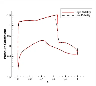
Figure 4.8 A comparison of the pressure distribution obtained by the high and low-fidelity models atM∞ = 0.734. . . 32
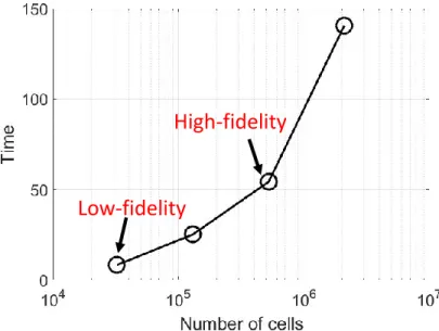
Figure 4.9 Variation of the simulation time with respect to the grid size for the grid study in Table 4.1. . . 33
Figure 4.10 Results of Strategy 1 showing the Pareto fronts obtained in at several iterations. . . 35
Figure 4.11 The final Pareto front of Strategy 1 with high-fidelity valiation samples. 35 Figure 4.12 Results of Strategy 2 showing the Pareto fronts obtained in at several iterations. . . 38
Figure 4.13 The final Pareto front of Strategy 2 with high-fidelity valiation samples. 38 Figure 4.14 Results of Strategy 3 showing the Pareto fronts obtained in at several iterations. . . 41
Figure 4.15 The final Pareto front of Strategy 3 with high-fidelity valiation samples. 41 Figure 4.16 Comparision of the final Pareto fronts obtained by the three strategies. 42 Figure 4.17 Designs selected along the final Pareto front of strategy 3 for visualization. 43 Figure 4.18 Airfoil shape of the designs selected from the final Pareto front of Strat-egy 3. . . 43
Figure 4.19 Pressure coefficient of designs selected from the final Pareto front of Strategy 3. . . 44
Figure 4.20 Pressure coefficient contours for design 1. . . 44
Figure 4.21 Pressure coefficient contours for design 2. . . 45
Figure 4.22 Pressure coefficient contours for design 3. . . 45
Figure 4.23 A comparison of the proposed multi-objective algorithm with the single-objective optimization using a scalarized single-objective function. . . 47
Figure 4.24 Results of Strategy 3 showing the Pareto fronts obtained with 500 initial sampling points. . . 49
Figure 4.25 Results of Strategy 3 showing the Pareto fronts obtained with 300 initial sampling points. . . 50 Figure 4.26 Results of Strategy 3 showing the Pareto fronts obtained with 100 initial
sampling points. . . 50 Figure 4.27 Results of Strategy 3 showing the Pareto fronts obtained with 100 initial
sampling points and 3 refinement points. . . 51 Figure 4.28 Results of Strategy 3 showing the Pareto fronts obtained with 1,600 and
ABSTRACT
Computationally efficient constrained multi-objective design optimization of transonic air-foils is considered. The proposed methodology focuses on fixed-lift design aimed at finding the best possible trade-offs between the conflicting objectives. The algorithm exploits the surrogate-based optimization principle, variable-fidelity computational fluid dynamics (CFD) models, as well as auxiliary approximation surrogates (here, using kriging). The kriging models constructed within a reduced design space. The optimization process has three major stages: (i) design space reduction which involves the identification of the extreme points of the Pareto front through single-objective optimization, (ii) construction of the kriging model and an ini-tial Pareto front generation using multi-objective evolutionary algorithm, and (iii) Pareto front refinement using co-kriging models. For the sake of computational efficiency, stages (i) and (ii) are realized at the level of low-fidelity CFD models. The proposed algorithm is applied to the multi-objective optimization of a transonic airfoil at a Mach number of 0.734 and a fixed lift coefficient of 0.824. The shape is parameterized with eight B-spline control points. The fluid flow is taken to be inviscid. The high-fidelity model solves the compressible Euler equations. The low-fidelity model is the same as the high-fidelity one, but with a coarser description and is much faster to execute. With the proposed approach, the entire Pareto front of the drag coefficient and the pitching moment coefficient is obtained using 100 low-fidelity samples and 3 high-fidelity model samples. This cost is not only considerably lower (up to two orders of magnitude) than the cost of direct high-fidelity model optimization using metaheuristics without design space reduction, but, more importantly, renders multi-objective optimization of transonic airfoil shapes computationally tractable, even at the level of accurate CFD models.
NOMENCLATURE
A Response correction matrix
AbaselineBaseline cross sectional area [m2]
Ac Cross sectional area of low-fidelity model [m2] Af Cross sectional area of high-fidelity model [m2] Amin Minimum cross sectional area [m2]
al Scalar terms of response correction matrixA ad Scalar terms of response correction matrixA
Cd Drag coefficient matrix of low-fidelity model
Cl Lift coefficient matrix of low-fidelity model Cd Drag coefficient [-]
Cd.c Drag coefficient of low-fidelity model [-] Cd.f Drag coefficient of high-fidelity model [-] Cl Lift coefficient [-]
Cl.c Lift coefficient of low-fidelity model [-] Cl.f Lift coefficient of high-fidelity model [-] Cm Pitching moment coefficient [-]
Cm.c Pitching moment coefficient of low-fidelity model [-] Cm.f Pitching moment coefficient of high-fidelity model [-] Cp Pressure coefficient [-]
D Response correction matrix
D Drag [N]
dl Scalar terms of response correction matrixA dd Scalar terms of response correction matrixA
Fl Lift coefficient matrix of high-fidelity model g(x) Inequality constraints
h(x) Equality constraints
H Scalar valued objective function
l Design variable lower bound
L Lift [N]
M∞ Mach number [-]
q Additive response correction
s Surrogate model
u Design variable upper bound
x Airfoil chord-wise location [m]
X B-spline control polygon coordinates
x Design variable
x∗ Optimized design variable
z Airfoil thickness [m]
CHAPTER 1. INTRODUCTION
1.1 Motivation and Challenges
The development of complex engineering systems requires us to deal with various conflict-ing objectives. For example, in the development of a cellphone we need to look into several objectives like cost, battery life, and aesthetics. Attaining the best values of all the objectives simultaneous may be an impossible task. In such cases, we want to know the optimal decisions that need to be taken in the presence of trade-offs between the competing objectives. Here, the task is to find a representative set of optimal solutions that satisfy the different objectives, the so-called Pareto-optimal set [2], which describes the trade-offs between these objectives. Pareto optimality, is a state of allocation of resources in which it is impossible to make any one individual better off without making at least one individual worse off [3].
We will explain the concept of Pareto optimality through an example. Let us assume that we are designing an aircraft where we want to obtain the trade-off between two objectives F = [F1 F2]T, where, for example, F1 is the cost and F2 is the range. Let us assume that
there are two design variables x = [x1 x2]T, where, for example, x1 is the wing span and
x2 is the wing thickness to chord ratio. Figure 1.1 shows the feasible design space and the
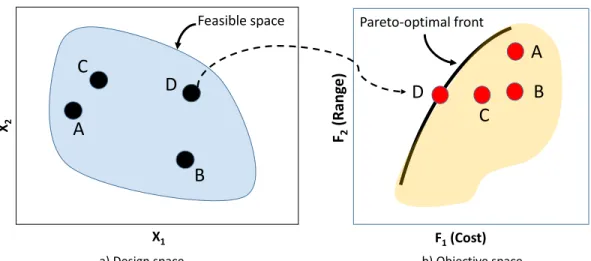
corresponding objective space. Consider designs A, B, C, and D. Out of these four designs, Design A gives the best range but at the same time it is the most expensive one. Similarly, Design B has a shorter range and is also very expensive. Design C, however, has the same range as B, but is much cheaper. Design D is cheaper than the other three designs, but has the same range as B and C. Moreover, Design D lies on the Pareto-optimal front, and represents the best design for the given values of the two objectives. In other words, it is not possible to find a design than has a longer range than Design D without increasing the cost.
A
A
C
D
B
B
C
D
F1(Cost) F2 (Rang e) X1 X2Feasible space Pareto-optimal front
a) Design space b) Objective space
Figure 1.1 Representation of the design space and the corresponding feasible objective space. Designs A, B, and C are non-optimal solutions. Design D lies on the Pareto-optimal front.
The above example explains how the trade-offs between conflicting objectives can be repre-sented within the design and objective spaces. A rudimentary approach to the simultaneous control of several objectives is a priori preference articulation (i.e., selection of the primary ob-jective such as cost), and handling the remaining obob-jectives by means of constraints of penalty functions. As a result, the problem can be solved as a single-objective one. However, in some situations it is of interest to gain more comprehensive information about the system at hand which may allow the designer to understand the characteristics of the possible trade-offs between conflicting objectives. In such a case, the entire Pareto front needs to be generated.
Multi-objective optimization [4] (MOO) (also called vector optimization or Pareto optimiza-tion) is used to obtain the trade-offs between competing objectives. There are various methods to perform MOO (Section 2 gives the background of MOO). A widely used approach involves the use of metaheuristic algorithms, such as genetic algorithms [5] (GAs), multi-objective evo-lutionary algorithm [6] (MOEAs), and particle swarm optimization [7] (PSO). Their primary advantage is the capability of generating the entire Pareto front representation in a single al-gorithm run. Unfortunately, metaheuristics are computationally intensive due to processing of large sets of candidate designs (population sizes of up to a few hundreds of individuals are not
F1(x
),
F2(x
)
Number of computational cells Number of computational cells
Time
(min
)
F1
F2
a) Objectives b) Simulation time
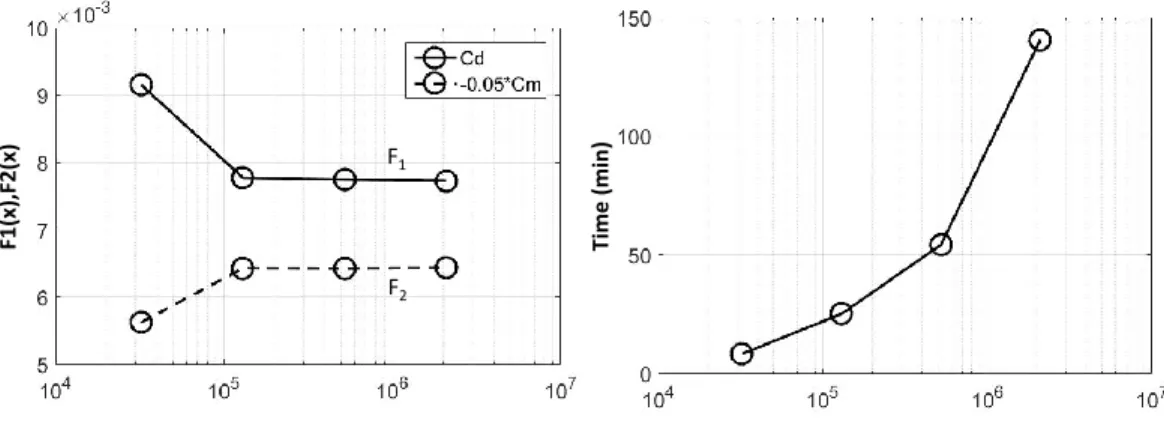
Figure 1.2 PDE simulations (such as computational fluid dynamics (CFD) simulations) need dense computational grids that require long CPU times (often on the order of days) on high performance computing clusters. The graph shows how the time and the objective function values of a 2D CFD simulation of transonic airfoil flow vary with the grid density.
uncommon). Consequently, metaheuristic algorithms are almost always limited to situations where the underlying computational model is very fast to execute and small design spaces.
High-fidelity partial differential equation (PDE) simulations are becoming increasingly im-portant in the design of complex multidisciplinary engineering systems. The reason behind this is that the physics governing these complex systems can be highly nonlinear. Moreover, nonlinear couplings between disciplines may exist. Furthermore, when considering unconven-tional systems, it may not be possible to rely on prior designs. High-fidelity PDE simulations are, therefore, essential in the development of many modern engineering systems, even at the initial conceptual stage, since lower fidelity methods may not be able to capture reliably the main characteristics to yield the best design. Unfortunately, high-fidelity PDE simulations are computationally expensive. For example, a single PDE simulation of the fluid flow past an aerodynamic surface, such as a typical transonic transport wing shape, can be on the order of one day when using high performance computing (HPC). Figure 1.2 gives an example for the two-dimensional inviscid transonic flow past a airfoil. The trends for a wing shape will be the same, but the simulation time will be an order of magnitude larger.
The key challenges with automated PDE-constrained MOO are as follows: (1) high com-putational cost of accurate PDE simulations, (2) large design space dimensionality and large parameter ranges, and (3) a large number of system evaluations required by conventional MOO techniques. The combination of (1) and (2) may yield design problems which are prohibitively expensive to solve using (3). Therefore, efficient methodologies are required to reduce the de-sign space, speed-up the simulations while still retaining a desired accuracy, and reduce the number of required system evaluations.
1.2 Research Objectives and Contributions
The overall objective of this research work is to investigate strategies to accelerate PDE-constrained MOO to enable fast iterative system design. To limit the scope, we focus the work on the design of airfoil shapes in transonic fluid flow. This design problem requires the computational fluid dynamics (CFD) simulations of the transonic fluid flow. Airfoil shapes are typically described using up to 15 parameters, and, in this work we parameterize the shapes with eight parameters. The objective is to generate the trade-offs of the airfoil characteristics. In particular, the trade-offs between the drag and pitching moment coefficients are generated at a fixed lift coefficient. Therefore, the MOO design problem considered in this work involves small-scale PDE simulations (on the order of 20 minutes on HPC) and a low-dimensional design space (8 parameters). Future work, will consider larger scales and higher dimensional problems. The MOO approach proposed in this work is as follows. We integrate fast physics-based surrogate models and design space reduction techniques to approximately identify the Pareto-optimal front, and, subsequently, refine the Pareto front using a limited number of computation-ally expensive system evaluations. To achieve this, we developed a computational framework which integrates variable-fidelity CFD models with numerical algorithms to perform the MOO. In particular, a critical step in the MOO process is to reduce the design space to enable the construction of an accurate approximation model (we use kriging interpolation [8]) with a lim-ited number of fast low-fidelity CFD models. The design space reduction is achieved through single-objective optimization of each objective separately. The kriging surrogate is then uti-lized to generate the initial approximate Pareto front using MOEA, which is computationally
efficient since the kriging surrogate is very fast. The approximate Pareto front is then refined by constructing a co-kriging model [8] on top of the initial kriging surrogate with a limited number of high-fidelity PDE simulations. To validate the approach, we perform MOO of the full design space and compare with the proposed approach.
1.3 Thesis Outline
The thesis is structured as follows. Chapter 2 provides the background of MOO, MOO algorithms, and MOO approaches used in aerodynamic design. The proposed MOO algorithm is described in Chapter 3. The results of the numerical application is given in Chapter 4. Chapter 5 concludes the thesis.
CHAPTER 2. BACKGROUND
2.1 Definition and Formulation of Multi-Objective Optimization
The process of optimizing systematically and simultaneously a collection of objective func-tions is called multi-objective optimization (MOO) (also called vector optimization, Pareto optimization, or multi-criteria optimization) [2]. MOO is an area of multiple criteria decision making, that deals with mathematical optimization problems involving more than one objec-tive function to be optimized simultaneously [4]. It has been applied in many fields of science, including engineering, economics and logistics where optimal decisions need to be taken in the presence of trade-offs between two or more conflicting objectives. Some of the few examples of multi-objective optimization problems involving two or three objectives are minimizing cost while maximizing comfort while buying a car, and maximizing performance whilst minimizing fuel consumption and emission of pollutants of a vehicle. Typically, the case of competitive objectives is the most interesting in the research field of MOP, because the choice of an “ac-ceptable” or “best” solution relies on the trade-offs of the objective functions, which ultimately depends on human preferences and decisions [9].
MOO can be described in mathematical terms as follows [2,3,4]
min(F1(x), F2(x), . . . , Fk(x)) (2.1)
subject togj(x)≤0, j = 1,2, . . . , m, (2.2)
hl(x) = 0, l= 1,2, . . . , e, (2.3)
where k is the number of objective functions, m is the number of inequality constraints, and e is the number of equality constraints. x ∈ En is a vector of design variables (also called decision variables), where n is the number of independent variablesxi. F(x) ∈Ek is a vector
of objective functions Fi(x) : En → E1. Fi(x) are also called objectives, criteria, payoff
functions, cost functions, or value functions. The feasible design space X (often called the feasible decision space or constraint set) is defined as the set {x|gj(x) ≤ 0, j=1 ,2,...,m; and hi(x) = 0, i= 1,2, ..., e}. The feasible criterion spaceZ (also called the feasible cost space or
the attainable set) is defined as the set{F(x)|x∈X}.
Unlike single-objective optimization, a solution to a multi-objective problem is more of a concept than a definition. Typically, there is no single global solution, rather we may need to determine a set of points that all fit a predetermined definition for an optimum. The main concept in defining an optimal point is that of Pareto optimality [10]. All Pareto optimal points lie on the boundary of the feasible criterion space Z [11]. Often, algorithms provide solutions that may not be Pareto optimal but may satisfy other criteria, making them significant for practical applications. All Pareto optimal points may be categorized as being either proper or improper. The idea of proper Pareto optimality and its relevance to certain algorithms is discussed by [12, 13]. It is defined as follows: Properly Pareto Optimal: A point, x ∈ X, is properly Pareto optimal (in the sense of [12]) if it is Pareto optimal and there is some real numberM ≥0 such that for eachFi(x) and eachx∈Xsatisfying Fi(x)< Fi(x?), there exists
at least oneFj(x) such that Fj(x?)< Fj(x) and (Fi(x?)−Fi(x))/(Fj(x)−Fj(x?))≤M. The
quotient is referred to as a trade-off, and it represents the increment in objective function j resulting from a decrement in objective function i. As required by the definition the trade-off between each function and at least one other function be bounded in order for a point to be properly Pareto optimal. For any given problem, there may be an infinite number of Pareto optimal points constituting the Pareto optimal set.
2.2 Multi-Objective Optimization Strategies and Algorithms
Several approaches and algorithms to solve MOO problems have been developed. The following is a brief description of several MOO approaches.
2.2.1 Single-Objective Optimization using a Scalarized Objective Function One way of solving the MOO problem is to scalarize the objectives and solve using single-objective optimization algorithms. The weighted sum method (WSM) is one way to scalarize the objectives. WSM transforms multiple objectives into an aggregated objective function by multiplying each objective function by a weighting factor and summing up all weighted objective functions as follows [14]
Jweighted sum =w1J1+w2J2+· · ·+wmJm, (2.4)
where wi, i = 1, . . . , m, is a weighting factor for the ith objective function. The weight
of an objective is chosen in proportion to the relative importance of the objective. The main disadvantage of this method is it is difficult to set the weight vectors to obtain a Pareto-optimal solution in a desired region in the objective space. Also it cannot find certain Pareto-optimal solutions in the case of a nonconvex objective space.
2.2.2 Evolutionary Algorithms
The term evolutionary algorithm (EA) stands for a class of stochastic optimization methods that simulate the process of natural evolution [6]. EAs have proven themselves as a general, robust and powerful search mechanism [15]. EAs seem to be especially suited to MOO because they are able to capture multiple Pareto-optimal solutions in a single simulation run and may exploit similarities of solutions by recombination. EAs operate on a set of candidate solution and use strong simplifications to subsequently modify the two basic principles of evolution: selection and variation. By ‘selection’ we mean the competition for resources among living beings. Some may be better than others and are more likely to survive and to reproduce their genetic information. In EAs, natural selection is simulated by a stochastic selection process. Each solution reproduces a certain number of time depending on their quality, which is assessed by evaluating the individuals and assigning them scalar fitness values. The other principle, ‘variation’, imitates natural capability of creating new living beings by means of recombination and mutation. According to some researchers multi-objective search and optimization might be a problem area where EAs do better than other blind search strategies [16]. Schaffer [17,
18] performed the first studies on evolutionary MOO in the mid-1980s. This multi-objective evolutionary algorithm (MOEA) approach was later used in various field pertaining to multi-objective problems [19]. The main objectives of MOEAs are [6]: (a) the distance of the resulting non-dominated front to the Pareto-optimal front should be minimized, (b) a good (in most cases uniform) distribution of the solutions found is desirable, and (c) the spread of the obtained non-dominated front should be maximized, i.e., for each objective a wide range of values should be covered by the non dominated solutions.
2.2.3 Genetic Algorithms
Genetic algorithms (GAs) are one of the approaches that can be used to solve MOO prob-lems directly. Holland [5] introduced GAs in 1975. Kocer [20] outlined a general GA and compared it with simulated annealing in its ability to minimize the cost of H-frame transmis-sion poles subjected to earthquake loading with discrete variables. Gen and Cheng [21] used GAs to treat problems related to industrial engineering, whereas Davis [22] provided a more general treatment. Because GAs do not require gradient information, they can be effective regardless of the nature of the objective functions and constraints. They combine the use of random numbers and information from previous iterations to evaluate and improve a popula-tion of points (a group of potential solupopula-tions) rather than a single point at a time. GAs are global optimization techniques, which means they may converge to the global solution rather than to a local solution. However, it is not true when working with MOO, which usually entails a set of solution points. Mathematically, we cannot have a single global solution to a MOO problem. The GA methods involve global optimization, i.e, they determine solutions that are globally Pareto optimal, not just locally Pareto optimal. Schaffer [18] presents one of the first treatments of multi-objective GAs, although he only considers unconstrained problems. Schaf-fer’s approach, which is also called the vector evaluated genetic algorithm (VEGA), involves producing smaller subsets of the original population, or sub-populations, within a given gen-eration. Pareto optimality as a concept is not embedded in the fundamentals of GAs. It has no correlation to the natural origins of genetic methods and hence it is possible with certain multi-objective GAs that a Pareto optimal solution may be born and then die out.
2.2.4 Particle Swarm Optimization
Particle Swarm Optimization (PSO) [7], another type of EA, simulates the movements of a flock of birds which aim to find food. The relative simplicity of PSO, and the fact that it is a population-based technique, have made it a natural candidate to be extended for MOO. Moore and Chapman proposed the first extension of the PSO strategy for solving multi-objective prob-lems in an unpublished manuscript from 1999 [23]. There was great interest among researchers to extend PSO after this early attempt. The next proposal was not published until 2002. The main issues about extending PSO to MOO are discussed in [24]. In order to apply the PSO strategy for solving MOO problems, the original PSO scheme has to be modified. Reyes-Sierra and Coello [25] present a comprehensive review of the various multi-objective particle swarm optimization (MOPSO).
2.3 Applications of Multi-Objective Optimization in Aerodynamic Design
Shape optimization is an important part of the design of aerodynamic components such as aircraft wings and turbine blades [26, 27]. Nowadays, the use of high-fidelity computational fluid dynamic (CFD) simulations is widespread in aerodynamic design. While searching for an improved design using CFD-based parameter sweeps and engineering experience is still a com-mon practice, design automation using numerical optimization techniques is becoming more and more popular [28,29]. Various methods and algorithms are available, from conventional, gradient-based algorithms [30], including those utilizing cheap adjoint sensitivities [31, 32], to the more and more popular surrogate-based optimization techniques [33, 34, 35] that of-fer efficient global optimization, and substantial reduction of the design cost as compared to traditional methods [36].
Aerodynamic design is inherently a multi-objective problem. In many cases, a primary objective (e.g., drag coefficient minimization) may be selected through a priori preference ar-ticulation, whereas the others (e.g., lift coefficient) can be handled through design constraints. This allows for solving the problem as a single-objective one. Sometimes, however, this is nei-ther possible nor convenient, e.g., when gaining knowledge about possible trade-offs between
competing objectives (example drag coefficient and pitching moment coefficient) is important. In those situations, solving a genuine MOO is necessary.
The following are just a few examples from the literature where MOO is used in aero-dynamic design. Shijun [37] uses the Davidon-Fletcher-Powell variable metric method as the multi-objective optimizer, and the Golden Section method for one-dimensional search, to max-imize flutter speed by tailoring the fiber orientations of the skin and spar web laminates of an aircraft wing. Wesley [38] uses a GA with discrete design variable to construct an object-oriented multi-disciplinary aerodynamic optimization (MDAO) tool. The MDAO tool and high-fidelity structural analysis is used to minimize the structural weight while maintaining desired flutter speeds of an X-56A aircraft. Kai [39] presented a novel multidisciplinary frame-work for performing multi-objective shape optimization of a flexible wing structure. Using a multidisciplinary algorithm both aerodynamic shape and structural topology are optimized concurrently using gradient based optimization. Gaetan [40] uses the weighted sum method and a gradient-based search algorithm to perform an multi-objective aero-structural optimization. Ekhlas [41] uses multi-objective evolutionary algorithm (MOEA) for optimum aerodynamic design of horizontal-axis wind turbines (HAWT). Using the evolutionary method of combined GA and with different airfoil profiles technique, turbine aerodynamic performance is optimized. Hanafy [42] uses strength Pareto evolutionary algorithm (SPEA) based approach for designing an integrated fuzzy guidance law. Mukesha [43] uses PSO and GA to solve an aerodynamic shape optimization problem concerning NACA 0012 airfoil using 12 design variables. Results show that the PSO scheme is more effective in finding the optimum solution among the various possible solutions. Overall, based on this brief literature survey, it seems that for aircraft and aerodynamic design, the weighted sum method and GAs are generally used for MOO. Moreover, in these works the high-fidelity model is utilized directly in the MOO process.
CHAPTER 3. MULTI-OBJECTIVE OPTIMIZATION METHODOLOGY
In this section, we define multi-objective aerodynamic design problem, and describe each step of the multi-objective optimization (MOO) algorithm proposed in this work. In particu-lar, we describe the variable-fidelity computational fluid dynamics (CFD) modeling and space mapping correction, design space reduction technique, and the kriging and co-kriging surrogate model construction. The utilization of the MOO algorithm is demonstrated in Chapter 4 using an example of transonic airfoil shape design.
3.1 Multi-Objective Aerodynamic Design Formulation
We will denote byxthe vector of design variables which are typically the geometry parame-terization coefficients of the aerodynamic surface of interest. Also, letf(x) = [f1(x) f2(x). . .
fk(x)]T be a vector ofkhigh-fidelity CFD model responses. Examples of responses include the
airfoil section drag coefficient f1(x) = Cd.f, and the section lift coefficient f2(x) = Cl.f. Let Fk(x), k= 1, . . . , Nobj, be the kth design objective. A typical performance objective would be
to minimize the drag coefficient (Cd.f), in which caseFk(x) =Cd.f. Another objective would
be to minimize the pitching moment coefficient (Cm.f), in which case Fk(x) =Cm.f.
A comparison of the design solutions in a multi-objective setting is performed using a Pareto dominance relation. It is necessary because if Nobj > 1, then any two designs x(1) and x(2)
for which Fk(x(1)) < Fk(x(2)) and Fl(x(2)) < Fl(x(1)) for at least one pair k 6= l, are not
commensurable, i.e., none is better than the other in the multi-objective sense. We define Pareto dominance relation 6 (see, e.g., Fonseca [2]), saying that for the two designs x and y,
we havex6 y(xdominates overy) ifFk(x)≤Fk(y) for allk= 1, . . . , Nobj, andFk(x)< Fk(y)
front (of Pareto-optimal set) XP of the design space X, such that for any x ∈ XP, there is
no y ∈ X for which y 6 x (Fonseca [2]). In practice, the Pareto front gives us information
about the best possible trade-offs between the competing objectives, such as the minimum drag and pitching moment coefficients for a given value of the lift coefficient. Having a reasonable representation of the Pareto front is therefore indispensable in making various design decisions. In practice, the identification of a set of alternative Pareto-optimal solutions needs to be followed by a decision making process, so that a single final design is selected for prototyping and subsequent manufacturing. This is done based on given preferences concerning, among others, importance of particular objectives. In this work, we only focus on the methodology for obtaining the Pareto front itself. The decision making process is beyond the scope of this work.
3.2 Optimization Algorithm
As mentioned in the introduction, a fundamental bottleneck of PDE-constrained optimiza-tion of complex systems is the high cost of the accurate, high-fidelity models, which is especially challenging in MOO. Therefore, for the sake of computational efficiency, the MOO procedure presented here exploits, apart from the original, high-fidelity model f, its low-fidelity model counterpart c. In this work, the low-fidelity model is based on coarse-discretization CFD sim-ulations (its detailed setup is discussed in Chapter 4, which allows for a fast evaluation at the cost of some accuracy degradation. A design speedup is achieved by performing most of the operations at the level of the low-fidelity model; however, high-fidelity simulations are also executed in order to yield a Pareto set that is sufficiently accurate.
We present the entire MOO flow now, and then discuss each step in the following subsec-tions. The proposed MOO algorithm is as follows:
1. This step is optional. Correct the low-fidelity model c using output space mapping to construct a surrogate models0. If the correction is not performed, thens0=c;
2. Perform design space reduction usings0;
4. Construct a kriging surrogatesKR based on the data from Step 3;
5. Obtain an approximate Pareto set representation by optimizingsKR using MOEA;
6. Evaluate the high-fidelity model f along the Pareto front; 7. Construct/update the co-kriging surrogatesCO;
8. Update Pareto set by optimizing sCO using MOEA;
9. If termination condition is not satisfied go to Step 6; else END Comments on each step in the above MOO algorithm:
Step 1: Searching for a Pareto front in a large design space using expensive high-fidelity PDE
simulations is not practical, and, hence, a fast surrogate model will speed up the process. For the sake of reliability, output space mapping (Section3.3) can be used to correct high-fidelity CFD models. However, this step may be skipped since the algorithm uses kriging (Step 4) and co-kriging (Step 7) to generate the Pareto front. These data-driven surrogates can provide the necessary alignment of the low-fidelity model with the high-fidelity one.
Step 2: Setting up an accurate data-driven surrogate (Step 4) can be very expensive to do in a
large design space, i.e., wide parameter ranges, with multiple design variables. Hence, reducing the design space is a critical part of the propose MOO algorithm. With a smaller design space (in terms of reduced design variable parameter ranges, as well as reduced dimensionality), the kriging (Step 4) and co-kriging (Step 7) models can be set up accurately using few model evaluations. The design space reduction methodology is described in Section3.4.
Step 3: Latin Hypercube Sampling (LHS) [44] is used to select the shapes within the reduced
design space for the kriging model construction. The LHS sampling is described in Section3.5.
Step 4: Using the sampled data from Step 3, a kriging interpolation model is constructed.
Section3.5 describes the surrogate model construction.
Step 5: A multi-objective evolutionary algorithm (MOEA) is run using the kriging model
(from Step 4) to generate an initial approximation of the Pareto set. Note, however, the Pareto set obtained is not accurate to the high-fidelity level as we obtain it using the approximate
surrogate which is based on the low-fidelity model. Here, we use a standard MOEA with fit-ness sharing, Pareto-dominance tournament selection, and mating restrictions [2]. The main changes (compared to single-objective evolutionary algorithms) are the mechanisms that push the solutions towards the Pareto front (here, realized through Pareto-dominance-based fitness function as well as the aforementioned selection procedure) and spread the solutions along the front (here, realized using fitness sharing and mating restrictions). The algorithm is modified in order to handle nonlinear constraints. The modification include: (i) initialization proce-dure that only generated feasible individuals, and (ii) crossover and mutation proceproce-dures that maintain feasibility of individuals.
Step 6 and 7: Designs are sampled uniformly along the Pareto front predicted by the initial
kriging model optimization. Those designs are then evaluated using the high-fidelity model. A co-kriging model is then constructed (or updated) using all the high-fidelity model data accumulated during the algorithm run. Only a few high-fidelity model evaluations are used per iteration. The co-kriging model construction is discussed in Section 3.6.
Step 8: The co-kriging model is used to refine the Pareto front using the MOEA. In practice,
just a few iterations are sufficient for convergence. If the alignment between these samples and the surrogate ones is sufficient, the algorithm is terminated. The convergence condition is based on the distance between the predicted front and the high-fidelity verification samples (distance measured in the feature space). In the case of the presented aerodynamic design problems, the threshold is set to 2 drag counts (one drag count is defined as ∆Cd = 0.0001)).
3.3 Variable-Fidelity Surrogate Model
The main optimization engine utilized here for Pareto front identification is MOEA [45]. Due to excessive computational cost of population-based procedures such as MOEAs, it is not practical to apply evolutionary search directly at the level of the expensive PDE simulation model f(x) = [Cd.f(x) Cm.f(x)]T (the lift coefficient Cl.f(x) is kept constant by implicitly
varying the angle of attack). Instead, we exploit a faster representation of the high-fidelity model, which is a surrogate constructed as follows. Let c(x) = [Cd.c(x)Cm.c(x)]T denote the
obtained by the low-fidelity CFD model (the low-fidelity lift coefficientCl.c(x) is kept constant
by implicitly varying the angle of attack). The description and setup of the high- and low-fidelity models has been described in Chapter 4. The output space mapping (OSM) surrogate model s in Step 1 of the MOO algorithm (Section3.2) is constructed as follows.
Enhancement of the low-fidelity model. In this step, the initial surrogate model s0(x)
is obtained by applying a parameterized output space mapping (OSM) [46, 47]. OSM uses correction terms that are directly applied to the response components Cd.c(x) andCm.c(x) of
the low-fidelity model (drag coefficient and pitching moment, respectively). The aerodynamic surrogate model is defined as [47]
s0(x) =A(x)◦c(x) +D(x), (3.1)
where ◦ denotes component-wise multiplication, and A(x) and D(x) are multiplicative and additive correction terms. Both terms are design-variable-dependent and take the form of
A(x) = [ad.0+ [ad.1ad.2....ad.n]·(x−x0) am.0+ [am.1am.2....am.n]·(x−x0)]T, (3.2)
D(x) = [dd.0+ [dd.1dd.2....dd.n]·(x−x0) dm.0+ [dm.1dm.2....dm.n]·(x−x0)]T, (3.3)
wherex0 is the center of the design space. Response correction parametersA(x) andD(x) are obtained as
[A,D] = arg min
[ ¯A,D¯]
N
X
k=1
||f(xk)−( ¯A(xk)◦c(xk) + ¯D(xk))||2 (3.4) i.e., the response scaling is supposed to (globally) improve the matching for all training points xk,k= 1, . . . , N.
In this work, we use a training set consisting of (i) factorial design with 2n+ 1 training points (nbeing the number of design variables) allocated at the center of the design space x0 = (l+ u)/2 (l andu being the lower and upper bound for the design variables, respectively), and the centers of its faces, i.e., points with all coordinates but one equal to those of x0, and
also referred to as the star distribution [36], (ii) additional 10 points allocated using the Latin Hypercube Sampling [44]. The only formal requirement for the necessary number of samples is that it is larger than the number of model coefficients to be identified.
The correction parameters A and D can be calculated analytically as follows [47]
ad.0 ad.1 .. . ad.n dd.0 .. . dd.n = (CTdCd)−1CTdFd am.0 am.1 .. . am.n dm.0 .. . dm.n = (CTmCm)−1CTmFm (3.5) where Cd= Cd.c(x1) Cd.c(x1)·(x11−x01) . . . Cd.c(x1).(x1n−x0n) 1 (x11−x01) . . . (x1n−x0n) Cd.c(x2) Cd.c(x2).(x21−x01) . . . Cd.c(x2)·(x2n−x0n) 1 (x11−x01) . . . (x1n−x0n) .. . ... . .. ... ... ... ... ... Cd.c(xN) Cd.c(xN)·(xN1 −x01) . . . Cd.c(xN)·(xNn −x0n) 1 (x11−x01) . . . (x1n−x0n) (3.6) F= Cm.f(x1) Cm.f(x2) . . . Cm.f(xN) T (3.7) which is a least-square optimal solution to the linear regression problems [ad.0 ad.1 . . .ad.n dd.0
dd.1 . . . dd.n]TCd = Fdand [am.0 am.1 . . .am.n dm.0 dm.1 . . . dm.n]TCm =Fm, equivalent to
(3.4). Note that the matrices CTl Cl and CTdCd are non-singular for N > n+ 1, which is the
case for our choice of the training set.
The enhancement of the low-fidelity model using OSM can be skipped since it can be costly. The data-driven surrogates (Steps 4 and 7) may take care of the low-fidelity model alignment with the high-fidelity one. In this case, the surrogate model is simply
3.4 Design Space Reduction
The MOO algorithm proposed in this work is heavily based on data-driven surrogate models. Therefore, it is of primary importance to ensure that the training data for creating the surrogate models can be acquired in a reasonable timeframe, even if the dimensionality of the design space is relatively large (say, more than 10 parameters). Here, similar as done in Koziel et al. [1], we carry out an initial design space reduction in order to identify the sub-region of the search space that contains the Pareto-optimal solutions. This region is usually a very small fraction of the original space. It is partially because the bounds for each geometry parameter are defined rather wide to ensure that the desired solutions are located within these prescribed limits. Nonetheless, setting up a data-driven surrogate in a large solution space may be impractical. However, the bounds of the design variables can be conveniently minimized using single-objective optimization runs with respect to each design goal. The result of those optimization runs should give us an approximation of where the extreme points of the Pareto-optimal set lie.
Considerlandu as the initial lower and upper bounds, respectively, for the design variable vectorx. Single-objective optimization of each objective Fk yield the approximate location of
the extreme points xcof the Pareto-optimal set, and can be found as
x∗c(k)=arg min
l≤x≤uFk(s0(x)) (3.9)
where k= 1, . . . , Nobj. The boundaries of the reduced design space can be then defined as l∗
= min{x∗c(1),....,x ∗(Nobj) c } and u∗ = max{x ∗(1) c ,..., x ∗(Nobj)
c }. The concept of the search space
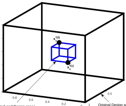
reduction is illustrated in Fig. 3.1. The reduced space is usually orders of magnitude (volume-wise) smaller than the initial one, which makes the generation of an accurate data-driven model possible at a reasonably low computational cost. Although some of the Pareto optimal solutions might fall outside the reduced design space, a majority of them are normally accounted for assuming that the objectives are continuous functions of the design variables and the Pareto front is a connected set.
0 1 0.2 1 0.4 0.8 0.6 0.6 0.8 0.4 1 0.2 0.5 0 0
Reduced Design space Original Design space
xc*(1)
xc*(2)
Figure 3.1 An illustration of the design space reduction technique using single-objective op-timization runs (Koziel et al. [1]). The illustration assumes a three-dimensional design space and two design objectives.
3.5 Kriging Surrogate Construction
A kriging interpolation surrogate model is constructed in Step 4 of the MOO algorithm presented in Section 3.2. An outline of the process of constructing the surrogate is shown in Fig. 3.2 which involves performing design of experiments (DOE), data acquisition, model fitting, and model validation. Each step in the process is described in detail here below.
3.5.1 Design of Experiments
DOE is a technique to distribute sample points within the design space [35]. In this work, we use Latin Hypercube Sampling (LHS) [35]. LHS is a statistical method for generating a sample of a given parameter value from a multidimensional distribution, and ensures that each probability distribution in the model is evenly sampled. The idea of LHS is to use bins to sample the points along each design variable dimension. For example, as shown in Fig. 3.3, if
Design of Experiments
Model Data Acquisition
Kriging Interpolation
Model Validation
Figure 3.2 Flowchart describing the data-driven surrogate modelling process
the range of each design variable is split into 20 bins, for the two-dimensional case, there are 202 cells in the design space. The samples are allocated randomly so that for each dimension bin there is only one sample inside.
3.5.2 Kriging Interpolation
A kriging [8] interpolation model is utilized in this work to yield an initial approximation of the Pareto set. It is also the core of the co-kriging approach described in Section3.6. This section briefly provides background information on kriging interpolation. A detailed survey can be found in the literature [48,49].
Let XB = {x1,x2, ...,xN} be a training set, and letf(XB.KR) be the corresponding set of
high-fidelity model responses. The aim of kriging interpolation is to fit a regression function on the training nodes and build a Gaussian Process (GP) through the residuals [8]. The regression function sKR(x) captures highest variance in the training samples while the GP covers the
Figure 3.3 Latin Hypercube Sampling Illustration
details related to the interpolation accuracy. This is provided by a kriging interpolant denoted as
SKR(x) =Mα+r(x)·Ψ−1·(f(XB.KR)−Fα), (3.10)
whereMandFare model matrices of the test nodexand the base setXB.KR, respectively.
The vector α is a regression function coefficient of the form
α= (XB.KR0 Ψ−1XB.KR)−1XB.KRΨ−1(f(XB.KR)) (3.11)
while r(x) = (Ψ(x,x1KR), ...,Ψ(x,xNKR
KR )) is an 1×NKR vector of correlations between the
point xand the base setXB.KR, and Ψis aNKR×NKR correlation matrix given by
Ψ(x1KR,x1KR) . . . Ψ(x1KR,xNKR KR ) .. . . .. ... Ψ(xNKR KR ,x1KR) . . . Ψ(x NKR KR ,x NKR KR ) (3.12)
The kriging interpolation model is capable to predict the approximation error at any location in the solution space. The error is zero at the training nodes, which is because kriging is an interpolative model. The regression function actually operates as the mean of the GP, thus the predictions situated too far from existing training nodes (e.g., outside the sampled region)
will revert to the average values. The nature of the response is usually unknown so that a constant regression function (referred to as ordinary kriging) is often utilized. One should note that in such cases, kriging is solely an interpolation method without the possibility of response extrapolation. The choice of the proper correlation function is important in order to create an accurate kriging surrogate. A widely used class of correlation functions dependent only on the distance between any two points (here xand x’) is defined by:
Ψ(x,x’) =exp X k=1,...,n −θk|xk−xk|p , (3.13)
where the parameter p determines the prediction smoothness, whileθk,k = 1, . . . , n, denotes
the influence sphere of a node on its neighbors in each dimension [50]. This is helpful for identification of relevant variables as it describes the linearity of the response. Usually, p
is constant while the parameters θk are determined using Maximum Likelihood Estimation
(MLE) [51], where the negative concentrated log-likelihood is minimized using
ln(L)≈ −NKR/2×ln(σ2)−1/2 ln(|Ψ|), (3.14)
and
σ2= (f(XB.KR)−Fα)0Ψ−1(f(XB.KR)−Fα)/NKR. (3.15)
Usually,p= 2 is selected (also known as the Gaussian correlation function), which is suitable for many problems. In the case of sharp responses, selecting p= 1 (which corresponds to the exponential correlation function) is normally more suitable. Finally, because no extrapolation capabilities are required, the regression function is set to be constant, i.e., F= [1 1 . . .1]T and M= (1).
3.5.3 Model Validation
Model validation is needed to check the quality of the surrogate model constructed in the data fitting process. Apart from the sampled set of designs that are used to construct the kriging model, a randomly selected subset is set aside for model validation purposes. The main purpose of these sets is to allow us evaluate the difference between the true model and the
kriging model values at the specified test sites. In this work, we use the root mean square error (RMSE) metric [35]. We take a set of data of the size nt and a set of predictions at those
locations and calculate the RMSE as
RM SE= s Pnt i=0(y(i)−yˆ(i))2 nt (3.16)
where nt is the size of test data, y(i) is the true data and ˆy(i) is the predicted function value
by the surrogate. Generally, we want the RMSE metric to be as small as possible. A kriging model with a RMSE value less than 2% can be considered as a reasonably good model, and can be used reliably within a surrogate-based optimization process [35].
3.6 Co-kriging Surrogate Construction
In this work, combining variable-fidelity CFD simulation data into a single surrogate model is of primary importance for reducing the cost of the Pareto-optimal set identification. For that purpose, we follow the work of Koziel et al. [52] and use co-kriging [8]. Co-kriging is an extension of kriging which exploits correlations between the models of various fidelities. This results in a considerable enhancement of the surrogate prediction accuracy even if the number of high-fidelity data samples is very small compared to what is normally required by single-level (in particular, conventional kriging) modeling. Here, the autoregressive co-kriging model of Kennedy et al. [53] is adopted.
The generation of the co-kriging model is carried out through a sequential construction of two kriging models: the first model sKRc dervied from the original surrogate training samples
(XB.KRc,c(XB.KRc)), and the second sKRd model generated on the residuals of the high- and
low-fidelity samples (XB.KRf, sd), where sd=f(XB.KRf)−ρc(XB.KRf). The parameter ρis a
part of MLE of the second model. Ifc(XB.KRf) is not available, it can be approximated by the
first model, i.e., asc(XB.KRf)≈sKRc(XB.KRf). One should emphasize that the configuration
(specifically, the choice of the correlation function, regression function, and so forth) of both models can be adjusted separately for the low-fidelity datacand the residuals sd, respectively.
F= [1 1 . . . 1]T and M= (1). The final co-kriging model sCO(x) is defined similarly as
in (3.10), i.e.,
sCO(x) =Mα+r(x)·Ψ−1·(Sd−Fα), (3.17)
where the block matricesM,F,r(x), and Ψof (3.14) can be written as a function of the two underlying kriging models sKRc and sKRd as
r(x) = [ρ·σc2·rc(x) ρ2·σ2c·rc(x, XB.KRf) +σ 2 d·rd(x)], Ψ = σ2cΨc ρ·σ2c·Ψc(XB.KRc, XB.KRf) 0 ρ2·σc2·Ψc(XB.KRf, XB.KRf) +σ 2 d·Ψd , F= Fc 0 ρ·Fd Fd , and M= [ρ·Mc Md].
CHAPTER 4. NUMERICAL APPLICATIONS
In this chapter, we demonstrate the multi-objective optimization (MOO) algorithm of Sec-tion3.2on the design of aerodynamic surfaces. The case considers transonic airfoil shapes with eight design variables, and two conflicting objectives. In particular, we generate the trade-offs for the drag and pitching moment coefficients at a constant lift coefficient. The chapter is organized as follows. The problem is described in detail first. Three variations of the proposed MOO algorithm (which we call Strategies 1, 2, and 3) are applied to the design problem and the results presented. The chapter ends with a comparison of the strategies, and a parametric study of the third strategy.
4.1 Problem Description
Here, we give the details of the following: formulation of the problem, the design variable parameterization, training data sampling, variable-fidelity computational fluid dynamics (CFD) modeling, and an outline of the investigations with the three strategies.
4.1.1 Formulation of the MOO Problem
We consider multi-objective airfoil design in transonic flow at fixed lift. In particular, the free-stream Mach number is set to M∞ = 0.734, and the lift coefficient is fixed at Cl.f(x) =
0.824, where the subscriptf refers to the high-fidelity model, andxis the design variable vector with a lower bound l and an upper bound u. The first objective is F1(x) = Cd.f(x), where Cd.f is the high-fidelity drag coefficient. The second objective is F2(x) =Cm.f(x), whereCm.f
is the high-fidelity pitching moment coefficient. Both objectives are minimized. We impose a constraint on the cross-sectional area, i.e., we have A(x)≥ Abaseline, where A(x) the
cross-sectional area of a given design xnondimensionalized with the chord squared, and Abaseline is
a baseline reference value.
4.1.2 Design Space
We use the B-spline parameterization approach to describe the shape of the airfoil. The design variable vector is x =p, where p is a vector of the size m×1, with m being the total number of control parameters. The airfoil surfaces are written in parametric form as [54]
x(t) = n+1 X i=1 XiNi,k(t), z(t) = n+1 X i=1 ZiNi,k(t), (4.1)
where (x, z) are the Cartesian coordinates of the airfoil surface, Ni,k is the B-spline basis
function of orderk, (Xi, Zi) are the coordinates of the B-spline control polygon, andm=n+ 1
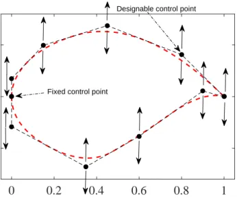
is the total number of control points. Note that the surface description with (4.1) is continuous. The control points are used as design variables and allowed only to move freely vertically as shown in Fig. 4.1. Thus, we have x = [Z1 Z2 . . . Zn+1]T and the corresponding Xi
coordinates are fixed during the optimization process. In this work, we use 8 design variables with 4 for each surface (as shown in Fig.4.1).
0 0.2 0.4 0.6 0.8 1
x
-0.05 0 0.05z
Designable control point
Fixed control point
Figure 4.1 Example B-spline parameterization of an airfoil. The designable control points are restricted to vertical movements only.
We use the RAE 2822 airfoil as a baseline. The shape is fitted to a B-spline curve by setting the x-locations of design variables as X = [Xu; Xl]T = [0.0 0.15 0.45 0.8; 0.0 0.35 0.6
0.9]T. After the fit, the baseline design variable vector is x0 = [xu; xl]T = [0.0175 0.04975
0.0688 0.0406; -0.0291 -0.0679 -0.03842 0.0054]T. The bounds of the design space are defined byl= (1−sign(x0)·0.15)◦x0 andu= (1 +sign(x0)·0.15)◦x0. Using the definition, the lower
and upper bounds on x0 are set as l = [0.0105 0.0414 0.0537 0.0200; -0.0369 -0.0808 -0.0666
-0.0265]T andu = [0.0231 0.0629 0.0889 0.0816; -0.0231 -0.0536 -0.0210 0.0140]T, respectively. The baseline reference cross-sectional area is ARAE2822= 0.0779.
4.1.3 Training Points
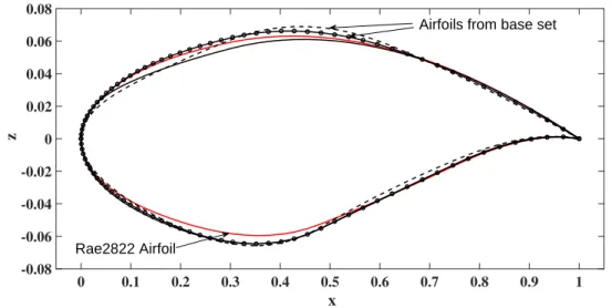
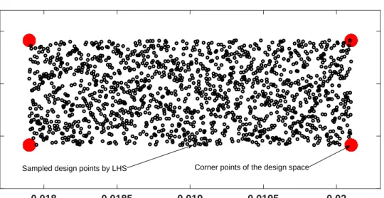
Sets of design points are generated around the baseline airfoil (the RAE 2822), within the upper and lower bounds, using Latin Hypercube Sampling (LHS) (see Section 3.5). Apart from LHS sampling, 256 corner points of the design space are generated and included in the set. Once the points are generated, each of them are checked for violation of area constraint and those infeasible are removed. An initial base set of 1,600 designs is used in all the strategies (this number is based on the mean square error and the values for each strategy are given in the results). Figure 4.2shows the baseline airfoil, as well as a few samples from the base set. Figure 4.3shows the design points (in black) for 2 of the control points.
0 0.1 0.2 0.3 0.4 0.5 0.6 0.7 0.8 0.9 1 x -0.08 -0.06 -0.04 -0.02 0 0.02 0.04 0.06 0.08 z Rae2822 Airfoil
Airfoils from base set
0.018 0.0185 0.019 0.0195 0.02 X1 (1st control point) 0.0423 0.04235 0.0424 0.04245 X2 (2nd control point)
Corner points of the design space Sampled design points by LHS
Figure 4.3 Example training points sampled using Latin Hypercube Sampling.
Output space mapping is utilized in Strategy 2 to setup the inital surrogate. In that case, a set of 30 points for the low- and high-fidelity simulations are generated within the given lower and upper bounds. Out of the 30 points, 2n+ 1 points are generated using a star distribution (these are at the centers of bounds and at the center, hence the name), and the rest are generated using LHS.
4.1.4 Computational Fluid Dynamics Modeling
The Stanford University Unstructured (SU2) computer code [55] is utilized for the fluid flow simulations. The steady compressible Euler equations are solved with an implicit density-based formulation. The convective fluxes are calculated using the second order Jameson-Schmidt-Turkel (JST) scheme [56]. Three multi-grid levels are used for solution acceleration. Asymptotic convergence to a steady state solution is obtained in each case. The flow solver convergence criterion is the one that occurs first of the two: (i) the change in the drag coefficient value over the last 100 iterations is less than 10−4, or (ii) a maximum number of iterations of 1,000.
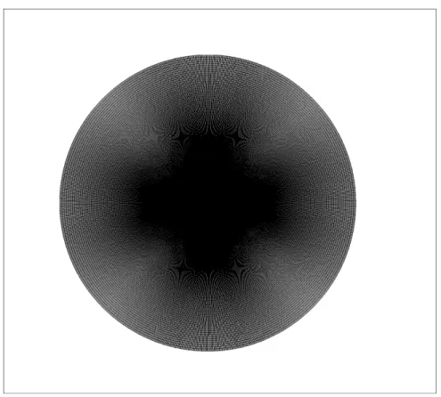
An O-type computational mesh is generated using Pointwise. The farfield boundary is set 55 chord lengths away from the airfoil surface. The mesh density is controlled by the number of
cells on the airfoil surface and the number of cells normal to the surface. Distance to the first grid point is 0.001c. The results of a grid convergence study, given in Table4.1, revealed that the 512×512 mesh (shown number 5 in the table) is required for convergence within 0.2 drag counts (1 drag count is ∆Cd= 10−4) when compared with the next mesh. The flow simulation
for Mesh 5 takes about 30 minutes. This time includes several simulations to obtain the desired lift coefficient by varying the angle of attack. Typically, 3 to 4 simulations are required.
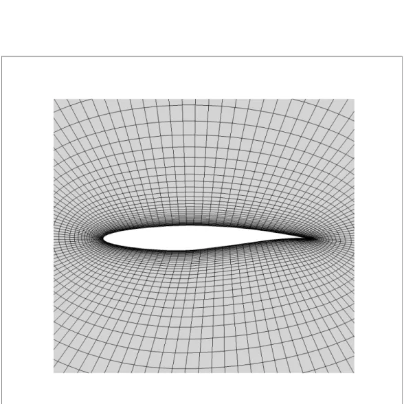
For the multi-objective optimization studies, Mesh 5 will be used as the high-fidelity modelf, and Mesh 3 as the low-fidelity modelc. Figures4.4,4.5, and4.6show the computational grids. For the low-fidelity model, the maximum number of solver iterations is set to 300. Figure
4.1.5 shows the solver convergence of the low-fidelity model. Consequently, the high-to-low
simulation time ratio is around 30 (see Fig. 4.9). A comparison of the pressure distributions, shown in Fig. 4.8, indicates that the low-fidelity model, in spite of being based on much coarser mesh and reduced flow solver iterations, captures the main features of the high-fidelity model pressure distribution quite well. The comparison indicates that the low-fidelity model may be a relatively good representation of the high-fidelity one. The biggest discrepancy in the distributions is around the shock on the upper surface, leading to an under estimation of both the drag and pitching moment coefficients (Table4.1). Note that the drag and pitching moment coefficients are presented in terms of counts. We define one drag count (d.c.) to be ∆Cd =
0.0001, and one pitching moment count (p.c.) to be ∆Cm = 0.00127.
4.1.5 Investigations
We solve the problem described in this section using three strategies. Each strategy uses the MOO algorithm in Section 3.2, but with different setup of the initial surrogate, as well as with and without the design space reduction step. We compare the strategies in terms of Pareto front findings and computational cost.
Figure 4.4 Visualization of the high-fidelity model computational mesh.
Table 4.1 Results of the grid convergence study at M∞= 0.734 and Cl= 0.824. Grid Size Cd Cm 64×64 0.0221 0.1384 128×128 0.0228 0.1439 256×256 0.0230 0.1448 512×512 0.0231 0.1450
0 50 100 150 200 250 300 −0.2 0 0.2 0.4 0.6 0.8 1 1.2 1.4 Solver Iterations C d ,C l ,C m C d C m Cl
Figure 4.7 Evolution of lift, drag and pitching moment coefficients obtained by the low fidelity model at M∞ = 0.734.
Figure 4.8 A comparison of the pressure distribution obtained by the high and low-fidelity models atM∞ = 0.734.
High-fidelity
Low-fidelity
Figure 4.9 Variation of the simulation time with respect to the grid size for the grid study in Table4.1.
4.2 Strategy 1
In Strategy 1, we follow the MOO algorithm in Section3.2, but we skip the Output Space Mapping correction and utilize the low-fidelity model, i.e., s0(x) = c(x). We also skip design
space reduction (step 2) and perform MOO on the original design space. Below, we outline the MOO algorithm, give results and summarize the computational cost.
4.2.1 MOO Algorithm
The steps of the MOO algorithm for Strategy 1 are as follows:
1. Sample the design space and acquire the low-fidelity model data withc; 2. Construct a kriging surrogatesKR based on the data from Step 1;
3. Obtain an approximate Pareto set representation by optimizingsKR using MOEA;
4. Evaluate the high-fidelity model f along the Pareto front; 5. Construct/update the co-kriging surrogatesCO;
6. Update Pareto set by optimizing sCO using MOEA;
7. If termination condition is not satisfied go to Step 5; else END
4.2.2 Results
The MOO algorithm was stopped after 7 iterations. Figure 4.10 shows the 1st, 3rd, 5th, and the 7th Pareto fronts. After the initial Pareto generation using the kriging model, 9 high-fidelity refinement samples are evaluated along the front. Subsequently, the co-kriging model is constructed and optimized using MOEA. This is repeated 7 times. Figure4.11shows the final Pareto and several high-fidelity model validation samples. It can be observed that the Pareto front predicted in the final iteration is close to the high fidelity verification samples. However, even after 7 iterations, the agreement between the predicted front and the verification samples is good except at its right-hand-side edge where the actual high-fidelity model samples exhibit higher pitching moments. Further iterations were performed, but it was found that the results did not improve much.
0 10 20 30 40 50 60 70 80 90 100 110 F1 (Drag Counts) 70 75 80 85 90 95 100 105 110
F2 (Pitching Moment Counts)
1st Pareto 3rd Pareto (green)
7th Pareto 5th Pareto (red)
Figure 4.10 Results of Strategy 1 showing the Pareto fronts obtained in at several iterations.
0 20 40 60 80 100 120 F1 (Drag Counts) 70 75 80 85 90 95 100 105 110
F2 (Pitching Moment Counts)
High-fidelity verification samples Final pareto after 7 iterations (Strategy 1)
4.2.3 Computational Cost
The overall computational cost of the multi-objective process in terms of number of evalu-ations is 1,600 (1,475 feasible points and 125 feasible corner points) low-fidelity model evalua-tions, and 63 high-fidelity model evaluations (9 each in 7 iterations of co-kriging-based Pareto front refinements). The cost of the kriging and co-kriging function evaluations in the MOEA process is ignored as the calculations are performed very quickly.
In terms of time, there is a significant advantage of the proposed method with variable-fidelity models compared to that of using the high-variable-fidelity directly. Each low-variable-fidelity model simulation is less than 1 min, and each high-fidelity model simulation is around 30 min. Hence, for 1,600 low-fidelity model simulations and 63 high-fidelity model simulations, the total time is around 3,490 minutes, or 2.4 days. However, the proposed method did not converge even after 9 iterations and hence the total time can be up to around 3 days. Using only the high-fidelity model, and assuming 1,663 samples are still needed, the total time would be around 34.6 days.
4.3 Strategy 2
Strategy 2 follows the MOO algorithm in Section 3.2 with the following modifications. We perform the OSM correction of the low-fidelity model (Step 1), but skip the design space reduction (Step 2) and perform MOO on the original design space.
4.3.1 Description
The steps of the MOO algorithm for Strategy 2 are as follows:
1. Correct the low-fidelity model c using output space mapping to construct a surrogate model s0;
2. Sample the design space and acquire the surrogate model data withs0;
3. Construct a kriging surrogatesKR based on the data from Step 3;
4. Obtain an approximate Pareto set representation by optimizingsKR using MOEA;
6. Construct/update the co-kriging surrogatesCO;
7. Update Pareto set by optimizing sCO using MOEA;
8. If termination condition is not satisfied go to Step 5; else END
4.3.2 Results
Figure 4.12 shows the results of the Strategy 2 iterations. In this case, three iterations of the MOO are enough to converge. Apart from the 1,600 points, extra 30 feasible points are generated to calculate to construct the initial surrogate s0. These points include 2n+ 1
corner points (wheren= 8 is the number of design variables) and the rest points are from LHS sampling (Section 4.1.3). While collecting points to calculate the OSM correction parameters, care is taken that the infeasible designs (the ones violating the area constraint) are removed. The 1,600 low-fidelity data samples are corrected to approximate it near to the high-fidelity model. Using these corrected set, the kriging model sKR is generated, which is subsequently
used to perform the MOEA and get the first Pareto front. Then, the Pareto is refined using 9 high-fidelity verification samples evaluated along the Pareto front to generate the co-kriging model sCO as described in Section 3.6 until convergence. It can be observed from Fig. 4.12
that the Pareto front predicted in the third iteration is converged within 1 d.c., i.e, after three iterations, the agreement between the predicted front and the refinement samples is withing 1 d.c.
4.3.3 Computational Cost
The overall computational cost of the MOO process in terms of number of evaluations are the initial 1,600 low-fidelity model evaluations, and 30 low- and high-fidelity model evaluations for OSM correction. Then 27 high fidelity model evaluations are used for the refinement phase (9 in each of the 3 iterations). The total time is 3,340 minutes, or 2.3 days.