Fakult¨at f¨
ur Informatik
Universit¨at Karlsruhe
Bayesian methods for Support
Vector machines and Gaussian
processes
Diplomarbeit von
Matthias Seeger
Betreuer und Erstgutachter:
Dr Christopher K. I. Williams
Division of Informatics
University of Edinburgh, UK
Betreuer und Zweitgutachter: Prof Dr Wolfram Menzel
Institut f¨
ur Logik, Komplexit¨at
und Deduktionssysteme
Tag der Anmeldung: 1. Mai 1999
keine anderen als die angegebenen Quellen und Hilfsmittel verwendet habe.
Karlsruhe, den 22. Oktober 1999
In dieser Arbeit formulieren wir einen einheitlichen begrifflichen Rah-men f¨ur die probabilistische Behandlung von Kern- oder Spline-Gl¨attungs-Methoden, zu denen popul¨are Architekturen wie Gaußprozesse und Support-Vector-Maschinen z¨ahlen. Wir identifizieren das Problem nicht normalisierter Verlustfunktionen und schlagen eine allgemeine, zumindest approximative L¨osungsmethode vor. Der Effekt, den die Verwendung solcher nicht normal-isierter Verlustfunktionen induzieren kann, wird am Beispiel des Support-Vector-Klassifikators intuitiv verdeutlicht, wobei wir den direkten Vergle-ich mit dem Bayesschen Gaußprozess-Klassifikator als nVergle-ichtparametrische Verallgemeinerung logistischer Regression suchen. Diese Interpretation setzt Support-Vector-Klassifikation in Bezug zu Boosting-Techniken.
Im Hauptteil dieser Arbeit stellen wir einen neuen Bayesschen Modell-Selektionsalgorithmus f¨ur Gaußprozessmodelle mit allgemeinen Verlustfunk-tionen vor, der auf der variationellen Idee basiert. Dieser Algorithmus ist allgemeiner einsetzbar als bisher vorgeschlagene Bayessche Techniken. Wir zeigen anhand der Resultate einer Reihe von Klassifikationsexperimenten auf Datenmengen nat¨urlichen Ursprungs, daß der neue Algorithmus leistungs-m¨aßig mit den besten bekannten Verfahren f¨ur Modell-Selektion von Kern-methoden vergleichbar ist.
Eine weitere Zielsetzung dieser Arbeit war, eine leicht verst¨andliche Br¨ucke zu schlagen zwischen den Feldern probabilistischer Bayesscher Verfahren und Statistischer Lerntheorie, und zu diesem Zweck haben wir eine Menge Text tutorieller Natur hinzugef¨ugt. Wir hoffen, daß dieser Teil der Arbeit f¨ur Wis-senschaftler aus beiden Bereichen von Nutzen ist.
Teile dieser Arbeit werden unter dem Titel “Bayesian model selection for Support Vector machines, Gaussian processes and other kernel classifiers” auf der j¨ahrlichen Konferenz f¨urNeural Information Processing Systems (NIPS) 1999 in Denver, Colorado, USA vorgestellt werden, das Papier kann in den proceedings der Konferenz eingesehen werden.
We present a common probabilistic framework for kernel or spline smooth-ingmethods, including popular architectures such as Gaussian processes and Support Vector machines. We identify the problem of unnormalized loss func-tions and suggest a general technique to overcome this problem at least ap-proximately. We give an intuitive interpretation of the effect an unnormalized loss function can induce, by comparing Support Vector classification (SVC) with Gaussian process classification (GPC) as a nonparametric generalization of logistic regression. This interpretation relates SVC to boosting techniques. We propose a variational Bayesian model selection algorithm for general nor-malized loss functions. This algorithm has a wider applicability than other previously suggested Bayesian techniques and exhibits comparable perfor-mance in cases where both techniques are applicable. We present and discuss results of a substantial number of experiments in which we applied the vari-ational algorithm to common real-world classification tasks and compared it to a range of other known methods.
The wider scope of this thesis is to provide a bridge between the fields of probabilistic Bayesian techniques and Statistical Learning Theory, and we present some material of tutorial nature which we hope will be useful to researchers of both fields.
Parts of this work will be presented at the annual conference on Neural In-formation Processing Systems (NIPS)1999 in Denver, Colorado, USA, under the title “Bayesian model selection for Support Vector machines, Gaussian processes and other kernel classifiers” and will be contained in the corre-sponding conference proceedings.
Acknowledgments
This thesis was written while the author visited the Institute for Adaptive and Neural Computation (ANC), Division of Informatics, University of Ed-inburgh, Scotland, from January to September 1999.
My special thanks go to Dr Chris Williams (ANC, Edinburgh) who acted as supervisor “across borders” and had to spend a lot of efforts to get things going. His great knowledge about (and belief in!) Bayesian techniques of all sorts and kernel methods, his incredible overview of the literature, his steady interest in my work, his innumerably many hints and suggestions and so many very long discussions have shaped this work considerably. I am looking forward to continue my work with him in Edinburgh.
Many thanks also to Dr Amos Storkey (ANC, Edinburgh) for discussions outside and sometimes inside the pub from which I learned a lot. Chris and Amos also bravely fought their way through this monster of a thesis, gave valuable advice in great detail and corrected many of my somewhat too German expressions.
Thanks to Dr Peter Sollich (Kings College, London) for helpful discussions about Bayesian techniques for SVM and related stuff, and to Stephen Felder-hof, Nick Adams, Dr Stephen Eglen, Will Lowe (all ANC) and William Chesters (DAI, Edinburgh).
My thesis supervisor in Karlsruhe, Germany, and “Betreuer der Diplomar-beit” was Prof Dr Wolfram Menzel. I owe many thanks to him for acting very flexible and tolerant in this somewhat unusual project of an “Auslandsdiplo-marbeit”. He took many efforts with respect to organization, suggested many possibilities for funding (one of which succeeded, see below) and showed much interest in my work done abroad. We also had some discussions which were very valuable.
I would also like to thank David Willshaw, head of the ANC, who together with Chris made possible my visit in Edinburgh, and the Division of Infor-matics for waiving my bench fees in Edinburgh and funding my visit of the Kernel workshop in Dortmund, Germany, in summer 1999.
I gratefully acknowledge a scholarship which I was awarded by the Prof Dr Erich M¨uller Stiftungto cover living expenses abroad.
Last, but not least, many thanks to old friends in Karlsruhe and new friends in Edinburgh with whom I had so much fun during this exciting time. This thesis is dedicated to my mother and my sisters, and was written in memory of my father.
1 Introduction 9
1.1 Overview . . . 9
1.1.1 History of Support Vector machines . . . 10
1.1.2 Bayesian techniques for kernel methods . . . 11
1.2 Models, definitions and notation . . . 13
1.2.1 Context-free notation . . . 13
1.2.2 The problem . . . 14
1.2.3 The Bayesian paradigm . . . 15
1.2.4 The discriminative paradigm . . . 17
1.2.5 Comparison of the paradigms . . . 20
1.2.6 Models of classification noise . . . 22
1.3 Bayesian Gaussian processes . . . 23
1.3.1 Construction of Gaussian processes . . . 23
1.3.2 Remarks on choice or design of kernels . . . 24
1.3.3 But why Gaussian? . . . 25
1.3.4 Bayesian regression – an easy warmup . . . 26
1.3.5 Bayesian classification . . . 27
1.4 Support Vector classification . . . 31
2 A common framework 35 2.1 Spline smoothing methods . . . 35
2.1.1 Some facts from Hilbert space theory . . . 35
2.1.2 The general spline smoothing problem . . . 37 3
2.1.3 Gaussian process classification as spline smoothing
problem . . . 38
2.1.4 Support Vector classification as spline smoothing prob-lem . . . 38
2.1.5 The bias parameter . . . 39
2.1.6 The smoothing parameter . . . 41
2.1.7 Unnormalized loss functions . . . 42
2.1.8 A generative model for SVC . . . 46
2.2 Intuitive Interpretation of SVC model . . . 50
2.2.1 Boosting and the margin distribution . . . 50
2.2.2 Additive logistic regression . . . 53
2.2.3 LogitBoost and Gaussian process classification . . . 54
2.2.4 Continuous reweighting . . . 55
2.2.5 Incorporating the prior . . . 58
2.3 Comparing GPC and SVC prediction . . . 61
3 Variational and Bayesian techniques 63 3.1 Variational inference techniques . . . 63
3.1.1 Convex duality and variational bounds . . . 64
3.1.2 Maximum entropy and variational free energy mini-mization . . . 66
3.1.3 Variational approximation of probabilistic inference . . 69
3.1.4 From inference to learning: The EM algorithm . . . 70
3.1.5 Minimum description length and the bits-back encoder 73 3.2 Bayesian techniques . . . 77
3.2.1 The evidence framework . . . 77
3.2.2 Monte Carlo methods . . . 79
3.2.3 Choice of hyperpriors . . . 80
4 Bayesian model selection 85
4.1 Model selection techniques . . . 85
4.1.1 Bayesian model selection: Related work . . . 86
4.2 A variational technique for model selection . . . 88
4.2.1 Derivation of the algorithm . . . 88
4.2.2 Factor-analyzed variational distributions . . . 93
4.2.3 MAP prediction . . . 94
4.3 Comparison with related methods . . . 96
4.3.1 The Laplace method . . . 97
4.3.2 Another variational method . . . 100
4.4 Experiments and results . . . 102
4.4.1 Hyperpriors . . . 107
4.4.2 Laplace Gaussian as variational density . . . 111
4.4.3 Evidence approximation of Laplace method . . . 113
5 Conclusions and future work 115 5.1 Conclusions . . . 115
5.2 Future work . . . 116
5.2.1 Sequential updating of the variational distribution . . . 118
Bibliography 123 A Factor-analyzed covariances 133 A.1 Origins of factor-analyzed covariances . . . 133
B Skilling approximations 135 B.1 Conjugate gradients optimization . . . 135
B.2 Convergence bounds for CG . . . 136
C Variational free energy and gradients 141
C.1 The gradients . . . 141
C.2 Efficient computation or approximation . . . 142
C.2.1 The variance parameter . . . 146
C.2.2 Computation of loss-related terms . . . 146
C.2.3 Upper bound on loss normalization factor . . . 147
D The STATSIM system 153 D.1 Purpose and goals . . . 153
D.1.1 Programs we built on . . . 154
D.2 System structure . . . 155
D.2.1 Optimization: An example . . . 155
D.2.2 Sketch of the user interface . . . 156
1.1 Component ofW matrix . . . 30
2.1 Several loss functions . . . 46
2.2 Normalization factor of single-case likelihood . . . 49
2.3 Loss functions considered so far . . . 57
2.4 Unnormalized reweighting distribution . . . 57
2.5 Reweighting factors of SVC loss and AdaBoost . . . 58
2.6 Reweighting factors for SVC and GPC . . . 62
3.1 The dual metric. . . 65
3.2 Iteration of convex maximization algorithm. . . 73
4.1 Comparison of test error of different methods . . . 111
4.2 Criterion curves for several datasets . . . 113
4.3 Comparison of Laplace approximation and variational bound . 114 C.1 Log normalization factor of SVC noise distribution . . . 148
4.1 Test errors for various methods . . . 103
4.2 Variance parameter chosen by different methods . . . 106
4.3 Support Vector statistics . . . 106
4.4 Test errors for methods with hyperpriors . . . 108
4.5 Variance parameter for methods with hyperpriors . . . 108
4.6 Legend for box plots . . . 110
Introduction
In this chapter, we give an informal overview over the topics we are concerned about in this thesis. We then define the notation used in the rest of the text and review architectures, methods and algorithms of central importance to an understanding of this work. Experienced readers might want to skip this chapter and use it in a lookup manner.
1.1
Overview
Kernel or spline smoothing methods are powerful nonparametric statistical models that, while free from unreasonable parametric restrictions, allow to specify prior knowledge about an unknown relation between observables in a convenient and simple way. Unless otherwise stated, we will concentrate here on the problem ofclassificationorpattern recognition. It is, however, straight-forward to apply most of our results to regression estimationas well. In any reasonable complex parametric model, like for example a neural network, simple prior distributions on the adjustable parameters lead to an extremely complicated distribution over the actual function the model computes, and this can usually only be investigated in limit cases. Now, by observing that for two-layer sigmoid networks with a growing number of hidden units this out-put distribution convergences against a simple Gaussian process (GP), Neal [Nea96], Williams and Rasmussen [WR96] focused considerable and ongoing interest on these kernel models within the neural learning community.
1.1.1
History of Support Vector machines
Another class of kernel methods, namelySupport Vector machines, have been developed from a very different viewpoint. Vapnik and Chervonenkis were concerned with the question under what conditions the ill-posed problem of learning the probabilistic dependence between an input and a response variable1 can actually be solved uniquely, and what paradigm should be
pro-posed to construct learning algorithms for this task? A candidate for such a paradigm was quickly found in the widely used principle of empirical risk minimization (ERM): From all functions in the hypothesis space, choose one that minimizes the empirical risk, i.e. the loss averaged over the empirical distribution induced by the training sample. It is well-known that this prin-ciple fails badly when applied to reasonably “complex” hypothesis spaces, resulting in “overfitted” solutions that follow random noise on the training sample rather than abstract from such and generalize. The problem of over-fitting can easily be understood by looking at a correspondence to function interpolation, see for example [Bis95]. In search for a complexity measure for possibly infinite hypothesis spaces, Vapnik and Chervonenkis proposed the Vapnik-Chervonenkis dimension, a combinatorial property of a function set that can be calculated or bounded for most of the commonly used learning architectures. They proved that once a function family has finite VC dimen-sion, the probability of an ε deviation of the minimal empirical risk from the minimal risk over that family converges to zero exponentially fast in the number of training examples, and the exponent of this convergence depends only on the VC dimension and the accuracy ε. They also showed the con-verse, namely that no paradigm at all can construct algorithms that learn classes with infinite VC dimension. In this sense, ERM is optimal as learning paradigm over suitably restricted hypothesis spaces. These results laid the foundation ofStatistical Learning Theory.
Instead of demonstrating their theory on neural networks, Vapnik and Cher-vonenkis focussed on linear discriminants and proved VC bounds for such families. It turns out that to restrict the VC dimension of a class of seper-ating hyperplanes one can for example demand that the minimal distance to all datapoints is bounded below by a fixed constant. This idea, namely that a certain well-defined distribution (called the margin distribution) and statistics thereof (in our case the minimum sample margin, i.e. distance from
1
This problem can formally be defined by choosing a loss function and a hypothesis space (both choices are guided by our prior belief into the nature of the combination of underlying cause and random noise for the random correspondence to be learned), and then ask for a function in the space that minimizes the expected loss or risk, where the expectation is over the true, unknown distribution of input and response variable.
the data points) are strongly connected to the mysterious property of gener-alization capability(the most important qualitative performance measure for an adaptive system) is currently a hot topic in statistical and computational learning theory and by no means completely understood. We will return to the notion of margins below.
Surprisingly, only very much later, the idea of large margin linear discrimi-nants was taken up again (by Vapnik) and generalized to the nonlinear case. This generalization, sometimes referred to as “kernel trick”, builds on an easy consequence of Hilbert space theory and has been widely used long before in the Statistics community, but the combination with large margin machines was novel and resulted in the Support Vector machine, a new and extremely powerful statistical tool.
There are excellent reviews on Statistical Learning Theory and Support Vec-tor machines (see for example [Vap95],[Vap98], [Bur98b]), and we will not try to compete with them here. Large margin theory is far out of the scope of this work, although we feel that by having included these lines we might have given an insight into the fascinating scientific “birth” of Support Vector machines and maybe awakened some genuine interest in the reader.
1.1.2
Bayesian techniques for kernel methods
This thesis reviews and clarifies the common roots of Gaussian process and Support Vector models, analyzes the actual differences between the domains and finally exploits the common viewpoint by proposing new techniques of Bayesian nature that can be used successfully in both fields.
Only very recently there has been interest in such Bayesian methods for Support Vector classification while Bayesian methods for Gaussian process models are successful and widely established. Let us have a look at possible reasons for this divergence. As we will show below, and as is well known, the only difference between the domains from a modeling viewpoint are the loss functions used. Support Vector classification employs losses of the ε -insensitive type [Vap98] while Gaussian process models make use of smooth differentiable loss functions. How does this affect the applicability of typical Bayesian methods?
Firstly, in its exact form, Bayesian analysis is usually intractable, and sen-sible yet feasen-sible approximations have to applied. Traditionally these focus on gradient and curvature information of the log probability manifold of the posterior which is (as we argue below) not possible if nondifferentiable loss
functions of the ε-insensitive type are used. However, we show how to over-come this problem using variational techniques.
Secondly, at present the running-time scaling behaviour of Bayesian meth-ods for kernel classifiers (like Gaussian processes) is cubic in the number of training points which reduces the applicability of these models severely. This scaling has to be contrasted with the behaviour of fast SVC implementations like [Pla98] with seems to be somewhat quadratic in the number of Support Vectors, usually only a small fraction of the training set, and is for many datasets essentially linear in the training set size2. However, very powerful
approximative techniques for Bayesian numerical analysis have been devel-oped (see [Ski89]) for,
. . . if Bayesians are unable to solve the problems properly,
other methods will gain credit for improper solutions. John Skilling These methods have been used for Gaussian process regression and classifi-cation in [Gib97], and we are currently exploring their applicability within our work presented here. Note that an efficient and numerically stable imple-mentation of these methods isnot at allstraightforward, which might explain why they have not been widely used so far in the Bayesian community. Thirdly, Gaussian process discriminants lack a very appealing property of the Support Vector machine, its sparse solution. The final discriminant is a function of only a (typically) small fraction of the data points, the so-called Support Vectors, and completely independent of the rest of the dataset. Of course, it is not known from the beginning which of the points will be the Support Vectors, but nevertheless the assumption that the final set will be small can greatly speed up the training process, and prediction over large test sets benefits from the sparseness if running time is concerned. However, the sparseness property is based on the ε-insensitive loss functions and not on the use of special prior covariance kernels, therefore applying Bayesian techniques for kernel model selection does not affect this property at all. Fourthly, a final gap between Support Vector classification and probabilistic generative Gaussian process models remains unbridged. Theε-insensitive loss does not correspond to a noise distribution since it cannot be normalized in the sense discussed below. “Hence, a direct Bayesian probabilistic interpreta-tion of SVM is not fully possible (at least in the simple MAP approach that
2
The worst-case scaling of SMO as one of the fastest SVC training algorithms is more than quadratic in the training set size, and the occurrence of such superquadratic scaling is not extremely unlikeli (Alex Smola, personnal communication).
we have sketched).” [OW99], and we will not try to sketch anything more complicated, although there are possible probabilistic generative interpreta-tions of SVC [Sol99]. Rather than closing it, we will explore this gap more closely and thereby show the relations between GPC and SVC in a new light. For practical Bayesian analysis however, we will resort to a probabilistic ker-nel regression model to which Support Vector classification can be regarded as an approximation.
The thesis is organized as follows. The remainder of this chapter introduces notation, models and paradigms. Gaussian process regression, classification and Support Vector classification are reviewed. The following chapter devel-ops a common framework for Gaussian process and Support Vector classifiers. We also give an argument that might help to understand the difference be-tween Support Vector classification models and probabilistic kernel regression classifiers like such based on Gaussian processes. The third chapter is tuto-rial in nature and can be skipped by experienced readers, although we think that it reviews some interesting “new views on old stuff” which seem not to be widely known. Chapter four is the main part of the thesis and discusses Bayesian model selection for architectures within the framework developed in earlier chapters, with special consideration of Support Vector classification. A new variational algorithm is suggested, analyzed and compared with re-lated methods. Experiments and results are described, and several extensions are proposed for future work. The Appendix contains longer calculations and discussions that would disturb the flow in the main text. TheSTATSIM sys-tem which was used to implement all experiments related to this thesis, is also briefly described there.
1.2
Models, definitions and notation
1.2.1
Context-free notation
Most of the notation used in this thesis is defined here. However, we cannot avoid postponing some definitions to later sections of the introduction, since they require the appropriate context to be introduced.
We will denote vectors in boldface (e.g.x) and matrices in calligraphic letters (e.g. A). xi refers to the i-th component in x = (xi)i, likewise A= (αij)ij.
At denotes transposition,|A|the absolute value of the determinant, trAthe trace (i.e. the sum over the diagonal elements), diagAthe diagonal of Aas vector and diagx the matrix with diagonalxand 0 elsewhere. Given any set
0 elsewhere. If ρ(x) is a predicate (or event), we write I{ρ}(x) = 1 if ρ(x) is
true, 0 otherwise. By [u]+ we denote the hinge function [u]+=uI{u≥0}. The probability spaces we deal with are usually finite-dimensional Euclidean ones. We consider only probability measures which have a density with re-spect to Lebesgue measure. A (measurable) random variable x over such a space induces a probability measure itself, which we denote by P or often simply P. The density of x is also denoted by P(x). Note that P(x) and
P(y) are different densities if x 6= y. For convenience, we use x to denote both the random variable and its actual value. This is used also for random processes: y(·) might denote both a random process and its actual value, i.e. a function. Measures and densities can be conditioned by events E, which we denote by P(x|E). Special E are point events for random variables. As an example,P(x|y) denotes the density of x, conditioned on the event that the random variable y attains the value y. N(µ, σ2) denotes the univariate
Gaussian distribution, N(x|µ, σ2) its density. N(µ,Σ) is the
multidimen-sional counterpart.
K and R usually denote symmetric, positive definite kernels with associated covariance matrices K and R, evaluated on the data points. If both symbols appear together, we usually have K = CR, where C is a constant called variance parameter. Implicit in this notation is the assumption that R has no parametric prefactor.
1.2.2
The problem
LetX be a probability space (e.g. X =Rd) andD= (X,t) ={(x1, t1), . . . ,
(xn, tn)}, xi ∈ X, ti ∈ {−1,+1} a noisy independent, indentically
dis-tributed (i.i.d.) sample from a latent function y : X → R, where P(t|y) denotes the noise distribution. In the most general setting of the prediction problem, the noise distribution is unknown, but in many settings we have a very concrete idea about the nature of the noise. Let y = (yi)i, yi =y(xi),
for a given function or random processy(·). Given further pointsx∗ we wish to predict t∗ so as to minimize the error probability P(t∗|x∗, D), or (more difficult) to estimate this probability. In the following, we drop the condi-tioning on points from X for notational convenience and assume that all distributions are implicitely conditioned on all relevant points from X, for example P(t∗|t) on X and x∗.
There are two major paradigm to attack this problem: • Sampling paradigm
• Diagnostic paradigm
Methods following the sampling paradigm model the class conditional input distributionsP(x|t), t∈ {−1,+1}explicitely and use Bayes formula to com-pute the predictive distributions. The advantage of this approach is that one can estimate the class conditional densities quite reliably from small datasets if the model family is reasonably broad. However, the way via the class con-ditional densities is often wasteful: we don’t need to know the complete shape of the class distributions, but only the boundary between them to do a good classification job. Instead of the inductive step to estimate the class densi-ties and the deductive step to compute the predictive probabilidensi-ties and label the test set, it seems more reasonable to only employ the transductive step to estimate the predictive probabilities directly (see [Vap95]), which is what diagnostic methods do. No dataset is ever large enough to obtain point esti-mates of the predictive probabilitiesP(t|x) (ifX is large), and most diagostic methods will therefore estimatesmoothedversions of these probabilities. This thesis deals with diagnostic, nonparametric (or predictive) methods, and we refer to [Rip96] for more details on the other paradigms.
Two major subclasses within the diagnostic, nonparametric paradigm are: • Bayesian methods
• Nonprobabilistic (discriminative) methods
We will refer to nonprobabilistic methods asdiscriminativemethods because they focus on selecting a discriminant between classes which need not have a probabilistic meaning. We will briefly consider each of these classes in what follows. We will sometimes refer to Bayesian methods asgenerativeBayesian methods, to emphasize the fact that they use a generative model for the data.
1.2.3
The Bayesian paradigm
Generative Bayesianmethods start by encoding all knowledge we might have about the problem setting into aprior distribution. Once we have done that, the problem is solved in theory, since every inference we might want to per-form upon the basis of the data follows by “turning the Bayesian handle”, i.e. performing simple and mechanical operations of probability theory:
1. Conditioning the prior distribution on the data D, resulting in a pos-terior distribution
2. Marginalization (i.e. integration) over all variables in the posterior we are not interested in at the moment. The remainingmarginal posterior is the complete solution to the inference problem
The most general way to encode our prior knowledge about the problem above is to place a stochastic process prior P(y(·)) on the space of latent functions. A stochastic processy(·) can be defined as a random variable over a probability space containing functions, but it is more intuitive to think of it as a collection of random variablesy(x), x∈X. How can we construct such a process? Since they(x) are random variables over the same probability space Ω, we can look atrealizations(or sample paths)x7→(y(x))(ω) for fixed ω∈ Ω. However, it is much easier to specify the finite-dimensional distributions (fdd)of the process, being the joint distributions P( 1,..., m)(y 1, . . . , y m) for
every finite ordered subset (x1, . . . ,xm) ofX. It is important to remark that
the specification of all fdd’s does not suffice to uniquely define a random process, in general there is a whole family of processes sharing the same fdd’s (called versions of the specification of the fdd’s). Uniqueness can be enforced by concentrating on a restricted class of processes, see for example [GS92], chapter 8.6. In this thesis, we won’t study properties of sample paths of processes, and we therefore take the liberty to identify all versions of a specification of fdd’s and call this family a random process.
Consider assigning to each finite ordered subset (x1, . . . ,xm) of X a joint
probability distributionP( 1,..., m)(y 1, . . . , y m) overR
m. We require this
as-signment to beconsistentin the following sense: For any finite ordered subset
X1 ⊂X and element x ∈X\X1 we require that
Z
PX1∪{x} dy(x) =PX1. (1.1)
Furthermore, for any finite ordered subset X1 ⊂ X and permutation π we
require that
PπX1(πy(X1)) =PX1(y(X1)). (1.2)
Here we used the notation y(X1) = (y ) ∈X1. Note that all mentioned sets
are ordered. These requirements are calledKolmogorov consistency conditions and are obviously a necessary property of the definition of fdd’s. One can show that these conditions are also sufficient ([GS92], chapter 8.6), and since we indentified version families with processes, we have shown how to construct a process using only the familiar notion of finite-dimensional distributions.
Now, there is an immense variety of possible constructions of a process prior. For example, we might choose a parametric family {y(x;θ) | θ ∈ Θ} and a prior distribution P(θ) over the space Θ which is usually finite-dimensional. We then define y(·) = y(·;θ), θ ∼ P(θ). This is referred to as a parametric statistical architecture. Examples are linear discriminants with fixed basis functions or multi-layer perceptrons.3 Note that given the value of θ, y(·) is
completely determined.
Another possibility is to use a Gaussian process prior. We will return to this option shortly, but remark here that in contrast to a parametric prior a Gaussian process cannot in general be determined (or parameterized) by a finite-dimensional random variable. If y(·) is a Gaussian process, there is in general no finite-dimensional random variableθsuch that givenθ,y(·) is com-pletely determined. However, a countably infinite number of real parameters does the job, which is quite remarkable sinceX might not be countable. What is the Bayesian solution to our problem, given a prior on y(·)? We first compute the posterior distribution over all hidden (or latent) variables involved:
P(y, y∗|D) (1.3)
We then marginalize over y to obtain
P(y∗|D) =
Z
P(y∗|y)P(y|D)dy. (1.4) This follows fromP(y, y∗|D) =P(y∗|y, D)P(y|D) = P(y∗|y)P(y|D), where we used the fact thaty∗andDare conditionally independent giveny.P(y∗|y) depends only on the prior, and we can useBayes formulato computeP(y|D):
P(y|D) = P(D|y)P(y)
P(D) , (1.5)
where the likelihood P(D|y) = Q
iP(ti|yi) and P(D) is a normalization
constant.P(t∗|D) can then be obtained by averaging P(t∗|y∗) over P(y∗|D).
1.2.4
The discriminative paradigm
Methods under the discriminative paradigm are sometimes called distribution-free, since they make no assumptions about unknown variables
3
Strange enough, the latter are sometimes referred to asnonparametric, just because they (usually) have a lot of parameters. We don’t follow this inconsistent nomenclature.
whatsoever. Their approach to the prediction problem is to choose a loss function g(t, y), being an approximation to the misclassification loss I{ty≤0} and then to search for a discriminant y(·) which minimizes Eg(t∗, y(x∗)) for the pointsx∗ of interest (see [Wah98]). The expectation is over the true dis-tribution ptrue = P(t|x), induced by the latent function and the unknown
noise distribution. Of course, this criterion is not accessible, but approxi-mations based on the training sample can be used. These approxiapproxi-mations are usually consistent in the limit of largen in that the minimum argument of the approximation tends to the minimum argument of the true criterion. The behaviour for finite, rather small samples is often less well understood. [Wah98] and [WLZ99] suggest using proxies to the generalized comparative Kullback-Leibler distance (GCKL): GCKL(ptrue, y(·)) = Etrue " 1 n n X i=1 g(ti, y(xi)) # , (1.6)
where the expectation is over future, unobservedti. The corresponding points
xi are fixed to the points in the training set, so we rely on these being a
typ-ical sample of the unknown distribution P(x) and the relations between the latent values yi at these points being characteristic for the relations between
latent points elsewhere. Note that if g(t, y) is the misclassification loss, the GCKL is the expected misclassification rate fory(·) on unobserved instances if they have the same distribution on the xi as the training set. Many loss
functionsg are actuallyupper boundsof this special misclassification loss (in-cluding the Support Vector classification loss discussed below), and therefore minimizing the GCKL of such a loss function w.r.t. free model parameters can be regarded as avariational method to approach low generalization error. We will discussion the principles of variational methods in detail below. The GCKL itself is of course not accessible since the true lawptrueis unknown, but
computational proxies based on the technique of generalized approximative cross validation can be found, see [Wah98] and [WLZ99].
A huge number of other distribution-free methods are analyzed in the ex-cellent book [DGL96]. Maybe the most promising general technique is the principle ofStructural Risk Minimization (SRM)(see [Vap98]) which is based on the idea of VC dimension mentioned above. Suppose we have a hypothesis space of (in general) infinite VC dimension. PACtheory proposes frequentist bounds on the minimal expected loss which come with two adjustable pa-rameters, namely the accuracy ε and the confidence δ. PAC means probably approximately correct, and PAC bounds assure that “probably” (with con-fidence δ) the empirical risk is “approximately” (at most ε away from) the “correct” expected risk, and this statement holds for all input distributions
and all underlying hypotheses from the hypothesis space. The probabilities are taken over the i.i.d. sampling from the true underlying distribution. It is important to note that this notion of frequentist probabilities is funda-mentally different from Bayesian beliefs. Within the frequentist framework, the value of any information we extract from given data (in the form of an estimator) can only be assessed over the ensemble of all datasets from an unknown source. To actually perform such an assessment, we would need many datasets from exactly the same source. Some frequentist techniques split given data to be able to assess their estimators at least approximately, but this is clearly wasteful. The idea behind frequentist techniques like PAC or tail bounds or statistical tests with frequentist confidence regions is that even though we have no access to the source ensemble, we can exploit the fact that our dataset has been generated i.i.d. from the source and there-fore exhibits a certain form of regularity. This phenomenon is referred to asasymptotic equipartition property (AEP)(see [CT91]) and is conceptually closely related to the notion ofergodicity. The AEP holds also for some non i.i.d. sources, and frequentist tests can in general be applied to these sources, but the methods become more and more complicated and need large datasets to reach satisfying conclusions. In contrast to that, Bayesian prior beliefs are assessed using (necessarily subjective) experience which can be gained from expert knowledge or previous experiments. These beliefs are conditioned on the given data, without the need to refer to the data ensemble or to waste data for assessment of the analysis. The posterior probability distribution (or characteristics thereof) is the most complete statement of conclusions that can be drawn from the data (given the model), and we do not need to em-ploy awkward, nonprobabilistic constructions like confidence intervals and p values.
Typical VC bounds on the minimal expected loss consist of the sum of the minimal empirical loss (a function of the training sample) and a complexity penalty depending on the VC dimension of the hypothesis class, but they only apply to spaces of finite complexity. The idea behind SRM is to choose a sequence of nested subsets of the hypothesis space. Each of these subsets has finite VC dimension, and the union of all subsets is the whole space. We start from the smallest subset and gradually move up in the hierarchy. In every set, we detect the minimizer of the empirical risk and evaluate the bound. We keep track of the minimizer which achieved the smallest value of the bound so far. Since the penalty term is monotonically increasing in the VC dimension, we only need to consider finitely many of the subsets (the loss function is bounded from below, and so is the expected loss term). The discriminant selected in this way has low guaranteed risk.
The original formulation of SRM required the hypothesis class hierarchy to be specified in advance, without considering the actual data. This is not only extremely inefficient, but is also clearly violated by the method Support Vec-tor machines are trained: The minimum margin which is maximized by the training algorithm is a function of the sample. This dilemma was resolved in [STBWA96] where the important notion ofluckiness functions was intro-duced. In a nutshell, a luckiness function ranks samples such that the higher luckiness value a sample achieves, the better (i.e. smaller) the penalty terms in certain VC-style upper bounds on the risk are. These bounds which are parameterized by the luckiness value, are still distribution-free. If the dis-tribution is actually very “unusual”, the luckiness value of a typical sample will be high and the value of the bound is large. The important point about luckiness-based bounds is that they can be biased in the following sense. Sup-pose we have some prior knowledge or expectations about the behaviour of the luckiness value under the true unknown distribution. We can then choose, as direct consequence of this prior knowledge, the values of a sequence of free parameters of the bound which can actually be interpreted as a prior dis-tribution. The bound will be the tighter, the closer this sequence is to the true distribution of the luckiness variable. We think that this is actually a quite close correspondence to the Bayesian paradigm, although the luckiness framework is far more complicated than the Bayesian one. As non-experts in the former field, we hope that some day a synthesis will be achieved that com-bines the conceptually simple and elegant Bayesian method with somewhat more robust PAC-based techniques A very promising approach was shown by McAllester (see [McA99b], [McA99a]), but see also [HKS94].
Support Vector classification is an example of a discriminative technique. The loss function used there is
g(ti, yi) = [1−tiyi]+, (1.7)
which will be referred to asSVC loss. The SVC loss is an upper bound to the misclassification loss (see [Wah98]). Furthermore, the size of the minimum margin is a luckiness function (as is the negative VC dimension). However, we will depart from this point of view and regard the penalty term in the SVC criterion as coming from a Bayesian-style prior distribution.
1.2.5
Comparison of the paradigms
Now, what paradigm should we follow given a special instantiation of the above problem? There’s a long, fierce and ongoing debate between follow-ers of either paradigm. Bayesians argue that there is no other proper and
consistent method for inference than the Bayesian one. Not quantifying prior knowledge in distributions and including them in the inference process means that information is lost. This is wasteful and can lead to false conclusions, especially for small training sample sizes. Advocats of the discriminative paradigm criticize thesubjectivityintroduced into the problem by choosing a prior. Furthermore, the Bayesian approach might fail if the assumed prior is far from the true distribution having generated the data. Both problems can be alleviated by choosing hierarchical priors. There are also guidelines, like the maximum entropy principle(see [Jay82]), that allow us to choose a prior with “minimum subjectivity”, given constraints that many people (including the critiques) would agree about.
Maybe the most serious drawback about the Bayesian paradigm (at least from a practical viewpoint) is its immense computational complexity. Marginal-ization involves integration over spaces of huge dimension, and at present no known numerical technique is able to perform such computations reliably and efficiently. Thus, we are forced to use crude approximations, and the error introduced by these often cannot be determined to reasonable accuracy since the true posterior distributions are not accessible. However, as we and most Bayesians would argue, it should be more reasonable to begin with doing the right thing and gradually apply approximations where absolutely necessary, than to throw all prior knowledge away and rely on concentration properties of large, i.i.d. samples only.
Methods in the discriminative paradigm have the advantage that they are robust against false assumptions by the simple fact that they make no as-sumptions. However, by ignoring possibly available prior information about the problem to solve, they tend to have worse performance on small and medium sized samples. By concentrating entirely on the generalization er-ror, they fail to answer other questions related to inference, while Bayesian methods are at least able to give subjective answers (an important example is the computation of error bars, i.e. the variance of the predictive distri-bution in the Bayesian framework, see for example [Bis95], chapter 6.5). However, as mentioned above, recent developments in the PAC theory have shown that distribution-free bounds on the generalization error can actually depend on the training sample, and such bounds are usually, if appropriately adjusted using prior knowledge, very much tighter than bounds that ignore such knowledge.
1.2.6
Models of classification noise
Let us introduce some common models for classification noise P(t|y). The Bernoullinoise model (also binomialorlogitnoise model) is most commonly used for two-class classification. If π(x) = P(t = +1|x), the model treats t
given π as Bernoulli(π) variable, i.e.
P(t|π) =π(1+t)/2(1−π)(1−t)/2. (1.8) Instead of π, we model thelogit logπ/(1−π) as latent function:
y(x) = logit(x) = logP(t = +1|x)
P(t =−1|x) (1.9) If σ(u) = (1 + exp(−u))−1 denotes the logistic function, we have π(x) =
σ(−y(x)) and
P(t|y) =σ(ty) (1.10) The choice of the logit as the latent function is motivated by the theory of nonparametric generalized linear models (GLIM, see [GS94],[MN83]). These models impose a Gaussian process prior (as introduced in the next sec-tion) on the latent function y(·) and use noise distributions P(t|y) from the exponential family, so that the Gaussian process classification model with Bernoulli noise is actually a special case of a GLIM. If µ(x) = Et|y(x), the connection between µ and the latent function is given by the link function
G(µ(x)) =y(x). The most common link is to represent the natural parame-terof the exponential family byy(·), referred to ascanonical link. This choice has statistical as well as algorithmic advantages. As an example, the natural parameter of the Gaussian distribution is its mean, so that GP regression (as discussed in the next section) is a trivial GLIM. The natural parameter of the Bernoulli distribution is the logit. The standard method to fit a GLIM to data is the Fisher scoring method which, when applied to our model, is equivalent to the Laplace method discussed below. However, most applica-tions of Fisher scoring in the statistical literature differ from the Bayesian GP classification in the treatment of hyperparameters. The former use clas-sical statistical techniques like cross validation(as discussed in detail below) to adjust such parameters.
Another common model isprobitnoise (based on the cumulative distribution function (c.d.f.) of a Gaussian, instead of the logistic function, see [Nea97]). Probit noise can be generated very elegantly, as shown in [OW00],[OW99]. Consider adding stationary white noise ξ(x) to the latent function y(x),
and then thresholding the sum at zero, i.e. P(t|y, ξ) = Θ(t(y+ξ)) where Θ(u) = I{u≥0} is the Heavisyde step function. If ξ(x) is a white zero-mean Gaussian process with variance σ2, independent of y(x), the induced noise
model is P(t|y) = Z P(t|y, ξ)P(ξ)dξ= Φ ty σ , (1.11)
where Φ is the c.d.f. ofN(0,1). Moving from the noiseless caseP(t|y) = Θ(ty) to the probit noise therefore amounts to simply add Gaussian noise to the latent variable. Adding Laplace ort distributed noise, i.e. distributions with heavier tails, results in more robust noise models. Finally, Opper and Winther [OW00],[OW99] discuss aflip noise model where P(t|y, ξ) = Θ(tξy), ξ(x)∈ {−1,+1} is white and stationary. If κ = P(ξ = +1), we have P(t|y) =
κ+ (1−2κ)Θ(ty).
1.3
Bayesian Gaussian processes
1.3.1
Construction of Gaussian processes
We follow [Wil97] and [WB98]. AGaussian process is a collection of random variables, indexed by X, such that each joint distribution of finitely many of these variables is Gaussian. Such a process y(·) is completely determined by the mean function x 7→ E[y(x)] and the covariance kernel K(x,x0) = E[y(x)y(x0)]. If we plan to use Gaussian processes as prior distributions, we can savely assume that their mean functions are 0, since knowing a priori any deviation from 0, it is easy to subtract this off. Note that assuming a zero-mean Gaussian process does notmean that we expect sample functions to be close to zero over wide ranges ofX. It means no more and no less that, given no data and asked about our opinion where y(x) might lie for a fixed x, we have no reason to prefer positive over negative values or vice versa. We can start from a positive definite symmetric kernel K(x,x0). Since K
is positive definite, for every finite ordered subset (x1, . . . ,xm) ⊂ X the
covariance matrix K = (K(xi,xj))ij is positive definite. We now assign
(x1, . . . ,xm)7→N(0,K). It is easy to see that these mappings are consistent
with respect to marginalization and therefore, by the theorem indicated in 1.2.3, induce a unique Gaussian random process.
In the following, we will denote the covariance kernel of the prior Gaussian process byK, the covariance matrix evaluated over the training sample byK. For a prediction pointx∗, we set k∗ =K(x∗,x∗) and k(x∗) = (K(xi,x∗))i.
1.3.2
Remarks on choice or design of kernels
When using a Gaussian process prior, all prior knowledge we have must be faithfully encoded in the covariance kernel. We will not go into model-ing details here, but briefly mention some work in that direction. The ba-sic idea behind most approaches is to use a more or less hierarchical de-sign. Instead of choosing a fixed kernel K, we choose a parametric family {K(x,x0|θ)| θ ∈ Θ} and a prior distribution over the hyperparameter vec-tor θ, sometimes referred to as hyperprior. In principle we can continue and parameterize the hyperprior by hyper-hyperparameters, and so on. Note that this leads effectively to a non-Gaussian process prior, by integrating θ out. Also, hierarchical design is very related to the way human experts attack modeling problems. If we in principle expect a certain property to hold for typical sample functions, but are not sure about some quantitative aspects of this property, we simply introduce a new hidden variable mapping these as-pects to numerical values. Given a fixed value for this variable, the property should be easy to encode. Neal [Nea97] and MacKay [Mac97] give intuitive in-troductions to kernel design and show how to encode properties like smooth-ness, periodicity, trends and many more. Williams and Vivarelli [WV00] give kernels that encode degrees of mean-square differentiability which maps to expected roughness of sample functions. Another approach is to start from a parametric function family (see section 1.2.3) and choose priors on the weights in such a way that a Gaussian process prior over the function results. This sometimes works for finite architectures (i.e. having a finite number of weights), an example would be linear regression with fixed basis functions (see [Wil97]). However, in general the function distribution of more complex architectures will not be Gaussian if the weight priors are chosen in a simple way, but we often can achieve a Gaussian process in the limit of infinitely many weights. Such convergence can usually be proved by using the central limit theorem. Neal [Nea96] provides a thorough discussion of this technique, also showing up its limits. Williams [Wil96] calculated the kernel correspond-ing to radial basis function networks and multi-layer perceptrons, in the limit of an infinitely large hidden layer. Apart from the Adaptive Systems commu-nity, there are many other fields (like geology, meteorology) where Gaussian processes have been studied extensively, and there is a huge literature we will not try to review here. The reader might consider [Cre93] for spatial processes or the references given above for further bibliographies.
While most of the methods for choosing kernels mentioned above are rather adhoc, there are more principled approaches. Burges [Bur98a] shows how to incorporate certain invariance properties into a kernel, using ideas of
differ-ential geometry, see also [SSSV97]. Jaakkola and Haussler [JH98],[JHD99] propose the method of Fisher kernelsand use generative models of the class densities overX to construct kernels. This widens the scope of kernel meth-ods significantly. While the standard kernels usually assume X to be a real space of fixed, finite dimension, Fisher kernels have been used to discrim-inate between variable-length sequences, using Hidden Markov Models as generative models.
1.3.3
But why Gaussian?
There are several good reasons for preferring the family of Gaussian processes over other random processes, when choosing a prior distribution without using an underlying parametric model such as a parameterized function class. The most important one is maybe that using Gaussian process priors renders a subsequent Bayesian analysis tractable. Conditioning and marginalization of Gaussians gives Gaussians again, and simple matrix algebra suffices to compute the corresponding parameters. No other known parametric family of multivariate distributions has these closeness properties.
More justification comes from the principle of maximum entropy (see [Jay82],[CT91]). Suppose we use our knowledge to construct a covariance kernel K for the prior process. We now choose, among all random processes with zero mean and covariance K the one that is otherwise most uncertain. Uncertainty of a process can be measured by the differential entropiesof its joint distributions. But it is well-known that among all distributions with a fixed covariance matrix the Gaussian maximizes the differential entropy. The maximum entropy principle therefore suggests choosing the Gaussian process with covariance K as prior distribution.
Finally, one might justify the use of Gaussian process priors by the fact that such prior distributions result if standard architectures like radial basis function networks or multi-layer perceptrons are blown up to infinite size. However, this argument is rather weak since convergence against a Gaussian process is only achieved if the priors on the architecture weights are cho-sen appropriately. Consider a multi-layer perceptron with one hidden layer. For the central limit theorem to be applicable, the variances of the hidden-to-output weights must converge to zero as the network grows. The final response of such a large network is the combination of a huge number of very small effects. Neal [Nea96] suggests and analyzes the use of weight priors that allows a finite number of the weights to be of the same order as the final re-sponse. More specific, under this prior the expected number of weights larger
than some threshold is bounded away from zero, even in the infinite network. Such a parameterization is maybe more reasonable if some of the network units are expected to develop feature detection capabilities. In this case, the limit of the network output is a random process which is not Gaussian.
1.3.4
Bayesian regression – an easy warmup
Even though the rest of this thesis deals with two-class classification only, we briefly develop the Bayesian analysis of the regression estimation problem with Gaussian noise, mainly because it is one of the rare special cases beyond linear regression where an exact Bayesian analysis is feasible.
Additive Gaussian noise is often justified by the presence of a large num-ber of very small and widely independent random effects which add up to produce the final noise, and by the central limit theorem. Another argument can be formulated if we regard the corruption by noise as an information-theoretic communication channel (see [CT91]). The input yi is corrupted by
independent noise ni to form the output ti = yi +ni. Both input and noise
are power-constrained in the sense that E[y2
i] and E[n2i] are bounded. One
can show that among all constrained noise distributions the Gaussian one gives rise to the smallest capacity of this channel. In other words, no other noise distribution leads to a smaller maximum mutual information between input yi and output ti. In this sense, Gaussian noise is the worst we can
expect, and modeling unknown noise as Gaussian will at least satisfy the pessimists among the critiques. However, Gaussian noise is clearly inappro-priate if we expect single random effects of the output’s order of magnitude to occur (see also subsection 1.3.3), such effects result in so-called outliers. In these situations, distributions with larger tails like the t distribution or Huber distributions (see [Nea97],[Hub81]) should be used.
Let the noise be coloured Gaussian, i.e.P(t|y) =N(y,F), F = (F(xi,xj))ij
and F the covariance of the noise process. Then, P(t,y) is Gaussian with zero mean and a covariance made up of the blocks K +F and three times K. By conditioning on t we arrive at
P(y|t) =N K(K+F)−1t,K(K +F)−1F (1.12)
P(y, y∗) is jointly Gaussian, and by conditioning we have P(y∗|y) =
N(qty, ρ2) with q=K−1k(x∗) and ρ2 =k∗−qtk(x∗). Furthermore,
P(y∗|t) =
Z
Having a look at this equation, we see that y∗ givent has the same distribu-tion asx+qtywherey ∼P(y|t) andx∼N(0, ρ2), independent ofy.
There-fore, given t,y∗ is normal with mean qtK(K +F)−1t =k(x∗)t(K+F)−1t and variance ρ2 +qtK(K +F)−1F q = k
∗ −k(x∗)t(K +F)−1k(x∗). The predictive distribution P(y∗|t) contitutes a complete solution of the predic-tion problem. Predicpredic-tion with white noise corresponds to the special case F =σ2I. See [Wil97],[WR96], [Ras96] for more details on Gaussian process
regression with Gaussian noise. Neal [Nea97] discusses the regression problem with non-Gaussian,t distributed noise and suggests aMarkov Chain Monte Carlo solution.
The Bayesian analysis is not complete at this point if we use a kernel fam-ily indexed by the hyperparameter vector θ. However, the remaining exact computations needed are not tractable. Therefore, we have to employ ap-proximative techniques which are basically the same as in the classification case and will be described below.
1.3.5
Bayesian classification
As opposed to the regression case, the exact Bayesian analysis of two-class classification is infeasible since the integrals are not analytically tractable. A set of different techniques have been proposed to approximate the predictive distribution or moments thereof, based on Laplace approximations [WB98], Markov chain Monte Carlo [Nea97], variational techniques [Gib97] or mean field approximations [OW99]. We will describe the Laplace approximation in detail, since we need it in following arguments. In this subsection, we will assume that the hyperparameter vector θ is fixed. We will specialize to the Bernoulli noise model (see subsection 1.2.6), although the presented techniques are more general.
The Laplace approximation is a general technique that applies to a wide range of positive densities. Let p(x) = exp(−Ψ(x)) where Ψ is two times differentiable everywhere. Let ˆx be a local minimum of Ψ. We can expand Ψ around the local mode ofp(x) into a Taylor series. Dropping terms higher than second order, we have
Ψ(x)≈Ψ( ˆx) + 1
2(x−x)ˆ
tH(x−x)ˆ , (1.14)
where H = ∇∇(−logp(x)), evaluated at the mode ˆx. Plugging this into exp(−Ψ(x)) and normalizing, we see that p(x) can be approximated by the Gaussian with mean ˆx and covariance matrix H−1. At first sight, this ap-proximation seems to be too inaccurate to ever be useful. Indeed, even if ˆx is
a global minimum of Ψ, using the Laplace method with very “non-Gaussian”
p(x) can cause severe problems. However, we should bear in mind that our goal is to approximate very peaky, low entropy distributions (namely, pos-terior distributions) in very high-dimensional spaces, where volume ratios tend to behave completely different compared to familiar low-dimensional settings. MacKay [Mac91],[Mac95] discusses some aspects of Gaussian ap-proximations of distributions in high-dimensional spaces. From the practical point of view, we use Laplace approximations because they reduce compli-cated distributions to simple Gaussian ones and render previously intractable computations feasible. Apart from that, applying Laplace approximations in Bayesian analysis works surprisingly well in a large number of situations. Even though we cannot conclude that distributions are in general reasonably well represented by their Laplace approximations, these defiencies often don’t seem to have a destructive effect on the final results.
The Laplace method is not the only way to approximate a high-dimensional density. It fails if Ψ is not differentiable everywhere or the second deriva-tives at the minimum ˆx don’t exist. Finally, there might be other Gaussians representing p(x) “better”4 than the Laplace solution does. The latter uses
only local information (namely, the curvature of the log probability manifold) concentrated at the mode and is usually suboptimal. Both problems are ad-dressed by variational techniques like variational free energy minimization which will be discussed in detail below. The merits of the Laplace approx-imation lie in its simplicity and high computational speed, as compared to rival methods.
The negative log of the posteriorP(y|t) =P(t,y)/P(t) is, up to the constant logP(t), given by
Ψ = Ψ(y) =−logP(y,t) =−logP(t|y)−logN(y|0,K) =−logP(t|y) + 1 2y tK−1y+1 2log|K|+ n 2 log 2π. (1.15) If ˆy = argmin Ψ denotes the posterior mode, the Gaussian approximation rendered by the Laplace method is
Pa(y|t) = N yˆ,(W +K−1)−1
, (1.16)
where W = ∇∇(−logP(t|y)), evaluated at ˆy, is a diagonal matrix. The predictive distribution is given by (1.13) and can be computed the same way as shown in subsection 1.3.4. We end up with
Pa(y∗|t) =N k(x∗)tK−1yˆ, k∗−k(x∗)t(I+W K)−1W k(x∗)
. (1.17)
4
Given the model and the approximations we did so far, (1.17) represents the predictive distribution, i.e. the most complete solution to the classification problem. The MAP discriminant isk(x∗)tK−1y, and the variance ofˆ P
a(y∗|t) can be seen as error bar. Note that the mode of Pa(y∗|t) is linearly related
to the mode ˆy of Pa(y|t) which is also the true posterior mode. The same
linear relation holds between the true predictive mean and the true posterior mean. However, since we cannot compute the true posterior mean (which is usually different from the posterior mode) in a tractable way, we need to apply some sort of approximation, such as the Laplace method, to be able to calculate an approximative predictive mean or mode5. Other approximations
like for example mean field techniques (see [OW00]) make a Gaussian ansatz only for the predictive distribution, but the computation of the mean field parameters is typically much more involved than the minimization of (1.15). The variational method described in this thesis makes a Gaussian ansatz for the posterior P(y|t) too, but takes more information about the posterior into account than just its mode and the local curvature around it.
We have not said anything about how accurate we expect this Gaussian ap-proximation of the posterior to be. From the convexity of (1.15) we know that the true posterior is unimodal, but it might be very skew so that any Gaussian approximation is poor in the sense that a sensible distance (such as the relative entropy, see subsection 3.1.2) between the posterior and any Gaussian approximation is large. Even if the posterior can be approximated well by a Gaussian, the choice made by the Laplace technique might be poor (see [BB97] for a toy example), this problem is attacked by the variational method in this thesis. However, what we are really interested in is a Gaus-sian approximation of the univariate predictive distributionP(y∗|t), and we noted above that some methods (see [OW00]) indeed make a Gaussian ansatz only for this distribution. We have seen that our posterior ansatz leads to a Gaussian approximation of the predictive distribution and therefore is a stronger assumption, but the two are very related in the following sense. If y ∼P(y|D) and y∗ ∼P(y∗|D), we have the linear relation y∗=q(x∗)ty+r whereq(x∗) =K−1k(x∗) andris independent Gaussian noise with variance
k∗ −q(x∗)tk(x∗). If y∗ is Gaussian for all x∗, so is q(x∗)ty. By Cramer’s theorem (see [Fel71]), a multivariate variable is jointly Gaussian iff the pro-jection of this variable onto every direction is Gaussian. While in general the q(x∗) will not cover all directions, it is nevertheless clear that the Gaussian ansatz for the posterior is not much stronger than the assumption that all predictive distributions are Gaussian.
5
The predictive mode is usually not even a function of the posterior mode, so we can’t hope to determine it without approximations either.
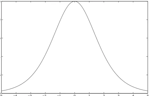
Let us have a closer look at (1.17). If W is invertible, the variance can be written as k∗ −k(x∗)t(W−1 +K)−1k(x∗) which has the same form as in the regression case, with W−1 replacing the noise covariance E. The following applies to the Bernoulli noise model introduced above. We have
wi = d2(−logσ(tiyi))/dy2i = σ(yi)(1−σ(yi)). Figure 1.1 shows wi plotted
against yi. How can we interpret that? Suppose that after we have found
ˆ
y we observe that most of the components in ˆy are close to 0, i.e. most of the training patterns actually lie in the critical region between the classes. Then, the elements in the “noise” matrix W−1 will be fairly small and the predictive variance will be rather small. On the other hand, if most of the components in ˆy are rather large, i.e. most of the patterns either deep in the region of their class or judged as strong outliers by the discriminant, W−1 has large elements, and the predictive variance will be large, for many cases x∗ close to the prior variance k∗. This is intuitively clear since patterns close to the decision boundary contain much more discriminative information (see discussion about Support Vectors below) than patterns far from the bound-ary, and a prediction based on more informative data should also be more confident than one based on a less informative sample.
−5 −4 −3 −2 −1 0 1 2 3 4 5 0 0.05 0.1 0.15 0.2 0.25 t y w
Figure 1.1: Component of W matrix againstty for the corresponding data-point.
An approximation to the predictive distribution for the class labelP(t∗|t) can be computed by averaging the noise distribution P(t∗|y∗) over the Gaussian
Pa(y∗|t). The analytically intractable integral can easily be approximated by
numerical techniques like Gaussian quadrature (see [PTVF92]). If the noise distributionP(t|y) is strictly monotonic increasing inty, there exist a unique threshold point a such that P(+1|y = a) = P(−1|y = a), and the optimal discriminant based on Pa(y∗|t) is g(x∗) = sgn(k(x∗)tK−1yˆ−a). In case of Bernoulli noise, we have a= 0.
The mode ˆy can be found very efficiently using the Newton-Raphson algo-rithm, which is equivalent to the Fisher scoring method mentioned above since we use the canonical link (recall subsection 1.2.6). Note that if the negative logarithm of the noise distribution P(t|y) is convex in y for both
t=±1, then the optimization problem of finding the mode is a convex one. Finally, we have to deal with the hyperparameters θ. The exact method would be to compute the posterior P(θ|D) and to average all quantities obtained so far by this distribution. Neither of these computations are tractable, so again approximations must be employed. Sophisticated Markov Chain Monte Carlo methods like the hybrid MC algorithm (see [Nea96]) can be used to approximate the integrals (see [WB98]). We can also search for the mode ˆθ of the posterior P(θ|D) and plug this parameter in, i.e.
P(y∗|D) ≈ P(y∗|D,θ), etc. Thisˆ maximum a-posteriori (MAP) approach can be justified in the limit of large datasets, since P(θ|D) converges to a delta or point distribution for all reasonable models. We will discuss the MAP approach in more detail below.
1.4
Support Vector classification
We follow [Vap98], [Bur98b]. If not otherwise stated, all facts mentioned here can be found in these references. Vapnik [Vap98] gives a fascinating overview of the history of Statistical Learning Theory and SVM.
Support Vector classification has its origin in a perceptron learning algorithm developed by Vapnik and Chervonenkis. They argued, using bounds derived within the newly created field of Statistical Learning Theory, that choosing the hyperplane which seperates a (linearly seperable) sample with maximum minimal margin6 results in a discriminant with low generalization error. The
minimal margin of a seperating hyperplaney(x) = (ω,x) +b, kωk= 1 with
6
In earlier literature, the minimal margin is sometimes simply referred to as margin. However, the margin (as defined in more recent papers) is actually a random variable whose distribution seems to be closely related to generalization error. The minimal margin is the sample minimum of this variable.
respect to the sample D is defined as min
i=1,...,ntiy(xi) (1.18)
where y(·) seperates the data without error. We will write yi = y(xi) in
the sequel. Note thattiyi denotes the perpendicular distance of xi from the
seperating plane. The reasoning behind this is that if the data points xi are
restricted to lie within a ball of radiusD/2, then the VC dimension of the set of hyperplanes with minimal margin M is bounded above by dD2/M2e+ 1
(see [Vap98]). Much later, theoptimum margin hyperplanes were generalized in two directions with the result being the Support Vector machine. First of all, nonlinear decision boundaries can be achieved by mapping the in-put vector x via Φ into a high, possibly infinite dimensional feature space with an inner product. Since in the original algorithm, input vectors oc-cured only in inner products, the nonlinear version is simply obtained by replacing such x by Φ(x) and inner products in X by inner products in the feature space. This seems to be a bad idea since neither Φ nor feature space inner products can usually be computed efficiently, but a certain rich class of Φ mappings have associated positive semidefinite kernels K such that K(x,x0) = (Φ(x),Φ(x0)). As we will see below, every positive semidefi-nite kernel satisfying certain regularity conditions actually induces a feature space and a mapping Φ. We will now derive the SVC algorithm using this nonlinear generalization, and later show how it arises as the special case of a more general setting.
Instead of constrainingω to unit length, we can equivalently fix the minimal margin to 1 (it must be positive if the data set is linearly seperable). Given a canonical hyperplane (ω, b), i.e.
tiyi ≥1, i= 1, . . . , n (1.19)
with equality for at least one point from each class, the same hyperplane with normal vector constrained to unit length has margin 1/kωk. The SVC problem therefore is to find a canonical hyperplane with minimal (1/2)kωk2. The second generalization was to allow for errors, i.e. violations of (1.19), but penalize errors [1−tiyi]+ using a monotonically increasing function of these
which is added to the criterion function. The fully generalized SVC problem is to find a discriminant y(x) = (ω,Φ(x)) +bwhich minimizes the functional
CX i [1−tiyi]++ 1 2kωk 2. (1.20)
This is a quadratic programming problem as can be shown by introducing nonnegative slack variables ξi, relaxing (1.19) to
tiyi≥1−ξi, i= 1, . . . , n (1.21)
and minimizing (1/2)kωk2 +CP
iξi with respect to (1.21). Note that the
sum is an upper bound on the number of training errors. Applying standard optimization techniques (see [Fle80]), we introduce nonnegative Lagrange multipliers αi ≥ 0 to account for the constraints (1.21) and νi ≥ 0 for the
nonnegativity of the slack variables. The multipliers are referred to as dual variables, as opposed to the primal variables ω and b. The Lagrangian has a saddlepoint7 at the solution of the original problem. Differentiating the
Lagrangian with respect to the primal variables and equating to zero, we can express ω in terms of the dual variables:
ω =
n
X
i=1
αitiΦ(xi). (1.22)
The primal variable b gives us the equality constraint
n
X
i=1
αiti = 0. (1.23)
Substituting these into the Lagrangian, we arrive at the Wolfe dual which depends only on the dual variables α:
X i αi− 1 2 X i,j αiαjtitj(Φ(xi),Φ(xj)). (1.24)
However, the combination of feasibility conditions8 andKarush-Kuhn-Tucker
(KKT) conditions introduces new constraints αi ≤C on the dual variables.
<