TSE‐607
“Beyond Truth‐Telling: Preference Estimation with
Centralized School Choice”
Gabrielle Fack, Julien Grenet and Yinghua He
Beyond Truth-Telling: Preference Estimation with
Centralized School Choice
Gabrielle Fack
Julien Grenet
Yinghua He
October 2015
Abstract
We propose novel approaches and tests for estimating student preferences with data from school choice mechanisms, e.g., the Gale-Shapley Deferred Acceptance. With-out requiring truth-telling to be the unique equilibrium, we show that the match-ing is (asymptotically) stable, or justified-envy-free, implymatch-ing that every student is assigned to her favorite school among those she is qualified for ex post. Having validated the methods in simulations, we apply them to data from Paris and reject truth-telling but not stability. Our estimates are then used to compare the sorting and welfare effects of alternative admission criteria prescribing how schools rank students in centralized mechanisms.
JEL Codes: C78, D47, D50, D61, I21
Keywords: Gale-Shapley Deferred Acceptance Mechanism, School Choice, Stable
Matching, Student Preferences, Admission Criteria
Fack: Universit´e Paris 1 Panth´eon-Sorbonne and Paris School of Economics, CES-Centre
d’ ´Economie de la Sorbonne, Maison des Sciences ´Economiques, 106-112 boulevard de l’Hˆopital, 75013 Paris, France (e-mail: [email protected]); Grenet: CNRS and Paris School of Eco-nomics, 48 boulevard Jourdan, 75014 Paris, France (e-mail: [email protected]); He: Toulouse School of Economics, Manufacture des Tabacs, 21 all´ee de Brienne, 31015 Toulouse, France (e-mail: [email protected]). For constructive comments, we thank Nikhil Agarwal, Peter Arcidiacono, Ed-uardo Azevedo, Estelle Cantillon, Yeon-Koo Che, Jeremy Fox, Guillaume Haeringer, Yu-Wei Hsieh, Adam Kapor, Fuhito Kojima, Jacob Leshno, Thierry Magnac, Ariel Pakes, Mar Reguant, Al Roth, Bernard Salani´e, Orie Shelef, Xiaoxia Shi, Matt Shum, and seminar/conference participants at Cal-tech, CES-ENS Cachan/RITM-UPSud, Columbia, Cowles Summer Conferences at Yale, EEA 2015 in Mannheim, ESWC 2015 in Montr´eal, IAAE 2014 in London, Matching in Practice 2014 in Berlin, Monash, Stanford, and Tilburg. The authors are grateful to the staff at the French Ministry of Education (Min-ist`ere de l’ ´Education Nationale, Direction de l’ ´Evaluation, de la Prospective et de la Performance) and those at the Paris Education Authority (Rectorat de l’Acad´emie de Paris) for their invaluable assistance in collecting the data. Financial support from the French National Research Agency (l’Agence Nationale de la Recherche) through Projects DesignEdu (ANR-14-CE30-0004) and FDA (ANR-14-FRAL-0005), from the European Union’s Seventh Framework Programme (FP7/2007–2013) under the Grant agree-ment no. 295298 (DYSMOIA), and from the Labex OSE is gratefully acknowledged.
Centralized mechanisms are common in the placement of students to public schools. Over the past decade, the Gale-Shapley Deferred Acceptance (DA) algorithm has become the leading mechanism for school choice reforms and has been adopted by many school districts around the world, including Amsterdam, Boston, New York, and Paris.
One of the reasons for the growing popularity of DA is the strategy-proofness of the mechanism (Abdulkadiro˘glu and S¨onmez, 2003). When applying for admission, students are asked to submit rank-order lists (ROLs) of schools, and it is in their best interest to rank schools truthfully. The mechanism therefore releases students and their parents from strategic considerations. As a consequence, it provides school districts “with more credible data about school choices, or parent ‘demand’ for particular schools,” as argued by the former Boston Public Schools superintendent Thomas Payzant when recommending DA in 2005. Indeed, such rank-ordered school choice data contain rich information on preferences over schools, and have been used extensively in the empirical literature, e.g., Ajayi (2013), Akyol and Krishna (2014), Burgess et al. (2014), Pathak and Shi (2014), and Abdulkadiro˘glu, Agarwal and Pathak (2015), among many others.
Due to the strategy-proofness of DA, one may be tempted to assume that the sub-mitted ROLs of schools reveal students’ true preferences. Strategy-proofness, however, means that truth-telling is only a weakly dominant strategy, which raises the potential issue of multiple equilibria because some students might achieve the same payoff by opt-ing for non-truth-tellopt-ing strategies in a given equilibrium. Makopt-ing truth-tellopt-ing even less likely, many applications of DA restrict the length of submittable ROLs, which destroys strategy-proofness (Haeringer and Klijn, 2009; Calsamiglia, Haeringer and Klijn, 2010).
The first contribution of our paper is to show how to estimate student preferences from school choice data under DA without assuming truth-telling. We derive identifying conditions based on a theoretical framework in which schools strictly rank applicants by some priority indices.1 Deviating from the literature, we introduce an application
cost that students have to pay when submitting ROLs, and the model therefore has the common real-life applications of DA as special cases. Assuming that both preferences
1School/university admission based on priority indices, e.g., academic grades, is common in many countries (e.g., Australia, China, France, Korea, Romania, Taiwan, and Turkey) as well as in the U.S. (e.g., “selective,” “exam,” or “magnet” schools in Boston, Chicago, and NYC). The website, www.matching-in-practice.eu, summarizes many other examples under the section “Matching Practices
and priorities are private information, we show that truth-telling in equilibrium is rather unlikely. For example, students would often omit a popular school if they expect a low chance of being accepted.
As an alternative, we consider a weaker assumption implied by truth-telling: stability, or justified-envy-freeness, of the matching outcome (Abdulkadiro˘glu and S¨onmez, 2003), which means that every student is assigned to her favorite school among all feasible ones. A school is feasible for a student if its ex post cutoff is lower than the student’s priority index. These cutoffs are well-defined and often observable: given an outcome, each school’s cutoff is the lowest priority index of the students accepted there. Conditional on the cutoffs, stability therefore defines a discrete model with personalized choice sets.
We show that stability is a plausible assumption: any equilibrium outcome of the game is asymptotically stable under certain conditions. When school capacities and the number of students are increased proportionally while the number of schools is fixed, the fraction of students not assigned to their favorite feasible school tends to zero in probability. Although stability, as an ex post optimality condition, is not guaranteed in such an incomplete-information game if the market size is arbitrary, we provide evidence suggesting that typical real-life markets are sufficiently large for this assumption to hold. Based on the theoretical results, we propose a menu of approaches for preference estimation. Both truth-telling and stability lead to maximum likelihood estimation under the usual parametric assumptions. We also provide a solution if neither assumption is satisfied: as long as students do not play dominated strategies, the submitted ROLs reveal true partial preference orders of schools (Haeringer and Klijn, 2009),2 which allows us to
derive probability bounds for one school being preferred to another. The corresponding moment inequalities can be used for inference using the related methods (for a survey, see Tamer, 2010). When stability is satisfied, these inequalities provide over-identifying information that can improve estimation efficiency (Moon and Schorfheide, 2009).
To guide the choice between these identifying assumptions, we consider several tests. Truth-telling—consistent and efficient under the null hypothesis—can be tested against stability—consistent but inefficient under the null—using the Hausman test (Hausman, 1978). Moreover, stability can be tested against undominated strategies: if the outcome is unstable, the stability conditions are incompatible with the moment inequalities implied
by undominated strategies, allowing us to use tests such as Bugni, Canay and Shi (2014). Applying the methods to school choice data from Paris, our paper makes a second contribution by empirically studying the design of the admission criteria that determine how schools rank students. Despite the fact that admission criteria impact student sorting and student welfare by prescribing which students choose first, they have been relatively under-studied in the literature (see the survey by Pathak, 2011).3 Our empirical
evalua-tion of the commonly-used criteria thus provides new insights into the design of student assignment systems.
The data contain 1,590 middle school students competing for admission to 11 academic-track high schools in the Southern District of Paris. As dictated by the admission cri-terion, schools rank students by their academic grades but give priority to low-income students. The emphasis on grades induces a high degree of stratification in the average peer quality of schools, which is essential for identifying student preferences.
To consistently estimate the preferences of the Parisian students, we apply our pro-posed approaches and tests, after validating them in Monte Carlo simulations. Truth-telling is strongly rejected in the data, but not stability. Incorrectly imposing truth-Truth-telling leads to a serious under-estimation of preferences for popular or small schools.
We use our preferred estimates to perform counterfactual analyses of the admission criteria. By assuming that students form preferences based on the characteristics of those who are already attending the school, our static model incorporates “dynamics”. We therefore simulate equilibrium outcomes under each admission criterion in both the short run and the long run. Holding constant how student preferences are determined, the short-run outcomes measure what happens in the first year after we replace the current criterion with an alternative; the long-run outcomes are to be observed in steady state.
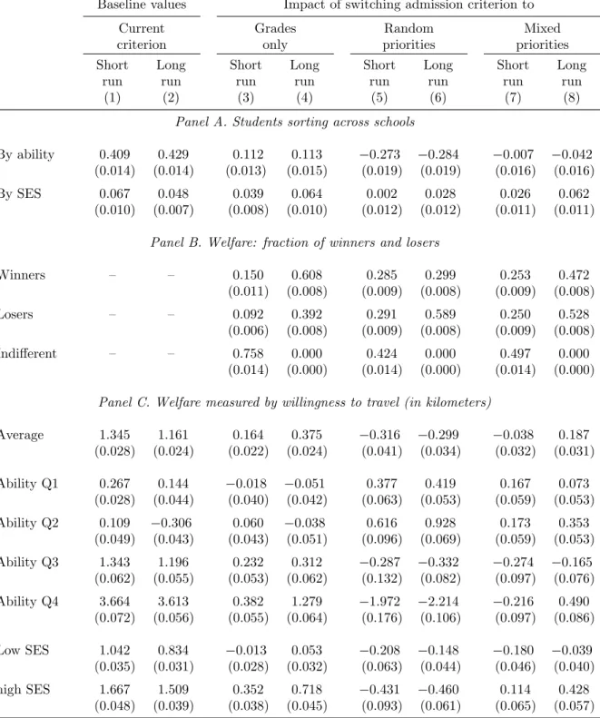
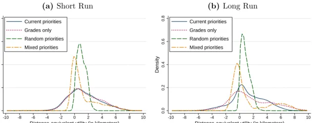
The admission criteria that we consider differ in their weighting of two factors: aca-demic grades and random priorities from lotteries. The results show that random pri-orities would substantially lower sorting by ability, compared with the current policy, but would slightly raise sorting by socioeconomic status (SES). By contrast, a grades-only policy would substantially increase sorting by SES. This is largely because of the low-income priority in the current admission criterion. We also consider mixed priorities
where the “top two” schools select students based on grades, while admission to other schools is based on random priorities. This policy would lower sorting by ability but increase sorting by SES. In general, results are more pronounced in the long run, because school attributes evolve over time. The welfare analysis highlights the trade-off between the welfare of low- and high-ability students, in both the short run and the long run, under the grades-only or random-priorities policies. However, under the mixed-priorities criterion, this trade-off is mitigated in the long run. Overall, mixed priorities appear as a promising candidate to enhance overall welfare with modest effects on sorting, while balancing the welfare of low- and high-ability students.
Other Related Literature. Our results on asymptotic stability in Bayesian Nash equilibrium are in line with Haeringer and Klijn (2009), Romero-Medina (1998) and Ergin and S¨onmez (2006), who prove the stability of Nash equilibrium outcomes under the constrained DA or the Boston mechanism. Although stability is a rather common identifying assumption in the two-sided matching literature (see the surveys by Fox, 2009; Chiappori and Salani´e, forthcoming), it has not, to our knowledge, been used in empirical studies of school choice except in Akyol and Krishna (2014). Observing the matching outcome and the cutoffs of high school admissions in Turkey, the authors estimate preferences based on the assumption that every student is assigned to her favorite feasible school. This assumption is formalized and justified in our paper. Moreover, beyond stability, we propose approaches that incorporate the information from ROLs and that fully endogenize the cutoffs.
Large markets are commonly considered in theoretical studies on the properties of mechanisms (see the survey by Kojima, 2015). Closely related is Azevedo and Leshno (forthcoming), who show the asymptotics of the cutoffs of stable matchings. Our paper extends their results to Bayesian Nash equilibrium.
There is also a growing literature on preference estimation under other school choice mechanisms, e.g., the Boston mechanism (Agarwal and Somaini, 2014; Calsamiglia, Fu and G¨uell, 2014; He, 2015). Since this mechanism is not strategy-proof (Abdulkadiro˘glu and S¨onmez, 2003), observed ROLs are sometimes considered as maximizing expected utility. Taking estimated admission probabilities as students’ beliefs, one could apply the same approach to our setting, i.e., a discrete choice problem defined on the set of possible ROLs. Agarwal and Somaini (2014) show how preferences can be non-parametrically
identified when admission probabilities are non-degenerate.4
Organization of the Paper. The paper proceeds as follows. Section 1 presents the model that provides our theoretical foundation for preference estimation. Section 2 discusses the corresponding empirical approaches and tests, which are illustrated in Monte Carlo simulations. School choice in Paris, and our results on estimation and testing with the Parisian data, are shown in Section 3. The counterfactual analyses of commonly-observed admission criteria are described in Section 4. Section 5 concludes.
1
The Model
A (finite) school choice problem is denoted by F
!
rui,s, ei,ssiPI,sPS,tqsusPS, Cp||q )
, where I t1, . . . , Iu is the set of students, and S t1, . . . , Su is the set of schools. Studentihas a von Neumann-Morgenstern (vNM) utilityui,s P r0,1sof being assigned to
s, and, as required by the admission criterion, school s ranks students by priority indices
ei,s P r0,1s, i.e., s “prefers” i over j if and only if ei,s ¡ ej,s. To simplify notation, we
assume that there are no indifferences in either vNM utilities or priority indices, and that all schools and students are acceptable. Each school has a positive capacity qs.
Schools first announce their capacities, and every student then submits a rank-order list (ROL) of Ki ¤ S schools, denoted by Li l1i, . . . , l
Ki
i
, where lk
i P S is i’s kth
choice. Li also represents the set of schools being ranked in Li. We define ¡Li such
that s ¡Li s1 if and only if s is ranked above s1 inLi. The set of all possible ROLs is L,
which includes all ROLs ranking at least one school. Studenti’s true ordinal preference is
Ri ri1, . . . , riS
PL, which ranks all schools according to cardinal preferences rui,sssPS.
When submitting a ROL, a student incurs a costCp|L|q, which depends on the number of schools being ranked in L, |L|. Furthermore, Cp|L|q P r0, 8s for all L and is weakly increasing in |L|. To simplify students’ participation decision, we set Cp1q 0.
Such a cost function flexibly captures many common applications of school choice mechanisms. IfCp|L|q 0 for allL, we are in the traditional setting without costs (e.g., Abdulkadiro˘glu and S¨onmez, 2003); if Cp|L|q 8 for |L| greater than a constant K, it corresponds to the constrained school choice where one cannot rank more thanK schools (e.g., Haeringer and Klijn, 2009); whenCp|L|q cp|L| Kq, one has to pay a unit costc
for each choice beyond the firstK choices (e.g., Bir´o, 2012); the monotonic cost function can simply reflect that it is cognitively burdensome to rank too many choices.
The student-school match is solved by a mechanism that takes into account students’ ROLs and schools’ rankings over students. Our main analysis focuses on the student-proposing Gale-Shapley Deferred Acceptance (DA), leaving the discussion of other mech-anisms to Section 1.5. DA, as a computerized algorithm, works as follows:
Round 1. Every student applies to her first choice. Each school rejects the lowest-ranked students in excess of its capacity and temporarily holds the other students.
Generally, in:
Round k. Every student who is rejected in Round pk1q applies to the next choice on her list. Each school, pooling together new applicants and those who are held from Round pk1q, rejects the lowest-ranked students in excess of its capacity. Those who are not rejected are temporarily held by the schools.
The process terminates after any Round k when no rejections are issued. Each school is then matched with the students it is currently holding.
We introduce the following definition of many-to-one matching.
Definition 1. A matching µ is a function from the set IYS into the set of unordered families of elements ofIYS such that: (i)|µpiq | 1 for every studenti; (ii) |µpsq | qs
for every school, and if the number of students in µpsq, say ns, is less than qs, thenµpsq
contains qsns copies of s itself; and (iii) µpiq s if and only if iP µpsq.
1.1
Information Structure and Decision-Making
We assume that every student’s preferences and indices are private information, and are i.i.d. draws from a joint distribution Gpv|eq Hpeq, which is common knowledge.5
Given others’ indices and submitted ROLs (Li,ei),i’s probability of being assigned
tos is a function of her priority index vectorei and submitted ROL Li:
aspLi, ei;Li, eiq $ & % Pr i is rejected by l1 i, . . . , lki and accepted byl k 1 i s|Li, ei;Li, ei 0 if s PLi if s RLi
5The analysis can be extended to allow priority indices to be common knowledge, after conditioning on a realization ofrei,ssiPI,sPS.
Clearly, given the algorithm, aspLi, ei;Li, eiqis either zero or one for all s.
Student i’s strategy is σpvi, eiq : r0,1sS r0,1sS Ñ∆pLq. We consider a symmetric
equilibriumσ such thatσsolves the following maximization problem for every student:6
σpui, eiq Parg max σ # ¸ sPS ui,s » » aspσ, ei;σpui, eiq, eiqdGpui|eiqdHpeiq Cp|σ|q + ,
whenσpui, eiqis a pure strategy.7 The existence of pure-strategy Bayesian Nash
equilib-rium can be established by applying Theorem 4 (Purification Theorem) in Milgrom and Weber (1985), although there might be multiple equilibria.
Given an equilibriumσand a realization of the economyF, we observe one matching,
µpF,σq, such that theex post cutoff (or shadow price) of each school is:
ps µpF,σq $ & % min ei,s|iPµpF,σqpsq ( 0 if sR µpF,σqpsq if sP µpF,σqpsq That is, ps µpF,σq
is zero if s does not meet its capacity; otherwise, it is the lowest index among all accepted students. The vector of cutoffs is denoted by PpµpF,σqq. In
what follows, we sometimes shorten ps µpF,σq
to ps when there is no confusion. With
the cutoff, we can redefine the admission probabilities as:
aspLi, ei;Li, eiq
$ & %
Pr ps1 ¡ei,s1 for s1 l1i, . . . , lki and ps ¤ei,s for slik 1 |L, Li, ei
0
if s PLi
if s RLi
1.2
Truth-Telling Behavior in Equilibrium
To assess how plausible the truth-telling assumption is in empirical studies, we begin by investigating students’ truth-telling behavior in equilibrium.
Definition 2. Student i is weakly truth-telling if her ROL Li ranks truthfully her
top |Li| choices, i.e., ui,lk
i ¡ ui,lki 1 for all l
k i, l
k 1
i P Li, and ui,s ¡ ui,s1 for all s P Li
and s1 R Li. If a weakly truth-telling Li is a full list and thus Li Ri, i is strictly
truth-telling.
It is well known that DA is strategy-proof when there is no application cost.
Theorem 1 (Dubins and Freedman, 1981; Roth, 1982). When Cp|L|q 0 for all L P L, the student-proposing DA is strategy-proof: strict truth-telling is a weakly dominant strategy for all students.
The above theorem, however, highlights the possibility of multiple equilibria: there might exist strategies that are payoff-equivalent to truth-telling in some equilibrium. If we assume that the equilibrium where everyone is truth-telling is always selected, we implicitly impose a selection rule that may not be reasonable in real life. It is therefore useful to clarify the conditions under which strict truth-telling is a strictly dominant strategy and thus the unique equilibrium, for which we need the following definition.
Definition 3. Fix any iand two ROLs, Li andL1i, such that the only difference between
them is two neighboring choices: plik, lik 1q ps, s1q,pli1k, l1ik 1q ps1, sq, and lki li1k
for all k k, k 1. A mechanism satisfies swap monotonicity if for all pLi, eiq:
aspLi, ei;Li, eiq ¥aspL1i, ei;Li, eiq;as1pLi, ei;Li, eiq ¤ as1pL1i, ei;Li, eiq.
These two conditions are either both strict or both equalities. If they are strict for any pair of ps, s1q given any pLi, ei;Li, eiq, the mechanism is strictly swap monotonic.
DA is swap monotonic, but not strictly swap monotonic (Mennle and Seuken, 2014).8
Theorem 2. Strict truth-telling is a strictly dominant strategy under DA if and only if (i) there is no application cost: Cp|L|q 0, @LP L; and
(ii) the mechanism is strictly swap monotonic.
All proofs can be found in Appendix A. The first condition is violated if students cannot rank as many schools as they wish, or if they suffer a cognitive burden when ranking too many schools. More importantly, DA does not satisfy the second condition. Taking one step back, one might be interested in a (Bayesian) Nash equilibrium where truth-telling is a strict, and thus unique, best response given that others are truth-telling.
Proposition 1. When others are truth-telling,σi Ri, it is a strict best response for
i to report true preferences, σi Ri, if and only if:
8Strict swap monotonicity requires that, given any ROLs of others, i’s admission probability at s strictly increases whenever s is moved up one position in i’s ROL. It is certainly violated under DA when, for example, everyone else ranks onlysin their ROLs.
(i) there is no application cost: Cp|L|q 0, @LP L; and
(ii) the mechanism is strictly swap monotonic given σi Ri.
Again, the second condition, although being relaxed, is still restrictive, as one may not want to restrict Ri in empirical studies.9
We call Li, |Li| ¤S, a true partial preference order of schools if Li respects the
true preference ordering among those ranked in Li. That is, ifs is ranked befores1 inLi,
then s is also ranked before s1 according to i’s true preference Ri; when s is not ranked
inLi, its is not possible to determine how s is ranked relative to any other school.
Theorem 3. Under DA with cost Cp|L|q, it is a weakly dominated strategy to submit a ROL that is not a true partial preference order. If the mechanism is strictly swap monotonic, such strategies are strictly dominated.
Theorem 3 implies that under the truncated DA, untrue partial order is a dominated strategy (Haeringer and Klijn, 2009).
1.3
Matching Outcome: Stability
The above results show that the truth-telling assumption is rather restrictive in empirical studies. We now turn instead to the properties of equilibrium matching outcomes.
Definition 4. Given a matching µ, pi, sq form a blocking pair if (i) i prefers s over her matched school µpiq while s has an empty seat (s P µpsq), or if (ii) i prefers s over
µpiq while s has no empty seats (sRµpsq) but i’s priority index is higher than its cutoff,
ei,s ¡mintjPµpsqupej,sq. µis stable if there is no blocking pair.
Stability is a concept borrowed from two-sided matching and is also known as elimi-nation of justified envy in school choice (Abdulkadiro˘glu and S¨onmez, 2003). In our setting, stability can be conveniently linked to schools’ cutoffs. Given a matching µ, school s isfeasible fori if pspµq ¤ei,s, and we denote the set of feasible schools for iby
Spei, Ppµqq. We then have the following lemma, whose straightforward proof is omitted.
Lemma 1. µ is stable if and only if µpiq arg maxsPSpei,Ppµqqui,s for all i P I; i.e., all
students are assigned to their favorite feasible school.
It is well known that DA always produces a stable matching when students are strictly truth-telling (Gale and Shapley, 1962), but not when they are only weakly truth-telling. We have, however, the following result linking weak truth-telling and stability.
Proposition 2. Suppose everyone is weakly truth-telling under DA. Given a matching: (i) every assigned student is assigned to her favorite feasible school; and
(ii) if everyone is assigned to a school, the matching is stable.
We are also interested in implementing stable matchings in dominant strategies, which would free us from specifying the information structure and from imposing additional equilibrium conditions. The following theorem provides the necessary and sufficient con-ditions for such dominant-strategy implementations, which are again rather restrictive.
Proposition 3. Under DA, stable matching can be implemented in dominant strategies if and only ifCp|L|q 0for allL. If additionally the mechanism is strictly swap monotonic, stable matching can be implemented in strictly dominant strategies.
1.4
Asymptotic Stability in Bayesian Nash Equilibrium
So far, we have shown that neither truth-telling nor stability is satisfied without a set of restrictive assumptions. Following the literature on large markets, we study whether stability of the equilibrium outcome can be asymptotically satisfied.
1.4.1 Randomly Generated Finite Economies and the Continuum Economy
We consider a sequence of randomly generated finite economiestFpIqu
IPN, such that FpIq ! rui,s, ei,ssiPIpIq,sPS, qp Iq s ( sPS, Cp|L|q ) ;
(i) There are I students inFpIq, whose types are i.i.d. draws from GH;
(ii) Each school’s capacity relative to I remains constant, i.e., qspIq{I q¯s for all s,
where ¯qs is a positive constant.10
Each finite economy naturally leads to an empirical (joint) distribution of types, which converges to GH.11 We further define a continuum economyE, where:
10To simplify notation, we ignore the fact that capacities in finite economies are integers.
11Here the convergence notion is the weak convergence of measures, which is defined as³XdGˆpIqHˆpIqÑ
³
XdGdH for every bounded continuous functionX :r0,1sS r0,1sS ÑR. This is also known as narrow convergence or weak-* convergence.
(i) A mass one of students, I, have types in space r0,1sS r0,1sS associated with a (probability) measure GH;
(ii) School s has a positive capacity ¯qs.
The definitions of DA and stability can be naturally extended to continuum economies as in Azevedo and Leshno (forthcoming), who also establish the existence of stable match-ing in such settmatch-ings. In a stable matchmatch-ing ofE, the demand for schools is the measure of students whose priority index is above s’s cutoff and whose favorite feasible school is s:
DspPq
» »
1psarg max
s1PSpei,Pq
tus1uqdGpu|eqdHpeq,
which is differentiable with respect to rpsssPS in usual applications (see Appendix A.4).
1.4.2 Results
We first present results on stable matchings in both finite and continuum economies, and then discuss whether stable matching can be achieved in equilibrium.
It is known that generically, there exists a unique stable matching in the contin-uum economy (Azevedo and Leshno, forthcoming), and we denote this matching in E
as µ8. Although µ8 is unique, there could exist some Nash equilibrium that leads to an unstable matching. We discuss this in Appendix A.4, and results are summarized in Proposition A1. In the following, we assume that all Nash equilibria of the contin-uum economy E result in the stable matching, which in practice can be checked using Proposition A1.
Linking finite and continuum economies, the next result shows that, as the market size grows, the only strategies that can survive in finite economies are those ranking µ8.
Proposition 4. If a strategy σ: r0,1sS r0,1sS Ñ ∆pLq results in a matching in the
continuum economy µpE,σq such that GHpti P I | µpE,σqpiq µ8piquq ¡ 0 in E, then
there must exist N such that σ is not an equilibrium in FpIq for all I ¡N.
When Cp2q ¡0, we can obtain even sharper results:
Lemma 2. If Cp2q ¡ 0 and σpui, eiq µ8piq for all i almost surely, then there exists N
enough, such Bayesian Nash equilibria are the only possible equilibria. It also implies that everyi includes µ8piq almost surely inσpIq.12
Given the finite economies, when σpJq is in pure strategy, it creates a sequence of
ordinal economies, FσpIpJqq ! rσpJqpu i, eiq, eisiPIpIq,rqp Iq s ssPS, Cp|L|q )
. The original cardinal preferences rui,ssiPIpIq,sPS are replaced by ordinal “preferences” rσpJqpui, eiqsiPIpIq.
Corre-spondingly, the continuum ordinal economy isEσpJq such thatFp
Iq
σpJq ÑEσpJq almost surely.
If σpJq is in mixed strategies, a distribution of economies can be similarly constructed. GivenEσpJq, assuming that everyone reports true ordinal preferences leads to a
match-ing that is stable with respect to rσpJqpui, eiqsiPI. In this matching, the demand for each
school in EσpJq as a function of the cutoffs is:
DspP, σpJqq » » 1pus max s1PSpei,PqσpJqpui,eiq tus1uqdGpui |eiqdHpeiq, whereσpJqpu
i, eiqalso denotes the set of schools ranked byi. LetDpP, σpJqq rDspP, σpJqqssPS.
Proposition 5. Fix σpJqP tσpIquIPN, where σpJq is a Bayesian Nash equilibrium of FpIq, and apply it to the sequence of finite economies tFpIqu
IPN. We then have: (i) supJPN||PpµpFpIq,σpJqqq P8||ÑÝp 0, and, therefore, PpµpFpJq,σpJqqqÝÑp P8.
(ii) F ractionpstudents in any blocking pair in µpFpJq,σpJqqqÝÑp 0.
(iii) If EσpJq has a C1 demand function and BDpP8, σpJqq{BP8 is nonsingular, the
asymptotic distribution of cutoffs in FpIq is:
?
I PpµpFpIq,σpJqqq P8
d
Ý
ÑNp0, VpσpJqqq
where P8 is the cutoff vector in E, VpσpJqq BDpP8, σpJqq1Σ BDpP8, σpJqq11, and
Σ q1p1q1q q1q2 q1qS q2q1 q2p1q2q ... .. . ... . .. qS1qS qSq1 qSqS1 qSp1qSq .
Proposition 5 shows that the matching is asymptotically stable. It also sheds light on the convergence rate.
1.4.3 Comparative Statics: Probability of Observing a Blocking Pair
Based on the above results, we can discuss “comparative statics” to evaluate how market size, the cost of submitting a list, and other factors affect the probability of observing an
ex post blocking pair in equilibrium.
Let us consider a finite economy FpIq where the Bayesian Nash equilibrium being
played is σpIq. Without loss of generality, it is a pure strategy, i.e., σpIqpui, eiq Li.
Proposition 6. In a Bayesian Nash equilibrium outcome, where Li represents a true
partial order of i’s ordinal preferences, ex post i can form a blocking pair only with a school that is not ranked in Li. The probability that i is in a blocking pair:
(i) is bounded above by a term that is increasing in the cost of including an additional school, Cp|Li| 1q Cp|Li|q, and decreasing in the cardinal utilities of omitted
schools relative to the less preferable ones in Li; and
(ii) decreases to zero as market size, I, goes to infinity.
Remark 1. Proposition 6 has implications for empirical studies. Stability is more plau-sibly satisfied when the cost of ranking more schools is lower, and/or the market is large. Moreover, in the case of constrained/truncated DA where there is a limit on the length of ROLs, the more schools are allowed to be ranked, the more likely stability is to be satisfied.
1.5
Discussion and Extensions
Non-Equilibrium Strategies. We have thus far focused on the case in which everyone plays an equilibrium strategy with a common prior, which is rather restrictive. More realistically, some students could have different information and make mistakes when strategizing.13
When introducing the empirical approaches, we take this possibility into account. If students do not play equilibrium strategies, the matching is less likely to be stable. Therefore, allowing students to play non-equilibrium strategies amounts to having un-stable matching outcomes. In Section 2.7, we propose a test for stability, which is then also a test for non-equilibrium strategies. If stability is rejected, one can obtain
identi-undominated strategies. Theorem 3 provides the theoretical foundation for the approach to be introduced in Section 2.6.
Uncertainty in Priority Indices. In reality, it is common that there is some ex ante
uncertainty in schools’ rankings over students. For example, students in some Chinese provinces do not know their exact test scores when applying to universities. In extreme cases, school choice in places such as Beijing and NYC uses an ex ante unknown lottery to rank students.
Our main analysis of finite economies allows a certain degree of uncertainty in priority indices, in that every student knows her own indices but not her precise ranking among all students; importantly, this uncertainty degenerates with market size. In the case of non-degenerate uncertainty, the fraction of students who can form at least one blocking pair with some school is small if the uncertainty is limited and the market size is large.14
Beyond School Choice. Although the analysis has focused on school choice, or col-lege admission, our results apply to other assignment/matching based on DA or similar centralized mechanisms. The key requirement is that researchers have information on the “preferences” of the agents on one side, i.e., how they rank the agents on the other side.15 Examples include teacher assignment to public schools in France and the Scottish
Foundation Allocation Scheme matching medical school graduates to training programs, which are both centralized.16 The estimation approaches discussed in Section 2 could be
implemented in these settings.
Other Mechanisms. Our main theoretical results can be applied to another two pop-ular mechanisms, the school-proposing DA and the Boston mechanism (see definition in Appendix E). In the school-proposing DA, schools propose to students following the order of student priority indices. When considering either of these mechanisms, Theorem 3 no longer holds; that is, students might have incentives not to report a true partial preference
14This is shown in Monte Carlo exercises, the results of which are available upon request. In the case where schools rank students by lotteries,ex post optimality (i.e., stability) is less likely to be satisfied in Bayesian Nash equilibrium. For estimation in school choice with such non-degenerate uncertainties, one can use the approaches in Agarwal and Somaini (2014), Calsamiglia et al. (2014), and He (2015).
15When researchers have no information on how either side ranks the other, we are in the classic setting of two-sided matching, where additional assumptions are often needed for identification and estimation. 16Details can be found on the website of the “Matching in Practice” network at www.matching-in-practice.eu/matching-practices-of-teachers-to-schools-france, and www.matching-in-practice.eu/the-scottish-foundation-allocation-scheme-sfas, respectively.
order (Abdulkadiro˘glu and S¨onmez, 2003; Haeringer and Klijn, 2009). Nonetheless, the asymptotic stability result (Proposition 5) still holds, as its proof does not rely on Theo-rem 3. Indeed, it is known that the matching outcome can be stable in Nash equilibrium for both mechanisms (Ergin and S¨onmez, 2006; Haeringer and Klijn, 2009). It should be noted that when schools rank students strictly, the Boston mechanism is approximated by the DA where everyone can rank only one school, which imposes an infinite cost on rank-ing more than one school; therefore, one would need a larger market to ensure stability (Proposition 6).
Obviously, (asymptotic) stability does not hold under unstable mechanisms such as the Top-Trading Cycles (Abdulkadiro˘glu and S¨onmez, 2003).
2
Empirical Approaches
Building on the theoretical results from the previous section, we explain how to estimate student preferences under different sets of assumptions and propose a series of tests to select the appropriate approach. To be more concrete, we consider a logit-type random utility model, although our approaches can be extended to other specifications.
2.1
Model Setting
Throughout this section, we consider a market in whichIstudents compete for admission intoS distinct schools. Each schoolshas a positive capacityqs, and students are assigned
through the student-proposing DA.
Student i’s utility from attending schools s is defined as:
ui,sσVi,s σi,s αsdi,s Z1i,sβ σi,s,
whereσVi,s αsdi,s Z1i,sβdenotes the deterministic component of utility andσi,s PR
denotes unobserved heterogeneity; σ is a scaling parameter; αs is school s’s fixed effect;
Zi,s PRKare student-school specific attributes, e.g., interactions of student characteristics
and school attributes; di,s is the distance from i’s home to school s. It is convenient to
estimated, (tαsusPS,β, σ). We normalize the utility functions by setting α1 0. Such a
formulation rules out outside options, although this assumption can be relaxed. Finally, we assume that i KZi, and that i,s is i.i.d. over i and s with the type-I extreme value
(Gumbel) distribution.
2.2
Truth-Telling
Despite its likely implausibility, we start with formalizing the estimation under the truth-telling assumption. If each studenti is weakly truth-telling and submitsKi |Li| (¤S)
choices, then Li pli1, . . . , l Ki
i q ranks truthfully i’s top Ki choices. The probability of
observing student isubmitting Li is:
Prpi submitsLi |Zi;θq
Pr Li pl1i, . . . , l Ki
i q |Zi;θ;Ki
Prpi submits a ROL of length Ki |Zi;θq.
We can follow the literature in assuming that Ki is orthogonal toui,s, for all s(Hastings,
Kane and Staiger, 2008; Abdulkadiro˘glu et al., 2015), which allows to ignore the first term and focus instead on the following conditional choice probability:17
Pr Li pl1i, . . . , l Ki i q |Zi;θ;Ki Pr ui,l1 i ¡ ¡ui,liKi ¡ui,s1 @s 1 P SzL i |Zi;θ;Ki ¹ sPLi exppVi,sq ° s1£LisexppVi,s1q
where s1 £Li s indicates that s1 is not ranked before s inLi, which includes s itself and
the schools not ranked in Li. This rank-ordered (or “exploded”) logit model can be seen
as a series of conditional logit models: one for the top-ranked school (li1) being the most preferred; another for the second-ranked school (l2
i) being preferred to all schools except
the one ranked first, and so on.
The model is point identified under the usual assumptions and can be estimated by maximum likelihood estimation (MLE) with the log-likelihood function:
lnLT T θ|Z,|L| I ¸ i1 ¸ sPLi Vi,s I ¸ i1 ¸ sPLi ln ¸ s1£Lis exppVi,s1q ,
17This assumption is justified when the length of a ROL is determined by institutional arrangements. Alternatively, one may consider that the length of ROLs depends on the number of schools that are preferred to the outside option, which could violate the above assumption.
where |L|is the length of all ROLs. The estimate is denoted by ˆθT T.
2.3
Stability
Stability of the matching outcome implies that every student is assigned to her favorite school among those she is qualified for ex post. We are interested in the probability of the observed matching µ being realized. Given µ, we also observe the vector of cutoffs,
Ppµq rpsssPS, which defines each student’s set of feasible schools, Spei, Pq. This set
includes every schoolswhose admission cutoffps is below the student’s index ei,sat that
school. The probability of observing µ conditional on the full matrix of observablespZq, and the parameters θ is then:
Pr
a stable matching µbeing realized|Z;θ
Pr
cutoffs arePpµq;µpiq arg max
s1PSpei,Pq pui,s1q,@iPI |Z;θ Pr cutoffs arePpµq |Z;θ ¹ iPI Pr µpiq arg max s1PSpei,Pq pui,s1q |Zi, Ppµq;θ .
The first equation reflects the fact that a stable matching can be fully characterized by the cutoffs Ppµq and by students being matched with their favorite school given Ppµq; the last equation is implied by the i.i.d. assumption on student preferences and by the assumption that the individual student’si has no impact onPpµq.
Note that the probability, Pr µpiq arg maxs1PSpei,Pqpui,s1q,@iP I |Z, Ppµq;θ
, ex-plicitly conditions on the cutoffs Ppµq, highlighting the fact that we use the cutoffs to specify each student’s set of feasible schools Spei, Pq. However, Ppµqdoes not affect the
probability beyond that, as preferences do not depend on cutoffs. Therefore, Pr µpiq arg max s1PSpei,Pq pui,s1q,@iP I |Z, Ppµq;θ Pr µpiq arg max s1PSpei,Pq pui,s1q,@iPI |Z;θ ¥Pr
a stable matching µis realized |Z;θ ,
where the last inequality becomes an equality only when there is a unique stable matching conditional on pZ,θq, i.e., Prpcutoffs arePpµq |Z;θq 1. The multiplicity of stable matchings and thus of cutoffs conditional onpZ,θqcomes from the randomness in utility shocks, , as well as from the potential multiplicity of stable matchings given.
tional) log-likelihood function is: lnLSTpθ|Z, µq I ¸ i1 Vi,µpiq I ¸ i1 ln ¸ s1PSi exppVi,s1q ln Pr cutoff is Ppµq |Z;θ . (1) The last term above deserves some careful discussion, because we do not have an analytic form of this probability. In a finite economy, the distribution of cutoffs is approximated by the asymptotic normal distribution derived in Proposition 5, which provides a solution:
ln
Pr cutoff is Ppµq |Z;θ lnφ
Ppµq P8pZ,θq, V pZ,θq {I ,
where φpqis the density function of the |S|-dimensional normal distribution; P8pZ,θq
is the vector of cutoffs for the unique stable matching in the continuum economy given
pZ,θq; and V pZ,θqis the asymptotic variance calculated based on the formula in Propo-sition 5. Both terms can be calculated by the simulation methods set out in Appendix C.18
With this approximation, the model can be estimated by MLE as well, and the estima-tor is denoted by ˆθST. Note that we can omit the term, Prpcutoff isPpµq |Z;θq, when
there is a unique stable matching, e.g., in large enough economies. In our applications, we report results both with and without the cutoff term in the likelihood function.
2.4
Testing Truth-Telling against Stability
Having two distinct estimates ˆθT T and ˆθST for the parameters of the school choice model
provides an opportunity to test the truth-telling assumption against the stability assump-tion by carrying out a Hausman-type specificaassump-tion test.
As summarized in Proposition 2, if every student is weakly truth-telling and is assigned to a school, the matching outcome is stable. Stability, however, does not imply that students are weakly truth-telling and is therefore a less restrictive assumption. Under the null hypothesis that students are weakly truth-telling, both estimators are consistent but only ˆθT T is asymptotically efficient. Under the alternative that the matching outcome
is stable but students are not weakly truth-telling, only ˆθST is consistent.
In this setting, the general specification test developed by Hausman (1978) can be
18 In the application, we approximate the joint probability density function at the true variances but zero pairwise correlations. This is justified, because these correlations are small. In the Monte Carlo samples discussed in Appendix C, the true covariance matrix shows that the average of all the off-diagonal terms is only 3.5 percent of the average of all the diagonal terms.
applied by computing the following test statistic:
TH pθˆST θˆT Tq1pVˆST VˆT Tq1pθˆST θˆT Tq,
where pVˆST VˆT Tq1 is the inverse of the difference between the asymptotic covariance
matrices of ˆθST and ˆθT T. Under the null hypothesis, TH χ2pdθq, where dθ is the
dimension ofθ. If the model is correctly specified and the matching is stable, the rejection of the null hypothesis implies that (weak) truth-telling is violated in the data.
2.5
Stability and Undominated Strategies
An important advantage of the stability assumption is that it only requires data on the assignment outcomes. However, as submitted ROLs are often observed, one might prefer to use the identifying information contained in such data as well.
Under the rationality assumption that students play undominated strategies, observed ROLs are students’ true partial preference orders in the context of the student-proposing DA. That is, every Li respects student i’s true preference ordering among the schools
ranked in Li. These partial orders provide over-identifying information that can be used
in combination with the stability assumption to estimate student preferences.
The potential benefits from this approach can be illustrated through a simple example. Consider a constrained/truncated DA where students are only allowed to rank up to three schools out of four. With personalized sets of feasible schools under the stability assumption, the preferences over two schools, says1ands2, are estimated mainly from the
sub-sample of students who are assigned to either of these schools while having priority indices above the cutoffs of both. Yet it is possible that all students include s1 and s2
in their ROLs, even if these schools are not ex post feasible for some students. In such a situation, all students could be used to estimate the preference ranking of s1 and s2,
rather than just a sub-sample. As shown below, this argument can be extended to the case where two or more schools are observed being ranked by a subset of students.
Moment inequalities. Students’ ROLs can be used to form over-identifying condi-tional moment inequalities. Without loss of generality, consider two schools s1 and s2.
Since not everyone ranks both schools, the probability of i rankings1 befores2 is:
Prps1 ¡Li s2|Zi;θq Prpui,s1 ¡ui,s2 and s1, s2 PLi|Zi;θq ¤Prpui,s1 ¡ui,s2|Zi;θq (2)
The first equality is because of undominated strategy, and the inequality defines a lower bound for the probability of ui,s1 ¡ui,s2. Similarly, one can derive an upper bound:
Prpui,s1 ¡ui,s2 |Zi;θq ¤1Prps2 ¡Li s1 |Zi;θq (3)
Inequalities (2) and (3) yield the following conditional moment inequalities: Prpui,s1 ¡ui,s2 |Zi;θq Er1ps1 ¡Li s2q |Zi;θs ¥0
1Er1ps2 ¡Li s1q |Zi;θs Prpui,s1 ¡ui,s2 |Zi;θq ¥0
Similar moment inequalities can be computed for any pair of schools, and the above formulas can be generalized to any n schools in S, where 2¤n S. In the application, we focus on inequalities derived with two schools. The bounds become uninformative if
n¥3, because not many schools are simultaneously ranked by the majority of students. We interact Zi with the above conditional inequalities and thus obtain unconditional
ones.19 This results in M
1 moment inequalities, pm1, . . . , mM1q.
Moment equalities. To combine the above over-identifying information in ROLs with that from stability, we must reformulate the likelihood function described in equation (1) intomoment equalities. The “choice” probability of the matched school can be rewritten as a moment condition by equating theoretical and empirical probabilities:
¸ iPI Pr ui,s max s1PSpei,Pq pui,s1q |Zi, Ppµq;θ E ¸ iPI 1pµpiqsq 0,@s PS;
where 1pµpiqsq is an indicator function taking the value of one if and only if µpiq s.
We again interact the variables in Z with the above conditions, leading to more moment equalities.
The delicate task is to incorporate ln Prpcutoff is Ppµq |Z;θq into the moment conditions, because this probability has no sample analog. Based on the asymptotic
19Such variables inZ
distribution of cutoffs in Proposition 5, we focus on the following two moment equalities:
Ppµq P8pZ,θq 0; DiagonalpV pZ,θqq 0.
Diagonalpqreturns the diagonal terms of a matrix. In other words, we let the observed cutoffs Ppµq be as close as possible to their means pP8pZ,θqq, while minimizing the variance of each cutoff. Together, we haveM2 moment equalities,pmM1 1, . . . , mM1 M2q.
Estimation with Moment (In)equalities. To obtain consistent point estimates with both equality and inequality moments (henceforth, moment (in)equalities), we follow the approach of Andrews and Shi (2013), which is valid for both point and partial identifi-cations. The objective function is a test statistic, TM Ipθq, of the Cramer-von Mises type
with the modified method of moments (or sum function). This test statistic is constructed as follows from the previously defined unconditional moment equalities and inequalities:
TM Ipθq M1 ¸ j1 ¯ mjpθq ˆ σjpθq 2 M1¸M2 jM1 1 ¯ mjpθq ˆ σjpθq 2 (4) where ¯mjpθq and ˆσjpθq are the sample mean and standard deviation of mjpθq,
respec-tively; and the operatorr s is such that ras mint0, au. We denote the point estimate ˆ
θM I, which minimizes TM Ipθq, and, to construct the marginal confidence intervals, we
use the method in Bugni et al. (2014). For a given coordinateθk ofθ, the authors provide
a test for the null hypothesis H0 : θk γ, for any given γ P <. The confidence interval
for the true value ofθk is the set of all γ’s for which H0 is not rejected.
2.6
Undominated Strategies without Assuming Stability
The estimation methods described in Sections 2.3 and 2.5 are only valid when the match-ing outcome is stable. However, as we have shown theoretically, stability can fail. With-out stability, the undominated-strategy assumption leads to partial identification. Using equation (4) but without the moment equalities, we can take the same approach as in 2.5 to construct marginal confidence intervals for θ.
2.7
Testing Stability against Undominated Strategies
The moment inequalities add over-identifying information to the moment equalities im-plied by stability, which constitutes a test of stability, provided that students do not play dominated strategies. More precisely, if both assumptions are satisfied, the moment (in)equality model in Section 2.5 should yield a point estimate that fits the data relatively well; otherwise, there should not exist a point θthat satisfies all moment (in)equalities. Formally, we follow the specification test in Bugni, Canay and Shi (2015).
It should be noted that, for the above test, we maintain the undominated-strategies as-sumption, which might raise concerns, because students could make mistakes; moreover, untrue partial preference ordering is not dominated under other mechanisms (Section 1.5). The discussion in Section 2.6 provides another test of the undominated-strategies assump-tion, which also relies on the non-emptyness of the identified set under the null hypothesis (Bugni et al., 2015).
2.8
Results from Monte Carlo Simulations
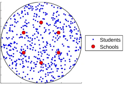
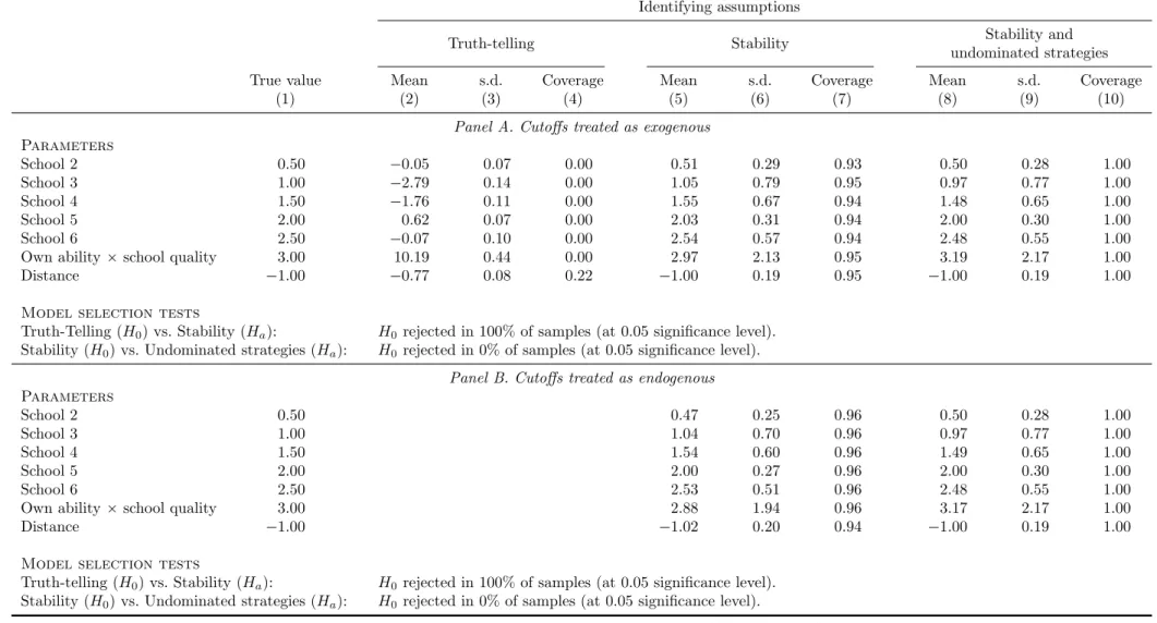
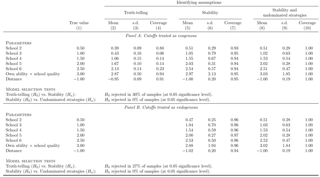
To validate the estimation approaches and tests, we carry out Monte Carlo (MC) simu-lations, the details of which are consigned to Appendix C.
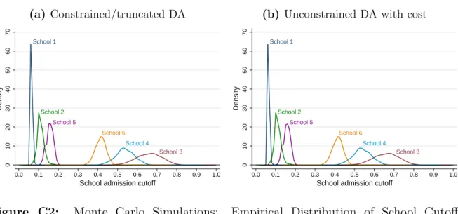
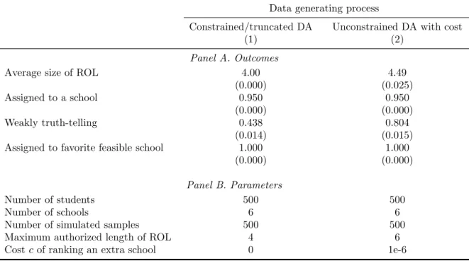
The Bayesian Nash equilibrium of the school choice game is simulated in two distinct settings where 500 students compete for admission into 6 schools. The first is the con-strained/truncated DA where students are allowed to rank up to 4 or 5 schools. The second setting, called the DA with cost, allows students to rank as many schools as they wish but imposes a constant marginal cost per additional school in the list.
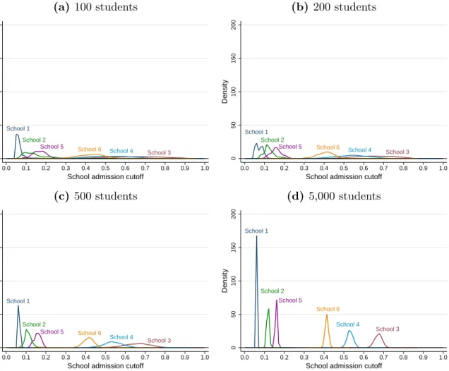
Several lessons can be drawn from these simulations. The first key result is that in both settings, the distribution of school cutoffs is close to jointly normal and degenerates as the number of seats and the number of students increase while holding constant the number of schools; the matching outcome is therefore “almost” stable (i.e., almost every student is assigned to her favorite feasible school) even in moderately-sized markets and with uncertainty in priority indices. By contrast, truth-telling is often violated by the majority of the students, even when they can rank 5 out of 6 schools (constrained DA) or when the cost of including an extra school is negligibly small (DA with cost). When the cost of ranking more schools becomes larger, the Bayesian Nash equilibrium of the game
can result in all students submitting fewer than 6 schools even when they are allowed to rank all of them. Based on these results, observing that only a few students make full use of their ranking opportunities cannot be viewed as a compelling argument in favor of truth-telling when cost is a legitimate concern.
A second important insight from the MC simulations is that the truth-telling estimates (ˆθT T) are severely biased. In particular, we note that students’ valuation of the most
popular schools tends to be underestimated, especially for students with low priority indices, because such schools are more likely to be omitted from their ROLs due to their low chance of admission. This bias is also present among small schools, which are often left out of ROLs because their admission cutoffs tend to be higher than than those of equally desirable but larger schools.
By contrast, the stability estimates (ˆθST) are reasonably close to the true parameter
values, whether cutoffs are endogenized or not, but their standard errors are larger than those obtained under truth-telling. This efficiency loss is a direct consequence of restrict-ing the choice sets to feasible schools and ignorrestrict-ing the information content of ROLs. Under the assumption that the matching outcome is stable, the Hausman-test presented in Section 2.4 strongly rejects truth-telling in our simulations.
The estimates from the moment (in)equalities approach (ˆθM I), which incorporates
the over-identifying information contained in students’ ROLs, are also consistent. Com-pared with using stability alone, the inclusion of moment inequalities is informative to the extent that these inequalities define sufficiently tight bounds for the probability of a preference ordering over some pairs of schools. This is more likely when the constraint on the length of ROLs is mild and/or when the cost of ranking an extra school is low, since these situations increase the chances of observing subsets of schools being ranked by a large fraction of students. A limitation of this approach, however, is that the cur-rently available methods for conducting inference based on moment (in)equality models are typically conservative. As a result, the marginal confidence intervals based on mo-ment (in)equalities tend to be wider than those obtained using momo-ment equalities alone, although the point estimates are closer to the true parameter values.
3
School Choice in Paris
Since 2008, the Paris Education Authority assigns students to public high schools based on a version of the school-proposing DA called AFFELNET (Hiller and Tercieux, 2014). Towards the end of the Spring term, final-year middle school students who are ad-mitted to the upper secondary academic track (Seconde G´en´erale et Technologique)20
are requested to submit a ROL of up to 8 public high schools to the Paris Education Authority. Students’ priority indices are determined as follows:
(i) Students’ academic performance during the last year of middle school is graded on a scale of 400 to 600 points.
(ii) Paris is divided into four districts. Students receive a “district” bonus of 600 points for each school in their list that is located in their home district, and no bonus for the others. Therefore, students applying to a school in their home district have full priority over out-of-district applicants to the same school.
(iii) Low-income students are awarded an additional bonus of 300 points. As a result, these students are given full priority over all other students from the same district.21
The DA algorithm is run at the end of the academic year to determine school assign-ment for the following academic year. Unassigned students can participate in a secondary round of admissions by submitting a new ROL of schools among those with remaining seats, the assignment mechanism being the same as for the main round.
3.1
Data
For our empirical analysis, we use data from Paris’ Southern District (Sud) and study the choices of 1,590 within-district middle school students who applied for admission to the district’s 11 public high schools for the academic year starting in 2013. Owing to the 600-point “district” bonus, this district is essentially an independent market.22 Moreover,
within the district, student priority indices are not school-specific, since all schools rank
20In the French educational system, students are tracked at the end of the final year ofcoll`ege (equiv-alent to middle school), at the age of 15, into vocational or academic upper secondary education.
21The low-income status is conditional on a student applying for and being granted the means-tested low-income financial aid in the last year of middle school. A family with two children would be eligible for this financial aid in 2013 if its taxable income was below 17,155 euros. The aid ranges from 135 to 665 euros per year.
22Out-of-district applicants could affect the availability of school seats in the secondary round, but this is of little concern since in the district, only 22 students out of 1,590 are unassigned at the end of the main round (for the comparison of assigned and unassigned students, see Appendix Table E6).
all students in the same way. The school-proposing DA is therefore equivalent to the student-proposing DA.
Along with information on socio-demographic characteristics and home addresses, our data contain all the relevant variables to replicate the matching outcome, including the schools’ capacities, the students’ ROLs of schools and their priority indices (converted into percentile ranks between 0 and 1). Individual examination results for the Diplˆome national du brevet (DNB)—a national exam that all students take at the end of middle school—are used to construct different measures of academic ability (math, French, and composite score), which are normalized as percentile ranks between 0 and 1.23
Table 1 reports students’ characteristics, choices, and admission outcomes. Almost half of the applicants are high socioeconomic status (SES), while 15 percent receive the low-income bonus. 99 percent are assigned to a within-district school in the main admission round, but only half obtain their first choice. Compared to their assigned schools, applicants’ first-choice schools tend to have higher ability and more socially privileged students.
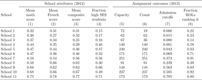
More detailed summary statistics for the 11 academic-track high schools in the district are presented in Table 2. Columns 1–4 show that there is a high degree of stratification among schools, both in terms of the average ability of students enrolled in 2012 and of their social background (measured by the fraction of high SES students). Columns 5–8 report a number of outcomes from the 2013 round of assignment. The district’s total capacity (1,692 seats) is unevenly distributed across schools: the smallest school has 62 seats while the largest has 251. Admission cutoffs in 2013 are strongly correlated with the different measures of school quality, albeit not perfectly. The last column shows the fraction of ROLs in which each school appears. The least popular three schools are ranked by less than 24 percent of applicants, and two of them remain under-subscribed (Schools 1 and 3) and thus have cutoffs equal to zero. Consistent with our Monte Carlo results, we note that small schools are omitted by many students, even if they are of high quality (e.g., School 8). Likewise, a sizeable fraction of students (20 percent) do not rank the highest-achieving school (School 11) in their lists.
23See Appendix B for a detailed description of the data sources. A map of the district is provided in Appendix Figure E4.
Table 1: High School Applicants in the Southern District of Paris: Summary Statistics
Variable Mean SD Min Max N
Panel A. Student characteristics
Age 15.0 0.4 13 17 1,590 Female 0.51 0.50 0 1 1,590 French score 0.56 0.25 0.00 1.00 1,590 Math score 0.54 0.24 0.01 1.00 1,590 Composite score 0.55 0.21 0.02 0.99 1,590 high SES 0.48 0.50 0 1 1,590
With low-income bonus 0.15 0.36 0 1 1,590
Panel B. Choices and outcomes
Number of choices within district 6.6 1.3 1 8 1,590
Assigned to a within-district school 0.99 0.12 0 1 1,590
Assigned to first choice school 0.56 0.50 0 1 1,590
Panel C. Attributes of first choice school
Distance (km) 1.52 0.93 0.01 6.94 1,590
Mean student French score 0.62 0.11 0.32 0.75 1,590
Mean student math score 0.61 0.13 0.27 0.78 1,590
Mean student composite score 0.61 0.12 0.31 0.77 1,590
Fraction high SES in school 0.53 0.15 0.15 0.71 1,590
Panel D. Attributes of assigned school
Distance (km) 1.55 0.89 0.06 6.94 1,577
Mean student French score 0.56 0.12 0.32 0.75 1,577
Mean student math score 0.54 0.14 0.27 0.78 1,577
Mean student composite score 0.55 0.13 0.31 0.77 1,577
Fraction high SES in school 0.48 0.15 0.15 0.71 1,577
Notes: This table provides summary statistics on the choices of middle school students from the Southern District of Paris who applied for admission to the district’s 11 public high schools for the academic year starting in 2013, based on
administrative data from the Paris Education Authority (Rectorat de Paris). All scores are from the exams of theDiplˆome
national du brevet(DNB) in middle school and are measured in percentiles and normalized to be inr0,1s. The composite
score is the average of the scores in French and math. The correlation coefficient between French and math scores is 0.50.
School attributes, except distance, are measured by the average characteristics of students enrolled in each school in the previous year (2012).
Table 2: High Schools in the Southern District of Paris: Summary Statistics
School attributes (2012) Assignment outcomes (2013) Mean math score Mean French score Mean composite score Fraction high SES students
Capacity Count Admission cutoffs Fraction ROLs ranking it School (1) (2) (3) (4) (5) (6) (7) (8) School 1 0.32 0.31 0.31 0.15 72 19 0.000 0.22 School 2 0.36 0.27 0.32 0.17 62 62 0.015 0.23 School 3 0.37 0.34 0.35 0.16 67 36 0.000 0.14 School 4 0.44 0.35 0.39 0.46 140 140 0.001 0.59 School 5 0.47 0.44 0.46 0.47 240 240 0.042 0.83 School 6 0.47 0.46 0.46 0.32 171 171 0.069 0.71 School 7 0.58 0.54 0.56 0.56 251 251 0.373 0.91 School 8 0.58 0.66 0.62 0.30 91 91 0.239 0.39 School 9 0.68 0.62 0.63 0.66 148 148 0.563 0.83 School 10 0.68 0.66 0.67 0.49 237 237 0.505 0.92 School 11 0.75 0.78 0.77 0.71 173 173 0.705 0.80
Notes: This tables provides summary statistics on the attributes of high schools in the Southern District of Paris and on
the outcomes of the 2013 assignment round, based on administrative data from the Paris Education Authority (Rectorat de
Paris). School attributes in 2012 are measured by the average characteristics of the schools’ enrolled students in 2012–2013.
All scores are from the exams of theDiplˆome national du brevet(DNB) in middle school and are measured in percentiles
and normalized to be inr0,1s. The composite score is the average of the scores in French and math. The correlation
3.2
Estimation and Test Results
Similar to Section 2, we assume that student i’s utility from attending school s can be represented by the following random utility model:
ui,sθsdi,s Xi,s1 β σi,s, s1, . . . ,11; (5)
whereθsis the school fixed effect,di,sis the distance to schoolsfromi’s place of residence,
andXi,sis a vector of student-school-specific observables. As observed heterogeneity,Xi,s
includes two variables that capture potential non-linearities in the disutility of distance and control for potential behavioral biases towards certain schools: “closest school” is a dummy variable equal to one if s is the closest to student i among all 11 schools; “high school co-located with middle school” is another dummy that equals one if high school s
and the student’s middle school are co-located at the same address.24 To account for
students’ heterogeneous valuations of school quality, interactions between student scores and school scores are introduced separately for French and math, as well as an interaction between own SES and the fraction of high SES students in the school. We normalize the variables inXi,sso that each school’s fixed effect can be interpreted as the mean valuation,
relative to School 1, of a non-high-SES student who has median scores in both French and math, whose middle school is not co-located with that high school, and for whom the high school is not the closest to her residence.
The idiosyncratic error term i,s is assumed to be an i.i.d. type-I extreme value, and
the variance of unobserved heterogeneity isσ2multiplied by the variance of
i,s. The effect
of distance is normalized to 1, and, therefore, the fixed effects and βare all measured in terms of willingness to travel. As a usual position normalization, θ1 0. We do not
consider an outside option because almost all students enroll in one of the 11 schools.25
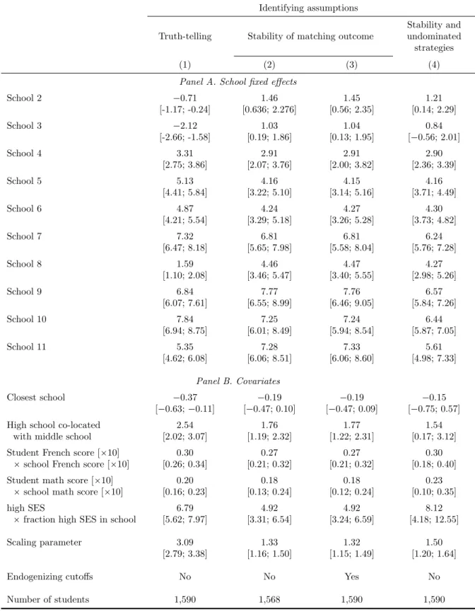
Using the same procedures as in the Monte Carlo simulations (described in Ap-pendix C), we obtain the results summarized in Table 3, where each column shows es-timates under a given identifying assumption: (i) truth-telling (column 1); (ii) stability with and without endogenizing the cutoffs (columns 2 and 3, respectively); and (iii) sta-bility with undominated strategies (column 4).26 Endogenizing the cutoffs in the last
24There are five such high schools in the district. 25
case does not make any difference, so we report only the estimates without endogenizing the cutoffs to save space.27
The results make evident that the truth-telling estimates (column 1) are rather dif-ferent from the others. More specifically, the “small-school” downward bias is apparent: 69 percent of students do not include School 8 in their ROLs due to the school’s small capacity (91 seats); the truth-telling assumption dictates that School 8 is less desirable than all the schools included in one’s ROL, which leads to a low estimation of its fixed effect. This under-estimation disappears when the model is estimated under the other two sets of assumptions. Similarly, there is a noticeable difference in the quality estimate of School 11, which is one of the most popular schools.
The Hausman test rejects truth-telling in favor of stability (p-value 0.01); the test based on moment (in)equalities does not reject the null hypothesis that stability is consistent with undominated strategies at a 5 percent significance level. The results in columns 2 and 3 are very similar, indicating that the market may be large enough for us to treat the cutoffs as exogenous. In the following, we focus on the results from columns 3 and 4.
The results show that “closest school” has no significant effect, but students signif-icantly prefer co-located schools. Compared with low-score students, those with high French (math) scores prefer more schools with higher French (math) scores. Moreover, high SES students prefer schools that have admitted a larger fraction of high SES stu-dents.
It is worth noting that the truth-telling estimates of the covariates (Panel B) are not noticeably different from our preferred ones. However, one cannot conclude that the truth-telling assumption produces reasonable results, as the estimates of fixed effects have shown. Moreover, the results of goodness of fit measures reported in Appendix D show that our preferred estimates fit the data well, as opposed to those based on truth-telling, whose predictions are far off the observed outcomes.
inequalities are constructed as described in Section 2.5. Determined by our selection ofXi,s, we interact
French score, math score, and distances to Schools 1 and 2 with the conditional moments. Although one could use more variables, e.g., SES status and distance to other schools, they provide only little additional variation.
27In principle, the assumption of undominated strategies alone implies partial identification (see Sec-tion 2.6). Because stability is not rejected by our test, we do not present results based on this approach (they are available upon request).
Table 3: Estimation Results under Different Identifying Assumptions
Identifying assumptions
Truth-telling Stability of matching outcome
Stability and undominated strategies
(1) (2) (3) (4)
Panel A. School fixed effects
School 2 0.71 1.46 1.45 1.21 [-1.17; -0.24] [0.636; 2.276] [0.56; 2.35] [0.14; 2.29] School 3 2.12 1.03 1.04 0.84 [-2.66; -1.58] [0.19; 1.86] [0.13; 1.95] [0.56; 2.01] School 4 3.31 2.91 2.91 2.90 [2.75; 3.86] [2.07; 3.76] [2.00; 3.82] [2.36; 3.39] School 5 5.13 4.16 4.15 4.16 [4.41; 5.84] [3.22; 5.10] [3.14; 5.16] [3.71; 4.49] School 6 4.87 4.24 4.27 4.30 [4.21; 5.54] [3.29; 5.18] [3.26; 5.28] [3.73; 4.82] School 7 7.32 6.81 6.81 6.24 [6.47; 8.18] [5.65; 7.98] [5.58; 8.04] [5.76; 7.28] School 8 1.59 4.46 4.47 4.27 [1.10; 2.08] [3.46; 5.47] [3.40; 5.55] [2.98; 5.26] School 9 6.84 7.77 7.76 6.57 [6.07; 7.61] [6.55; 8.99] [6.46; 9.05] [5.84; 7.26] School 10 7.84 7.25 7.24 6.44 [6.94; 8.75] [6.01; 8.49] [5.94; 8.54] [5.87; 7.05] School 11 5.35 7.28 7.33 5.61 [4.62; 6.08] [6.06; 8.51] [6.06; 8.60] [4.98; 7.33] Panel B. Covariates Closest school 0.37 0.19 0.19 0.15 [0.63;0.11] [0.47; 0.10] [0.47; 0.09] [0.75; 0.57]
High school co-located 2.54 1.76 1.77 1.54
with middle school [2.02; 3.07] [1.19; 2.32] [1.22; 2.31] [0.17; 3.12]
Student French score [10] 0.30 0.27 0.27 0.30
school French score [10] [0.26; 0.34] [0.21; 0.32] [0.21; 0.32] [0.18; 0.40]
Student math score [10] 0.20 0.18 0.18 0.23
school math score [10] [0.16; 0.23] [0.13; 0.24] [0.12; 0.24] [0.10; 0.35]
high SES 6.79 4.92 4.92 8.12
fraction high SES in school [5.62; 7.97] [3.31; 6.54] [3.24; 6.59] [4.18; 12.55]
Scaling parameter 3.09 1.33 1.32 1.50
[2.79; 3.38] [1.16; 1.50] [1.15; 1.49] [1.20; 1.64]
Endogenizing cutoffs No No Yes No
Number of students 1,590 1,568 1,590 1,590
Notes: This table reports the estimates of model (5) for the Southern District of Paris, with the coefficient on distance
being normalized to1. All estimates are based on maximum likelihood except those reported in column 4, which are
based on moment equalities and inequalities. In brackets, we report the 95 percent confidence interval. “Endogenizing cutoffs” refers to the inclusion of the likelihood terms or moment conditions that are derived based on the asymptotic distribution of cutoffs. An alternative approach to column 4, which also endogenizes cutoffs, yields exactly the same results
4