Microstructural characterisation of pearlitic and complex phase steels using image analysis methods

(1)

Microstructural Characterisation

of Pearlitic and Complex Phase Steels

Using Image Analysis Methods

by

Xi Liu

A thesis submitted to The University of Birmingham

For the degree of DOCTOR OF PHILOSOPHY

Metallurgy and Materials Science School of Engineering The University of Birmingham January 2014

(2)

University of Birmingham Research Archive

e-theses repository

This unpublished thesis/dissertation is copyright of the author and/or third parties. The intellectual property rights of the author or third parties in respect of this work are as defined by The Copyright Designs and Patents Act 1988 or as modified by any successor legislation.

Any use made of information contained in this thesis/dissertation must be in accordance with that legislation and must be properly acknowledged. Further distribution or reproduction in any format is prohibited without the permission of the copyright holder.

(3)

University of Birmingham Research Archive

e-theses repository

This unpublished thesis/dissertation is copyright of the author and/or third parties. The intellectual property rights of the author or third parties in respect of this work are as defined by The Copyright Designs and Patents Act 1988 or as modified by any successor legislation.

Any use made of information contained in this thesis/dissertation must be in accordance with that legislation and must be properly acknowledged. Further distribution or reproduction in any format is prohibited without the permission of the copyright holder.

(4)

Acknowledgements

A big thank you must go to my supervisors Dr R. M. Ward and Dr M. Strangwood, for all their guidance, encouragement, kind support and help throughout this project.

I would like to thank Professor P. Bowen for the provision of research facilities within the School of Metallurgy and Materials. Thanks are also given to all the staff and students that helped me during my time in the department.

Thanks to all the colleagues in the research group and my friends at the university. You make me really enjoy my 4 year time in Birmingham.

(5)

Abstract

The properties of materials are a primary factor to determine their applications, which makes the measurement of properties very important for both material design and quality control. As materials’ properties are determined by the microstructure of the materials such as grain size or the volume fraction of the present phases, microstructural characterisation is a powerful tool for property prediction.

Unfortunately, microstructural characterisation has not been widely applied with all steels such as pearlitic steels or complex multi-phase steels due to their complex microstructures. These microstructures may contain features that cannot be resolved by optical microscopy, and in which important information is contained in their texture rather than simply their grey level. These microstructures were investigated in this study using image texture analysis.

Fourier transform-based analysis was applied to pearlitic microstructures to extract the image orientation information. The orientation information as well as the grey value of low pass filtered image was used as predicates in a split-merge algorithm to segment the pearlitic colonies.

A supervised classification method based on various statistical measures including a number of 2-point statistics (Grey Level Co-occurrence Matrix measures) was developed to distinguish the bainite (upper bainite and lower bainite), martensite and ferrite phases in steels. The influence of etching on the analysis results was also investigated.

The pearlite colony segmentation was fairly accurate on a synthetic image that contains idealised pearlitic structures, but it was also found that there are fundamental difficulties with estimating colony boundaries from a real single 2-D pearlitic image. The multi-phase analysis was found to be fairly accurate for overall phase fraction under the conditions investigated here.

The investigation of etching effect on image analysis show that the method used in this study is not very sensitive to the etching degree.

(6)

Chapter 1. General Introduction

Steel has been one of the most important materials used by humans for up to 4000 years due to its good mix of properties and low cost. It has been found that the mechanical properties of steel are extremely dependent upon its internal structure at scales of nanometres up to microns or even millimetres (its ‘microstructure’). We can adjust the internal structure of steels through composition changes, heat treatments or mechanical deformation, and through this we can design them to fulfil various requirements in a range of applications.

There are multiple ways in which the atoms within steel can be arranged and bonded, called phases. Different phases have different properties, which may be suitable for different applications, either singly or in combinations. For instance pearlitic steels have high strength, good wear resistance and good delamination resistance (Krauss, 2005), so they are widely used as rail steels (Stone and Knupp, 1978, Bramfit et al., 1995) and steel wire (Krauss, 2005). The steels with more than one phase including dual phase steels, transformation induced plasticity steels and complex steels usually have good combination of strength and toughness, thus they are well suited for applications requiring strength and formability typically as in the automotive industry (Romero et al., 2010, Sodjit and Uthaisangsuk, 2012).

Whether a material is appropriate for a particular application is determined by the properties of the material. The properties can be measured using a range of mechanical tests, e.g. hardness, tensile, compressive and fatigue testing; chemical and physical tests. Some of the tests are readily accessible such as hardness. Others are difficult to measure such as yield or tensile strength as special samples have to be machined. Properties such as toughness and the fatigue strength are even more difficult to determine since the testing needs several samples for each condition and

(12)

2 the testing process is time-consuming.

Apart from by the above direct mechanical or physical tests, the properties of materials can also usually be predicted by characterising the microstructure of the materials, as the properties are determined by the microstructure. There are a number of microstructural characterisation techniques including optical microscopy, Scanning Electron Microscopy (SEM), Transmission Electron Microscopy (TEM), x-Ray Diffraction (XRD), Electron Backscattered Diffraction (EBSD), Magnetic-based methods and Ultrasonic sound based methods. Among these techniques, electron microscopy and optical microscopy are able to reveal the morphology of the microstructural features in a prepared sample surface. Electron microscopy is widely used due to its high resolution down to the nanometre scale. However optical microscopy also has its own advantages such as low cost, easy use on large sample areas and easy operability.

Specifically for the pearlitic steels, interlamellar spacing, colony size and prior austenite size are the factors that predominantly determine the strength and toughness properties (Gladman et al., 1972). For the interlamellar spacing measurement, a SEM or TEM is adequate. However to measure the colony size and especially the prior-austenite grain size is very difficult and requires a skilled metallographer using the light microscope or SEM and special procedures (Bramfitt, 1998). For the steels with multiple phases, the fraction, size, shape and distribution of the phase constituents determine the properties. XRD is an efficient technique to measure the fraction of the present phases, but the size, shape and distribution are not accessible. Image analysis methods are also applied for this application. Unlike the XRD technique, which is a crystallographic analysis of the bulk microstructure, image analysis method is extracting information directly from the micrograph of the sample surface. So once the present features in the sample images are classified into phases, the fraction, size, shape and distribution of these phases are easily obtained. Most of

(13)

3

the current image analysis based characterisation uses the histogram of the brightness (intensity) of the individual pixels that make up the image, and relies on all the pixels in one phase having intensities in a different range from all of those in another phase. This makes it extremely simple to distinguish the phases just using thresholding, and has been shown to work for some dual phase steels that have a high inter-phase contrast (Krebs et al., 2011, Burikova and Rosenberg, 2009). However for many other steels with more complex microstructures the different phases overlap in brightness levels. In this case, intensity thresholding is no longer able to distinguish the phases, and instead some analysis of the spatial patterns of intensity within the phases, the ‘texture’, is needed.

The aim of this PhD is to explore what is possible using texture-based optical image analysis methods for the two examples of: (1) colony characterisation of pearlitic steels and (2) phase classification of multi-phase steels.

(1) The difficulty that lies in the first task is that a pearlite colony contains two phases (ferrite and cementite) so it is not directly characterisable by the contrast of the phases; instead the orientation (and other features) of the lamellae determines a colony. This study needs to solve several problems: the measurement of the orientation of image pixels, the determination of appropriate features that characterise colonies and the segmentation of colonies using these features. A FFT based technique was used here to measure the orientation. A split and merge algorithm was applied for the image segmentation based on three features: orientation within a region, Kernel Average Misorientation along the interface between two adjacent regions and smoothed grey level within a region. The algorithm showed high accuracy on a synthetic image containing idealised lamellar structures. For images with real pearlitic structures, the results were less accurate because of the complexity of real pearlitic lamellae and the imperfections contained in the pearlitic structure apart from lamellae. However, no published literature could be found in this field, and so the work in this PhD shows

(14)

4 what is possible using an FFT-based technique.

(2) A quantitative analysis of some simple dual-phase steel microstructures, such as ferrite and martensite alone, can be carried out using conventional image analysis methods based on grey scale segmentation (characterising phases by the brightness of their individual pixels in an optical image). However for multi-phase steels with mixed microstructures containing small features and low inter-phase contrast, grey-scale segmentation is typically not applicable. Instead, image texture analysis can make use of the local patterns of variation in intensity between a pixel and its neighbours. Among a number of image texture analysis methods, those based on Grey Level Occurrence Matrix (GLCM) are widely used due to their general good performance in similar studies (refer to section 3.4.3). It was also applied in this study. The texture analysis method used here was ‘trained’ on regions of known phases that were manually selected from given images: firstly the neighbourhood size and other GLCM parameters were determined; then the best combination of 2-order statistical features, from a library of over 20, was determined using a Sequential Backward Selection algorithm. Finally those parameters were used to classify the images. Manual classification was also carried out as an evaluation of the automatic method. For a complex microstructure containing ferrite, martensite, upper and lower bainite, the manual classification results by different people varied greatly, which indicated the difficulty of the problem. The automatic classification result was mostly within the range of manual results. The algorithm was also used on a series of samples that have similar microstructures containing bainite and martensite. It showed high accuracy with those microstructures. Also the results indicated that the same set of features can be applied to similar microstructures without re-applying the feature selection procedure.

Image quality is a crucial factor in image analysis. In the particular application of material science, sample preparation is a primary influencing process to image quality.

(15)

5

Therefore it is important to study external influencing factors to image analysis results such as the degree of etching. For example if the only way to obtain accurate results from image analysis is by extremely careful etching, then it limits the broad application of the technique. If the results are fairly insensitive to the degree of etching, however, then the method can be widely used with confidence. The effects of etching were studied in this work, and found to be acceptable within practical limits.

(16)

6

Chapter 2. Literature Review on Steel Metallurgy, Microstructure

and Properties

2.1 Brief Background of Steel

Steel is an iron-based material containing low amounts of carbon and various additional alloying elements. It can be made into a great number of compositions with exactingly designed properties to meet a wide range of needs.

The earliest iron artefacts, from the 5th millennium BC in Iran and 2nd millennium BC in China, were made from meteoritic iron-nickel (Photos, 1989). The earliest known production of steel is a piece of ironware excavated from an archaeological site in Anatolia (Kaman-Kalehoyuk) and is about 4,000 years old. Although steel had been produced by various inefficient methods long before the Renaissance (roughly from the 14th century to the 17th century), it became a more common and inexpensive mass-produced material after more-efficient production methods were devised in the past few centuries, such as the Bessemer process and basic oxygen steelmaking, which lowered the cost of production while increasing the quality of the metal. Today, steel is one of the most common materials in the world (and iron is one of Earth’s most abundant elements), with more than 1.5 billion tons produced annually (WordsteelAssociation, 2012). It is a major component in buildings, infrastructure, tools, ships, automobiles, machines, appliances and weapons.

Nowadays, high and ultra-high strength steels are on the market with a tensile strength of up to 5500 MPa (Bhadeshia and Honeycombe, 2006). Other properties such as fracture toughness, weldability and ductility are specified for different applications.

(17)

7

The strength requirements may be met by adjustment of the chemical composition, mechanical processing and heat treatment through (i) work hardening, (ii) grain refinement, (iii) solid solution strengthening by interstitial and/or substitutional atoms, (iv) precipitation hardening (Bhadeshia and Honeycombe, 2006) and (v) transformation hardening.

2.2 Strengthening Mechanisms

2.2.1 Work Hardening

Work hardening, also known as strain hardening or cold working, is the phenomenon whereby a metal becomes harder and stronger as it is plastically deformed at temperatures lower than one third (typically) of the absolute melting temperature of the metal (Callister, 2007). Due to the increase of dislocation density (resulting from dislocation multiplication or the formation of new dislocations) with cold deformation, the average distance of separation between dislocations decreases, which means the resistance to dislocation movement by other dislocations becomes more significant. Thus the imposed stress necessary to continue plastic deformation of a metal increases with increasing cold work. However, work hardening is usually accompanied by a decrease in ductility.

2.2.2 Grain Refinement

Most materials for structural components are in the polycrystalline state, in which the grain size or the grain boundary density influences the mechanical properties significantly. Two main reasons cause grain boundaries to act as a barrier to dislocation motion (Callister, 2007):

a) A moving dislocation needs to change its direction to pass from one grain into another if the boundary between these two grains is low angle or a twin boundary; it

(18)

8

becomes more difficult as the misorientation between grains increases.

b) It is nearly impossible for a dislocation to move directly across high-angle grain boundaries due to a high misalignment of the boundaries. Stress at the end of dislocations piled-up at a grain boundary may trigger dislocations in adjacent grains, to move / from which will lead to a discontinuity of slip planes across the grains.

The grain boundary area to hinder dislocation motion is greater for smaller grains than for bigger grains. The grain size-strength relationship was firstly proposed by Hall (1951) and Petch (1953) as the following equation:

_{(Eq2.1) (Hall,}

1951, Petch, 1953)

Here d is the average grain diameter, and and k are constants for a particular material, is the yield stress.

However, the Hall-Petch relation is not valid any longer when grain boundaries make contributions to deformation by sliding and/or diffusive flow along the boundaries, which are independent of dislocation glide (Blum et al., 2006). A critical grain size ( ), below which the Hall-Petch relationship is no longer possible, is suggested as:

(Eq2.2) (Nieh and Wadsworth, 1991)

Where is the shear modulus, is the Burgers vector, is the Poisson’s ratio and is the material hardness.

(19)

9

2.2.3 Solid Solution Strengthening

This hardening technique is to alloy with impurity atoms that dissolve into the parent metal either substitutionally or interstitially. For iron only a few of elements such as carbon, hydrogen and nitrogen have atoms that are small enough to go into solution interstitially. The atoms of size and electronic structure close to those of iron, that do not combine to form carbides, nitrides, or other compounds, will substitute for iron atoms in iron crystals and form a substitutional solid solution.

The size and electronic structure differences between host iron atoms and either interstitial or substitutional alloying atoms impose lattice strains or stress fields that restrict the movement of dislocations. In the substitutional case, the stress fields are spherically symmetric, meaning that they have no shear stress component. Conversely, solute atoms in interstitial positions cause a tetragonal distortion, producing a shear field that can interact with edge, screw and mixed dislocations. A larger stress is needed to propagate the dislocation in any direction, which means a greater strengthening effect compared with the substitutional case (Krauss, 2005).

2.2.4 Precipitation Hardening and Dispersion Hardening

The hardening using second phase particles is commonly used for steels which normally have more than one phase present. For steels this would usually be carbo-nitrides or intermetallics (maraging steels) precipitated from solid solution.

When dislocations are moving through a matrix, which is precipitation hardened there are two main interactions. The dislocation can either cut through the particles or bend around and bypass them. The cutting of particles is possible only when the slip plane is continuous from the matrix through the precipitate particle.

(20)

10

precipitate particles in either cutting or bypassing cases. Orowan et al. (1954) proposed that in the bypassing case the dislocation is assumed to bend between two particles; yielding occurs when the bowed-out dislocation becomes semi-circular in shape; after yielding, the dislocation leaves Orowan loops around the particles, the formation of which makes the dislocation motion more and more difficult (Figure 2- 1).

The strength increase depends not only on the volume fraction of precipitates but also on their diameter and therefore the spacing or number density respectively. For a constant volume fraction of precipitates the material strength increases as the size of precipitates decreases.

Figure 2- 1 A schematic representation of Orowan mechanism for dispersion hardening (R.E.Smallman and A.H.W.Ngan, 2007)

2.2.5 Transformation Hardening

One of the significant advantages of iron is its allotropy, i.e. the prevailing crystal structure depends on composition, temperature and external pressure (Callister, 2007). At atmospheric pressure, there are three allotropic forms of iron: alpha iron (ferrite), gamma iron (austenite) and delta iron. The vast majority of steels rely on just two

(21)

11

allotropes, alpha and gamma. The crystal structure of pure iron changes from the body-centred cubic (bcc) to face-centred cubic (fcc) form during heating up at 910 °C (Ae3 point) (Bhadeshia and Honeycombe, 2006).

One of the reasons why there is a great variety of microstructures in steels is that the same allotropic transition can occur in a variety of ways depending on the manner in which the atoms move to achieve the change in crystal structure. The transformation can occur either by breaking of bonds and rearranging the atoms into an alternative pattern (reconstructive or diffusional transformation), or by inhomogeneously deforming the original pattern into a new crystal structure (displacive or shear transformation) (Bhadeshia and Honeycombe, 2006).

The diffusion of atoms leads to the new crystal structure during a reconstructive transformation. The flow of matter is sufficient to avoid shear components of the shape deformation. Displacive transformations occur at temperatures where diffusion is incompatible with the rate of transformation.

The allotropic property of iron makes the transformation hardening or phase balancing an important strengthening method for steel. Phase balance hardened steels use predominately higher levels of alloying elements, such as C and Mn, along with heat treatment to increase strength. Manganese increases hardenability and tensile strength of steel, but to a lesser extent than carbon. Mn is also able to decrease the critical cooling rate during hardening, thus increasing the steel’s hardenability much more efficiently.

Transformation-hardened steels can have a dual or triple microstructure of ferrite with varying levels of pearlite, bainite or martensite, which allows for varying levels of strength. Three basic types of transformation-hardened steels are dual-phase steels (DP), transformation-induced plasticity steels (TRIP) and martensitic steels.

(22)

12

The dual phase steels (ferrite and martensite) are often cast into slabs and hot rolled. Hot rolled coils are cold reduced and then further processed using continuously annealing technology.

TRIP steels consist of three phases: ferrite, bainite and retained austenite. It has been shown, that during the deformation process of an austenitic steel at ambient temperature the austenite steadily transforms into martensite, resulting in an increased elongation value (Kim, 1988). This combination of microstructures has the benefits of higher strength and great improvements in formability over other high-strength steels. Thermal processing for TRIP steels involves annealing the steel in the alpha + gamma region for some time and then quenching it to a point above the martensite start temperature, which allows the formation of bainite.

Martensitic steels are fully quenched to martensite during processing. The martensite structure is then tempered back to the appropriate strength level in order for adding toughness to the steel.

2.2.6 Effects of Carbon

Differences in the ability of ferrite and austenite to accommodate carbon result in important characteristics of the Fe-C diagram. The maximum solubility of carbon in austenite reaches 2.11wt% at 1148 °C. Ferrite has a much lower ability to dissolve carbon than austenite: the solubility reaches a maximum of only 0.02 wt% at 727 °C. The difference in solubility results from larger interstices in austenite. When the solubility limit for carbon in austenite or ferrite is exceeded, a new phase – iron carbide or cementite – forms in iron-carbon alloys and steels. Cementite crystals assume many shapes, arrangements, and sizes that together with ferrite contribute to the great variety of microstructures found in steels (Krauss, 2005).

(23)

13

2.3 Phases in Steel

2.3.1 Pearlite

Pearlite, as a lamellar mixture of ferrite and iron carbide, is a very common constituent of a wide variety of steels, where it provides a substantial contribution to strength.

When austenite is cooled, pearlite forms below the eutectoid temperature by the coordinated transform:

(Eq2.3) (Callister, 2007)

For carbon atoms to selectively partition to the cementite phase, diffusion is necessary (Figure 2- 2). The layered pearlite forms without long-range atomic diffusion but only with short range interfacial redistribution.

Figure 2- 2 Schematic representation of the formation of pearlite from austenite; direction of carbon diffusion indicated by arrows (Callister, 2007)

(24)

14

The true morphology of pearlite is sometimes not evident in two-dimensional sections. In three-dimensions, pearlite consists of an interpenetrating bi-crystal of cementite and ferrite, which when sectioned gives the lamellar appearance as can be seen in Figure 2- 3 (Bhadeshia and Honeycombe, 2006).

Figure 2- 3 Pearlite in a furnace-cooled Fe-0.75C alloy. Picral etch. Original magnification at 500x (Krauss, 2005)

Figure 2- 4 schematically illustrates the individual constituents of pearlite (however there is a mistake in the diagram: the colonies are not likely to cross prior austenite boundaries). A nodule nucleates at a grain boundary, triple point, grain corner, or surface inhomogeneity such as an inclusion and grows radially until impingement occurs with surrounding nodules (Bramfitt and Marder, 1973a). The basic structural

(25)

15

unit of pearlite is the colony. A nodule usually consists of an aggregate of more than one colony. Ideally pearlitic colonies are composed of parallel lamellae of cementite and intergrown ferrite (Garbarz and Pickering, 1988). Hull and Mehl’s work (1942) showed that all the ferrite lamellae had the same crystallographic orientation, and so did all the cementite lamellae. The joint growth of neighbouring colonies leads to a rounded nodule of pearlite (Guy and Hren, 1974).

Figure 2- 4 Schematic diagram illustrating the various constituents in the pearlitic microstructure (Elwazri et al., 2005)

Then a colony can be defined as a structural unit in which cementite lamellae are aligned nearly parallel to each other and pearlite nodule can be defined as a structural unit in which the ferrite matrix has nearly the same crystallographic orientation everywhere (Garbarz and Pickering, 1988). It was also found that in most cases a misorientation of the order of several degrees exists between pearlite colonies within one nodule (Walentek et al., 2006). Also, growth faults such as linear discontinuities in the cementite lamellae, deviations in the lamellae’ orientation, and low angle boundaries in the pearlitic ferrite usually occur in real pearlitic colonies (Bramfitt and

(26)

16 Marder, 1973b).

Colonies of lamellae of various orientations and spacings characterise the microstructure. However, the observed spacing on the optical micrograph is generally greater than the true lamellar spacing because the sectioning angle varies with respect to the lamellae plane (Samuel, 1999, Krauss, 2005), as is illustrated in Figure 2- 5.

Figure 2- 5 Surface topography of pearlite after etching (Samuel, 1999)

The true lamellar spacing has been studied by researchers and it is found that the spacing varies over wide ranges from 140 nm to 1900 nm (Mehl and Hagel, 1956, Ridley, 1984). The spacing is determined by a number of factors within which the subcritical temperature at which a colony is nucleated is prominent (Samuel, 1999).

Apart from the interlamellar spacing (in mm) of ferrite and cementite lamellae in pearlite, S, the prior austenite grain size (in mm), d, and pearlite colony size (in mm),

(27)

17

P, are also important influencing factors to the properties (Gladman et al., 1972). The Yield Strength (YS) of fully pearlitic steels can be expressed as:

(Eq2.4) (Hyzak

and Bernstein, 1976, Gladman et al., 1972)

The ductile-brittle Transition Temperature (TT) can be approximated from the following relationship:

(Eq2.5) (Hyzak

and Bernstein, 1976, Park and Bernstein, 1978)

From Eq2.4 and 2.5, it can be seen that for pearlite, strength is controlled by interlamellar spacing, colony size and prior-austenite grain size, and toughness is controlled by colony size and prior-austenite grain size. Unfortunately, all of these factors are difficult to measure. For the interlamellar spacing, a SEM or a TEM with a magnification of 10,000x is adequate. The colony size and especially the prior-austenite grain size are very difficult to measure and require a skilled metallographer using the light microscope or SEM and special procedures (Bramfitt, 1998).

Due to its high carbon content and other strengthening mechanisms including microalloying or cold work, pearlitic steels can achieve tensile strengths up to 4000MPa (Lesuer et al., 1996). Pearlite exhibits a good resistance to wear because of the hard carbide and some degree of toughness as a result of the ferrite’s ability to flow in an plastic manner (Li et al., 2005). Due to the excellent wear resistance along with good weldability, strength, and fracture resistance, pearlitic steels have been widely applied in industrial applications such as high-strength wires (Tarui et al., 1996,

(28)

18

Lesuer et al., 1996), structural applications (Lee et al., 2010), and especially the rail industry (Bolton and Clayton, 1984, Nakkalil et al., 1991, Garnham and Davis, 2011).

2.3.2 Bainite

Similar to pearlite in constitution, bainite also consists of ferrite and carbide (Borgenstam and Hillert, 1996). Often the transformation of austenite to bainite occurs in two stages, beginning with a displacive reaction which stops prematurely, to be followed by precipitation of carbides from the supersaturated ferrite or austenite at a slower rate (Bhadeshia, 2001).

Mainly depending on the transformation temperature and alloy composition (Mehl, 1939), there are two types of bainite formed: upper bainite, which is normally generated between 550 °C and 400 °C, and the other one is lower bainite, with a transition temperature range of 400 — 250 °C.

Lower bainite (lath bainite or plate bainite (Kutsov et al., 1999)), which is obtained by transformation at relatively low temperatures just above the martensite start temperature, consists of ferrite in a lath or plate and contains an intra-ferritic distribution of carbide particles (see Figure 2- 6) because of the slower diffusion rate associated with the reduced transformation temperature. Upper bainite (feathery bainite) forms at a higher temperatures and comprises a series of parallel ferrite laths separated by continuous or semi-continuous carbide layers or carbide-particle arrays (Figure 2- 6) (Bhadeshia, 2001, Yang and Fang, 2005).

(29)

19

Figure 2- 6 Schematic representation of the transition from austenite to upper or lower bainite (Bhadeshia, 2001)

Both of these consist of aggregates of ferrite plates, which are called sheaves, separated by cementite, martensite or untransformed austenite. The plates within each sheaf are called sub-units (Figure 2- 7).

Many observations showed that the shape of a sheaf is that of a wedge-shaped plate (Srinivasan and Wayman, 1968). The thicker end of the wedge usually begins at an austenite grain boundary. The sub-units within sheaves have a lenticular plate or lath morphology.

The thickness of bainite plates is determined by the austenite strength, phase transformation driving force and transformation temperature (only a small effect) as shown in Figure 2- 8 (Bhadeshia, 2001). Strong austenite and high driving force lead to thicker bainite plates. Statistics show that the value of thickness can range from 50 nanometres to 340 nanometres (Singh and Bhadeshia, 1998, Bhadeshia, 2001).

(30)

20

Figure 2- 7 (a) Light micrograph illustrating sheaves of lower bainite in a partially transformed (395°C) Fe- 0.3C- 4Cr wt% alloy. The light etching matrix is martensite. (b) Corresponding transmission electron micrograph illustrating sub-units of lower bainite (Bhadeshia, 2001)

Figure 2- 8 The significance of each of the variables plotted on the horizontal axis (temperature, driving force and austenite strength), in influencing the thickness of bainite plates (Bhadeshia, 2001)

Generally bainitic steels are stronger and harder than pearlitic steels because of their finer structure (Figure 2- 9). The mechanical properties also vary with the

(31)

21

morphology of bainite. The tensile strength is higher for bainite obtained at lower transformation temperatures than for higher transformation temperatures due to the finer plate size and higher dislocation density (Bhadeshia, 2001).

Figure 2- 9 Variation in the tensile strength of structural steels as a function of the temperature at which the rate of transformation is greatest during continuous cooling heat treatment (Irvine et al., 1957)

The property-microstructure relationship becomes more complicated when the toughness of bainitic steels is considered. The spacing of high angle boundaries in the bainitic structure is particularly important in this case, as the high-angle boundaries impede the propagation of cleavage cracks. Thus, that is the coarsest carbides in the microstructure which control toughness of the steel. The presence of comparatively large carbides in bainite, especially upper bainite, leads to a decrease in toughness (Barbacki, 1995).

2.3.3 Martensite

(32)

22

quenched) to a relatively low temperature. At the martensite formation temperature, diffusion, even of interstitial atoms, is usually not conceivable over the time of the experiment. Therefore the chemical composition of the martensite is identical to that of the parent austenite.

During the displacive lattice transformation from FCC of austenite to BCT of martensite, the interstitial space for the accommodation of carbon atoms (diameter: 0.154 nm) decreases from 0.1044 nm to 0.0346 nm, which produces a big distortion in the BCC lattice (Pan et al., 1998). The deformation of the austenite lattice causes a change in the shape of the transformed region, consisting of a large shear and a volume expansion (Bhadeshia and Honeycombe, 2006). The displacive transformation can be described as two successive shear displacements - first by a homogeneous shear throughout the plate which occurs parallel to a specific plane in the parent phase known as the habit plane. The second displacement is inhomogeneous by one of two mechanisms: slip as in Fe-C martensite or twinning as in Fe-Ni martensite (Figure 2- 10).

Mainly dependent on the carbon content, three types of martensite can be formed during quenching. The morphology of low carbon (up to 0.5 wt%) martensite is lath-like. For lath martensite the laths have an average thickness about 200 nm (Lee et al., 2009), and a length ranging from several to dozens of microns (Kotrechko et al., 2006). Lath martensite has a fuzzy and nondistinct appearance, as shown in Figure 2- 11. The medium carbon martensite, with characteristic morphology is that of lenticular plates (Figure 2- 12), first start to form in steels with about 0.5 wt% carbon. Unlike the laths, the lenticular plates form in isolation rather than in packets. When the carbon content is higher than 1.4 wt%, the orientation relationship and the habit plane of martensite changes but the morphology is still lenticular plates (Bhadeshia and Honeycombe, 2006). In plate martensite, it is possible to see the individual plates.

(33)

23

Figure 2- 10 The phenomenological theory of martensite crystallography RB: the combination of Bain strain B and rigid body rotation R, is a invariant-line strain, P1 and P2 are invariant-plane strain (Bhadeshia and Honeycombe, 2006)

(34)

24

Figure 2- 12 Optical micrograph of plate martensite from a 1.4% C steel (Verhoeven, 2007)

It appears that there are two main contributions to the high strength of martensite (Cohen, 1962). One comes from the structures of twin plates or high dislocation density (Kelley and Nutting, 1961); the other one is that the carbon atoms strain the ferrite lattice, due to the increase of distortion during quenching as mentioned above (Dieter, 1988).

The microstructures of martensite and bainite at first seem quite similar like thin plates (Sandvik, 1982, Swallow and Bhadeshia, 1996, Dunne and Wayman, 1971); this is a consequence of the two microstructures sharing many aspects of their transformation mechanisms. Under a simple light microscope, the microstructure of bainite appears darker than martensite since there is a larger phase contrast effect with the ferrite/carbide interfaces in bainite than that with the lath boundaries in martensite (Bowen et al., 1986). Also, the particle size in bainite is much coarser than that in martensite (Tarpani et al., 2002, Wei et al., 2004), as is shown in the example in Figure 2- 13 and Table 2- 1.

(35)

25

Figure 2- 13 Microstructure of the bainite/martensite double-phase steel (Shah, 2013)

Table 2- 1 Some microstructural characterisations of martensite and bainite (Bowen et al., 1986)

Microstructure Mean cementite

size/nm

Coarsest particle/nm Tempered martensite (tempering: usually

performed by reheating and cooling after hardening process)

38 110

Auto-tempered martensite (the tempering of the first-formed martensite, i. e. the martensite formed near Ms, during the reminder of the quench)

14 36

Upper bainite 220 1000

Mixed upper and lower bainite 230 720

Of the various microstructures that may be produced for a given steel alloy, martensite is the hardest and strongest and the most brittle. Its hardness is dependent on the carbon content as demonstrated in Figure 2- 14. In contrast to pearlitic steels, strength and hardness of martensite are attributed to the effectiveness of the interstitial carbon atoms in hindering dislocation motion (as a solid-solution effect) and to the relatively few slip systems rather than to the microstructure.

(36)

26

Figure 2- 14 Hardness (at room temperature) as a function of carbon concentration for plain carbon martensitic, tempered martensitic, and pearlitic steels (Bain, 1939, Grange et al., 1977, Callister, 2007)

2.4 Effects of Mixed Microstructures on Properties

Conventional high strength steels are manufactured by adding alloying elements such as Nb, Ti, V, and/or P in low carbon or IF (interstitial free) steels. These steels have widely been applied. However, as the demands for weight reduction are further increased, new families of high strength steels including DP (dual phase), TRIP (transformation induced plasticity), FB (ferrite-bainite), CP (complex phase) and TWIP (twin induced plasticity) steels have been developed (Zrnik et al., 2006).

Due to an excellent combination of strength and ductility and relative ease of manufacture, dual phase steels having two phases namely ferrite and martensite are gaining the widest industrial usage especially in the automotive industry (Romero et al., 2010, Sodjit and Uthaisangsuk, 2012). The hard second phase of martensite is

(37)

27

present in the form of islands in a matrix of ferrite. The property of good ductility to this steel is imparted by the soft ferrite phase, which is generally continuous.

The microstructure of transformation-induced plasticity steels (TRIP steel), consists of ferrite, bainite and metastable austenite (Jacques et al., 2001). During deformation, whether in forming or during operation, the retained austenite transforms into a harder phase – martensite – providing this material with enhanced work-hardening characteristics (Jingyi et al., 2011). The TRIP effect is also thought to be the main phenomenon responsible for the improved balance of strength and ductility exhibited by the new and so-called “TRIP-assisted multiphase steels” (Stringfellow et al., 1992).

Complex phase steels belong to a group of steels with very high tensile strength of 800 MPa or even greater. The chemical composition of CP steels, and also their microstructure, is very similar to that of TRIP steels. Typically, CP steels have no retained austenite in the microstructure, but contain harder phases such as martensite and bainite (Kuziak et al., 2008).

High strength structural steels with mixed microstructure of martensite, bainite and ferrite have been found to have better strength and toughness than single phase microstructures of low temperature products. Generally speaking, the strength and hardness of steel increase with increasing martensite volume fraction; while the ductility decreases. This is valid for both triple phase steels (ferrite, bainite and martensite) (Zare and Ekrami, 2011) and dual phase steels (ferrite and martensite) (Erdogan and Tekeli, 2002). At the same martensite volume fraction values, fine microstructures demonstrated a better combination of strength and ductility and higher hardness than coarse ones (Erdogan and Tekeli, 2002). The presence of bainite (typically lower bainite) in steels contributes to the improvement of toughness. However, there is not a monotonic relationship between them. Bohlooli and Nakhaei

(38)

28

(2013) compared the strength and ductility of three bainite-ferrite steels containing 49%, 54% and 63% bainite respectively. The results showed the sample with 63% bainite had the highest strength and best ductility. However, when the bainite fraction increased to 100%, its toughness and ductility decreased greatly (Saeidi and Ekrami, 2009).

Tomita and Okabayashi (1985) concluded that the mechanical properties, especially toughness, of high strength steels having a mixed microstructure of martensite and bainite are affected more by the size, shape, and distribution of bainite rather than the difference in martensite and bainite strength, and/or the type of mixture present. In the steel with a multiple phase microstructure they tested, the occurrence of upper bainite resulted in poor toughness (Tomita and Okabayashi, 1985, Tomita and Okabayashi, 1983). Also they found that for that steel a mixed microstructure containing tempered martensite with 25% lower bainite provided the best combination of strength and ductility. These findings were confirmed by Abbaszadeh et al. (2012) and Young and Bhadeshia (1994) using martensite-bainite dual phase steels. They also observed a maximum point (at about 28% bainite) in the curve of strength as a function of lower bainite fraction. They explained this phenomenon (strength increase first as increasing the lower bainite fraction from a fully martensitic structure) on the basis of two factors: a) the partitioning of the prior austenite grains by the lower bainite resulting in the refinement of martensite substructures (Tomita and Okabayashi, 1983); b) the strengthening of the lower bainite by the surrounding relatively rigid martensite because of a plastic constraint effect. Abbaszadeh et al. also found that the increasing of the upper bainite volume fraction in the mixed upper bainite-martensite microstructures resulted in the decreasing of properties such as yield strength, ultimate tensile strength, elongation and Charpy V-notch impact energy.

Therefore, it is important to measure the fraction of phase constituents in a mixed microstructure (including distinguishing upper and lower bainite), in order to

(39)

29 predicate the properties of the material.

2.5 Quantitative Characterisation of Microstructure

The determination of the properties of samples is essential for the development of new materials with specifically tailored properties, the design of their thermomechanical treatments and the quality control of existing fabrication processes.

Some mechanical properties are readily accessible, such as hardness. Others are difficult to measure such as yield or tensile strength, as special samples have to be machined from the material. Properties such as toughness and the fatigue strength are far more difficult to determine since the testing needs several samples for each condition and the testing process is time-consuming.

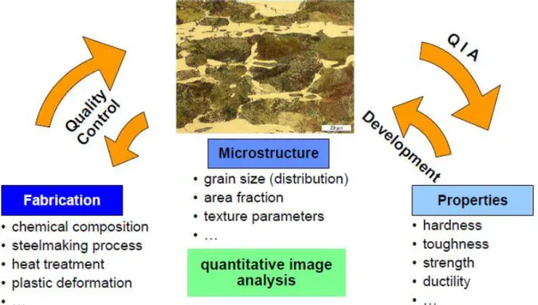
In many systems, relationships between properties and microstructure have been established, e.g. the Hall-Petch relationship (Hall, 1951), as microstructures have been more readily obtained than mechanical data and contain a large amount of information about the materials and their processing history. Quantitative analysis of microstructural images not only allows the possibility of performing a quality control check of the processing route, but also gives the possibility of further establishing correlations between microstructural features and related properties (Figure 2- 15).

(40)

30

Figure 2- 15 Microstructure as a connection between the fabrication of components and their properties (Fuchs, 2005)

However, particularly for strengthening mechanisms, the relevant microstructural features have various scales and techniques for being quantitatively analysed. The grain size of steels or the morphological units of phases (e.g. bainitic laths) have a scale of micrometres, so they can be characterised with optical microscopy or scanning electron microscopy; the strengthening precipitates or second phases can range from nanometres (e.g. nitrides or intermetallic compounds) to micrometres (e.g. carbides), so can also be characterised with SEM or possibly optical microscopy; the solid solution strengthening is to dissolve alloying elements in to parent atoms substitutionally or interstitially, while work hardening is to produce more dislocations with the material, both of which are only observable with TEM and hard to characterise. Therefore, among the strength influencing factors, only the grain size and phase balance can be characterised optically.

(41)

31

Chapter 3. Literature Review on Image Analysis

3.1 Background of Digital Image Analysis

3.1.1 Microscopy and Image Acquisition

The material structures as reviewed in Chapter 2 have to be magnified for viewing and analysis due to their size. Traditionally, optical microscopy is commonly used in this field of characterisation. The resolution of an optical microscope is dependent on the wavelength of light used to image the sample surface and can be calculated according to

(Eq3.1)

(Hecht, 2002, Jonkman et al., 2003)

Where represents the resolution limit, denotes the wavelength of the light, n the refractive index of the medium between object and objective and the angle between the illuminating beam and the optical axis of the microscope. N.A. is also referred to as numerical aperture.

For the medium air n has a value of about 1. This means that the resolution of an optical microscope is limited to about 476 nm for red light with a wavelength of about 780 nm. The spatial resolution of an optical microscope is often given an approximate value of 0.35 μm. Compared to the typical sizes of the features of the phases (martensite, bainite) that reviewed in section 2.3.3, it can be found that the martensite laths are not resolvable under optical microscope, while lower and upper bainite may be resolvable.

(42)

32

necessary. This can be achieved using electron microscopy. Thanks to the very small wavelength of the electron (around 0.5 nm for an accelerating voltage of 60 kV) compared to the wavelength of the optical light, 100000 times the resolution of the optical microscope should be achievable theoretically (Fuchs, 2005).

Nevertheless optical microscopy plays an important role in quantitative image analysis due to its advantages over electron microscopes:

- lower price

- greater availability in both scientific and industrial environments - comparatively simple usability

- additional information from colour images - possibility of high automation

- lower requirements for sample preparation

Thanks to these strengths, optical microscopy is still widely used in both scientific and industrial environments in spite of its disadvantage of limited resolution. However as some aspects of the microstructure which would allow phases too be simply characterised cannot be resolved optically, alternative methods have to be found to characterise the optical images of the complex microstructures of modern steels.

3.1.2 Types of Digital Image Analysis

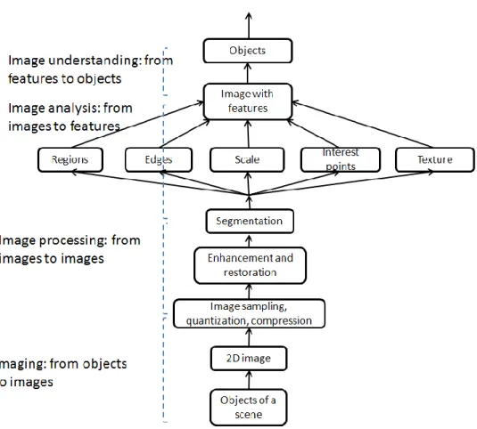
Image representation can be roughly divided into four levels (Figure 3- 1), or alternatively two even simpler ways are often distinguished: low-level image processing (transform of an image to another including image compression, pre-processing methods for noise filtering, edge extraction and image sharpening) and high-level image interpretation (Sonka et al., 1998). E.g. the inputs are images, but the outputs are a set of characteristics or parameters (e.g. detecting the owner of a face or

(43)

33

finger print) extracted from those images (Gonzalez and Woods, 2007).

Figure 3- 1 Four possible levels of image representation suitable for image analysis problems (Sonka et al., 1998)

3.2 Image Shade Correction

3.2.1 Shading Problem in Image Acquisition

Optical microscope images are produced by the interaction between objects in real space, the illumination, and the camera. In the optical imaging system, the images frequently exhibit significant variation in intensity (shading) across the field-of-view. In some cases, the image may be brighter in the centre and darker in the edge; in other cases the brightness of the pixels on one side may be higher than those on the other. The shading might be attributed to multiple factors from non-uniform illumination, non-uniform camera sensitivity, the design of the light path between the camera and the microscope or even dirt and dust on glass (lens) surfaces (Rochow and Tucker,

(44)

34

1994). This shading effect is of great harm for subsequent image processing and especially quantitative image analysis, therefore eliminating it is frequently necessary.

Imaging system

The shading correction issue was studied and discussed by Young (2000). He theoretically described this problem. The illumination over the microscope field-of-view interacts with the object in a multiplicative way to produce the image :

(Eq3.2)

(Young, 2000)

The object represents various microscope imaging modalities:

(Eq3.3) (Young, 2000)

where OD(x,y) is the optical density, c(x,y) is proportional to the concentration of fluorescent material, and r(x,y) is the reflectance, which is applicable in this case. The camera also often contributes gain and offset terms, so that:

(Eq3.4) (Young, 2000)

(45)

35 contributing to the problem of shading.

3.2.2 Shading Correction Method

Two calibration images are needed through the imaging system – BLACK[m,n] and WHITE[m,n]. The BLACK image is generated by covering the lens leading to b(x,y) in shading model (Eq3.4) equal 0, which in turn leads to BLACK[m,n]=offset[m,n]. The WHITE image is generated by using a[m,n]=0 which gives . The correction then becomes:

(Eq3.5) (Young, 2000)

The constant term is chosen to produce the desired dynamic range. The same equation was also given by van den Doel et al. (1998) and a textbook written by Murphy (2001).

In the shading correction process of this study, the white image was taken from an as-polished sample and the black image was simply to set ‘0’ everywhere in the image.

3.3 Conventional Intensity Based Image Analysis

The intensity of image pixels, regardless of location, often carries much of the information about features (feature: a quantitative measure of a certain texture characteristic) in an image and so is most important for images analysis. Furthermore, intensity based approaches such as image thresholding and subsequent edge detection are effective and fast for the analysis of simple images.

(46)

36

global threshold. Then segmentation can be carried out by labelling each pixel as object or background depending on its intensity value compared with the threshold value.

Figure 3- 2 (a) Original image; (b) image histogram (Coste, 2012)

Figure 3- 2 (a) shows a simple image; Figure 3- 2 (b) shows its histogram. By simply applying a threshold as the local minimum value between two intensity peaks in Figure 3- 2(b), a segmented image can be obtained as Figure 3- 3.

(47)

37

Figure 3- 3 Segmented image of Figure 3- 2(a)

This technique is suitable for images that consist of objects with homogeneous intensities and definite contrast. However, many images are more complicated, so image texture analysis is induced and more widely applied nowadays.

3.4 Image Texture Analysis

All natural and artificial images have texture in common, which gives information not just about the colour or grey level of a point in an image, but also about the spatial arrangement of colour or intensities in an image or selected region of an image (Shapiro and Stockman, 2001). Figure 3- 4 gives an example of different textures: dog fur, grass, river pebbles, cork, checkered textile, and knitted fabric (Sonka et al., 1998).

(48)

38

Figure 3- 4 Textures: (a) dog fur; (b) grass; (c) river pebbles; (d) cork; (e) checkered textile; (f) knitted fabric (Sonka et al., 1998)

The main aim of texture analysis is texture recognition and texture-based shape analysis. Some more precise features in the tone and structure of a texture, rather than simply being described as fine, coarse, grained, smooth, etc, are needed to be found to make machine recognition possible (Sonka et al., 1998). For this four different approaches have been established (Materka and Strzelecki, 1998):

- geometrical (or structural) - statistical

(49)

39 - model-based

- signal processing (or transform) methods

For the structural approach texture is represented by well-defined primitives (the simplest geometric objects or shapes such as a point, a straight line or a cube) and a hierarchy of spatial arrangements of these primitives (Materka and Strzelecki, 1998). A structural description of a texture includes a set of identifiable primitives and a specification of their placement patterns (the probability of the chosen primitive being placed at a particular location (Materka and Strzelecki, 1998)), which needs to be efficiently computable. As the structural approaches are based on the theory that textures are made up of primitives appearing in a near-regular repetitive arrangement (Cun Lu and Yan Qiu, 2004), it can work well for man-made, regular patterns.

In contrast to structural methods, statistical approaches do not attempt to describe the exact structure of the texture (Cun Lu and Yan Qiu, 2004). They represent the texture indirectly by computing at each point in the image non-deterministic properties (or local features) that govern the distributions and relationships between the grey levels (Materka and Strzelecki, 1998) and deriving a set of statistics from the distributions of the local features (Ardizzoni et al., 1999). The autocorrelation (ACF) method (Haralick, 1979), edge frequency (EF) method (Haralick, 1979) and the well-known Grey Level Co-occurrence Matrix (GLCM) (Haralick et al., 1973) are classical statistical approaches to texture analysis.

Model-based texture analysis (Derin and Elliott, 1987, Manjunath and Chellappa, 1991) such as fractal dimension (Chaudhuri and Sarkar, 1995) and Markov Random Field (MRF) (Krishnamachari and Chellappa, 1997), using fractal and stochastic models, attempt to interpret an image texture by use of generative image and stochastic models respectively. It has been shown to be useful for texture analysis and discrimination (Kaplan and Kuo, 1995, Chaudhuri and Sarkar, 1995); however, it lacks orientation selectivity and is not suitable for describing local image structures

(50)

40

(Materka and Strzelecki, 1998). In addition, the computational complexity arising in the estimation of stochastic model parameters is another big problem.

Transform methods of texture analysis, such as Fourier (Chi-Ho and Pang, 2000), Gabor (Idrissa and Acheroy, 2002) and wavelet transforms (Arivazhagan and Ganesan, 2003), represent an image in a space whose co-ordinate system has an interpretation that is closely related to the characteristics of a texture (such as frequency or size). The usefulness of Gabor filters is limited in practice because there is usually no single filter resolution at which one can localise a spatial structure in natural textures (Osicka, 2008). The wavelet transforms feature several advantages over Gabor transform (Materka and Strzelecki, 1998):

- varying the spatial resolution allows it to represent textures at the most suitable scale,

- there is a wide range of choices for the wavelet function.

They make wavelet transforms attractive for texture segmentation, however the problem of being not translation-invariant still exists (Lam and Li, 1997).

3.4.1 Approaches of Estimating the Local Orientation of Images

Numerous techniques for estimating the local orientation or anisotropy of images have been developed so far. Rao (1990) introduced an approach to determine the principal orientation field of an image using the direction of local grey-level gradients. The Principal Component Analysis (PCA) (for explanation see (Pearson, 1901)) of local grey level gradient based method is also popular (Bazen et al., 2000). The 2-dimensional probability density function of the gradient vectors can be obtained by performing the PCA to the auto-covariance matrix of them. And the main direction of gradient can be measured from the auto-covariance matrix. This technique has been applied for fingerprint segmentation (Bazen and Gerez, 2002) in which the researchers used PCA to estimate the directional field from the gradients of grey level, and measure the orientation of the fingerprint by extracting the singular points where

(51)

41

the directional field is discontinuous. This method provided same results as the traditional method but it was not capable of detecting low-quality areas in a fingerprint.

Gu et al. (2004) improved the technique for the orientation field of fingerprints using a combination of two models including a polynomial model to approximate the orientation field globally and a point-charge model at each discontinuous or singular point. The two models were combined smoothly through a weight function. Experimental results showed that the method was more accurate and robust compared with the previous work.

However, most of the established methods including the methods shown above rely on the strong hypothesis that the gradients are well-defined, which make them very sensitive to noise (Bergonnier et al., 2007). The Fourier transform introduced below is also a powerful tool in measuring the local orientation of image. It is less sensitive to noise because the Fourier transform based methods do not measure the orientation directly by the location gray value gradients and also a noise removal operation can be easily performed based on the Fourier transform.

3.4.2 Fourier Transform (FT)

The Fourier transform is named in the honour of Joseph Fourier. Its basic concept is that any function of time or space that periodically repeats itself, or even functions that are not periodic (but whose area under the curve is finite), can be expressed as the sum of sine and/or cosine waves of different frequencies, each multiplied by a different coefficient (Gonzalez and Woods, 2007). Fourier transform has enormous applications in physics, engineering and chemistry, including communication (Gregory and Gallagher, 2002), image processing and data analysis.