Adaptive Beamforming Algorithm based on Generalized Opposition-based Simulated Kalman Filter

Adaptive Beamforming Algorithm based on

Generalized Opposition-based Simulated Kalman

Filter

Kelvin Lazarus

, Nurul Hazlina Noordin

, Kamil Zakwan Mohd Azmi

, Nor Hidayati Abdul Aziz

, and

Zuwairie Ibrahim

1

_{Faculty of Electrical and Electronics Engineering}

Universiti Malaysia Pahang

26600 Pahang, Malaysia

2

_{Faculty of Engineering and Technology}

Multimedia University

Jalan Ayer Keroh Lama

75450 Melaka, Malaysia

Abstract— In this paper, a new population-based metaheuristic optimization algorithm named Generalized Opposition-based Simulated Kalman Filter (GOBSKF) is proposed as adaptive beamforming algorithm. GOBSKF is an improved version of Simulated Kalman Filter (SKF). Adaptive beamforming algorithm based on GOBSKF is compared with previously published work which is Adaptive Mutated Boolean PSO (AMBPSO) and Minimum Variance Distortionless Response (MVDR) for different noise level. The results show that GOBSKF is proven to be better than AMBPSO and MVDR.

Keywords—Adaptive Beamforming; Generalized Opposition-based Simulated Kalman Filter

1.

I

Wireless communication system involves time-varying signal propagation environment where the user and interferers move around with time. Adaptive beamforming is used to adapt continuously to the changing electromagnetic environment by continuously adjusting the weights of individual elements in an array. In adaptive beamforming techniques, the main beam must be pointed towards the direction of the desired signal and nulling the interference at the same time.

Since adaptive beamforming is considered as an optimization problem, there are a number of optimization algorithms that were applied in adaptive beamforming application [1]–[22]. These algorithms are used to find the optimum weights so as to steer the main beam towards the signal of interest (SOI) and null the interference to maximize the signal to interference plus noise ratio (SINR) value.

In this paper, a new metaheuristic optimization technique named Generalized Opposition-based Simulated Kalman Filter (GOBSKF) is proposed for adaptive beamforming application. GOBSKF is an extended version of Simulated Kalman Filter (SKF). SKF is introduced by Ibrahim et. al. [23] and has been applied to solve various optimization problems [24]–[29]. Generalized Opposition-based Learning is one of many Opposition-Opposition-based Learning method used to improve optimization algorithm [30]. The main idea of Opposition-based Learning is to check the current solution continuously with the opposite solution within the search space in order to get a better approximation of current solution [31]. GOBSKF is used to estimate weights of individual elements in an array which gives the maximum signal to interference plus noise ratio (SINR) value.

2.

S

M

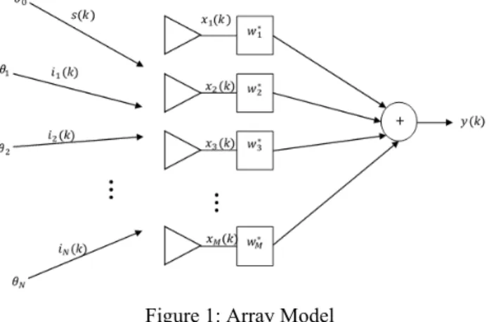
Assuming an array antenna of M elements and N number of interfering signal with signal of interest (SOI) of kth time sample, s(k), arriving at angle θ0, and signal not of interest (SNOI), i1(k), i2(k), i3(k), …, iN-1(k), iN(k), arriving at angle θ1, θ2, θ3, …, θN-1, θN, as

shown in Fig. 1 [32].

Figure 1: Array Model The array output, y(k) can be represented by

𝑦 𝑘 = 𝑤& _{∙ 𝑥(𝑘) (1)}

where 𝑤 stands for weights for individual elements, 𝐻 for Hermitian transpose and 𝑥 𝑘 is the signal vector. The signal vector 𝑥 𝑘 can be further expanded as

𝑥 𝑘 = 𝑎-𝑠 𝑘 + 𝑎0 𝑎1 ⋯ 𝑎3 ∙ 𝑖0 𝑘 𝑖1 𝑘 ⋮ 𝑖3 𝑘 + 𝑛 𝑘 = 𝑥7 𝑘 + 𝑥8 𝑘 + 𝑛(𝑘) (2)

where 𝑎8 stands for M-element array steering vector for 𝜃8 direction of arrival; 𝑥7(𝑘) is the desired signal vector, 𝑥7(𝑘) the

interference signal vector and with noise, 𝑛(𝑘). The total array output, 𝑦 𝑘 is expanded as

𝑦 𝑘 = 𝑤&_{∙ 𝑥}

7(𝑘) + 𝑥8(𝑘) + 𝑛(𝑘) = 𝑤&∙ 𝑥7+ 𝑢(𝑘) (3)

where the undesired signal, 𝑢 𝑘 is formulated as

𝑢 𝑘 = 𝑥₈ 𝑘 + 𝑛 𝑘 (4)

Next, the array correlation matrices are calculated for both desired signal, 𝑅77 and undesired signal, 𝑅<< . The weighted array output

power for desired signal, 𝜎71 is given as below

𝜎₇1_{= 𝐸 𝑤}&_{∙ 𝑥}

71 = 𝑤&∙ 𝑅77∙ 𝑤 (5)

where the signal correlation matrix, 𝑅₇₇, can be formulated as

𝑅77= 𝐸 𝑥7𝑥7& (6)

𝜎<1= 𝐸 𝑤&∙ 𝑢1 = 𝑤&∙ 𝑅<<∙ 𝑤 (7)

where the undesired correlation matrix, 𝑅<< is formulated as

𝑅<<= 𝑅88+ 𝑅?? (8)

with 𝑅88 denotes as the interference correlation matrix and 𝑅?? as noise correlation matrix.

The fitness function is the signal to interference plus noise ratio, SINR, can be formulated as [31]. GOBSKF will find the optimum weights, 𝑤 which give maximum SINR value.

𝑆𝐼𝑁𝑅 =𝜎7 1 𝜎<1= 𝑤&_{∙ 𝑅} 77∙ 𝑤 𝑤&_{∙ 𝑅} <<∙ 𝑤 (9)

3.

G

O

-

S

K

F

Generalized Opposition-based Simulated Kalman Filter (GOBSKF) is extended from the existing Simulated Kalman Filter (SKF). SKF is inspired by the estimation capabilities of Kalman Filter [23]. In SKF, each agent acts as an individual Kalman Filter. Consider 𝑡 as the number of iteration and 𝑁 number of agents, estimated solution of optimization problem of the 𝑖DE _{agent at a time 𝑡, 𝑿}

𝒊 𝒕 is defined as 𝑿_𝒊(𝑡) = 𝒙₈𝟏_{(𝑡), 𝒙} 𝒊 𝟐_{(𝑡), … , 𝒙} 𝒊 𝒅_{(𝑡), … , 𝒙} 𝒊 𝑫_{(𝑡) (10)}

where 𝒙𝒊𝒅(𝑡) is the estimated state of 𝑖DE agent in 𝑑DE dimension and 𝐷 is the maximum number of dimensions. In an iteration, 𝑡, all

the agents are involved in the calculation of fitness, and the agent with best fitness is identified as 𝑿𝒃𝒆𝒔𝒕(𝒕). SKF performs a simulated

measurement process to get to the true value, 𝑿_{𝒕𝒓𝒖𝒆}. The 𝑿_{𝒕𝒓𝒖𝒆} will update when better 𝑿_{𝒕𝒓𝒖𝒆} solution is found.

GOBSKF begins with random initialization of agents, 𝑿(𝟎), within the search space. The initial value for error covariance estimate, 𝑃(0), process noise, 𝑄 and the measurement noise, 𝑅, are defined at initial stage.

Iteration begins with fitness calculation of 𝑖DE _{agent, 𝑓𝑖𝑡}

8(𝑿(𝒕)). 𝑿𝒃𝒆𝒔𝒕(𝒕) is updated based on the type of problem. For minimization

problem,

𝑿𝒃𝒆𝒔𝒕(𝑡) = 𝑚𝑖𝑛8∈0,1,…,3𝑓𝑖𝑡8(𝑿(𝒕)) (11)

whereas, in maximization problem,

𝑿_{𝒃𝒆𝒔𝒕}(𝑡) = 𝑚𝑎𝑥_{8∈0,1,…,3}𝑓𝑖𝑡₈(𝑿(𝒕)) (12)

Later, 𝑿𝒕𝒓𝒖𝒆 will be updated when bettersolution is found (𝑿𝒃𝒆𝒔𝒕 𝑡 < 𝑿𝒕𝒓𝒖𝒆 for minimization problem or 𝑿𝒃𝒆𝒔𝒕 𝑡 > 𝑿𝒕𝒓𝒖𝒆 for

maximization problem).

In prediction process, the following time-update equations

𝑥8(𝑡|𝑡 + 1) = 𝑥8(𝑡) (13)

𝑃 𝑡|𝑡 + 1 = 𝑃 𝑡 + 𝑄 (14)

are used to make a prediction for the state and error covariance estimates given the prior estimates. The next step is measurement which acts as a feedback to the estimation process. The following equation simulates the measurement for each agent:

The final process is estimation. In this process, Kalman gain, 𝐾(𝑡), is computed as follows:

𝐾 𝑡 = 𝑃 𝑡|𝑡 + 1

𝑃 𝑡|𝑡 + 1 + 𝑅 (16)

After that, the measurement-update equations are used to improve the a posteriori estimates from the a priori estimates by making use of the measurement.

𝑥8(𝑡 + 1) = 𝑥8 𝑡 𝑡 + 1 + 𝐾 𝑡 ×𝑧8 𝑡 − 𝑥8 𝑡 𝑡 + 1 (17)

𝑃 𝑡 + 1 = (1 − 𝐾(𝑡))×𝑃 𝑡|𝑡 + 1 (18)

Using the measured position as feedback and influenced by the Kalman gain value, 𝐾 𝑡 , each agent updates an estimate of the optimum for that corresponding iteration.

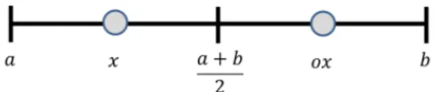
Fig. 2 shows the illustration of Opposition-based Learning where 𝑥 stands for current position and 𝑜𝑥 stands for opposite position in domain [a,b].

Figure 2: Opposite point, 𝑜𝑥, defined in domain [a,b]

The opposite population, 𝑥_𝑜𝑏8,n, is generated using equation 19, where 𝑥_𝑜𝑏8,n is the opposite solution for current solution, 𝑥8,n, in

domain [a,b], the 𝑟𝑎𝑛𝑑 is random numbers between -1 and 1, 𝑁 represents the number of agents, and 𝐷 is the number of dimensions.

𝑥_𝑜𝑏8,n = 𝑟𝑎𝑛𝑑 × 𝑎n+ 𝑏n − 𝑥8,n

𝑖 = 1,2, … 𝑁 ; 𝑗 = 1,2, … 𝐷

(19)

In GOBSKF, the opposite population is generated within the current population’s range as in equation 20 where 𝑀𝐼𝑁_nr _{and 𝑀𝐴𝑋} nr

represent the lowest and highest agent in the current population, respectively. The execution of opposite population generation depends on the value of jumping rate, Jr.

𝑥_𝑜𝑏8,n= 𝑟𝑎𝑛𝑑 × 𝑀𝐼𝑁nr+ 𝑀𝐴𝑋nr − 𝑥8,n

𝑖 = 1,2, … 𝑁 ; 𝑗 = 1,2, … 𝐷

(20)

If the generated opposite solution exceeds the converged search space, the opposite solution is reinitialized using equation 21.

𝑥_𝑜𝑏8,n= 𝑀𝐼𝑁nr+ 𝑟𝑎𝑛𝑑 × 𝑀𝐼𝑁nr− 𝑀𝐴𝑋nr

𝑖 = 1,2, … 𝑁 ; 𝑗 = 1,2, … 𝐷

(21)

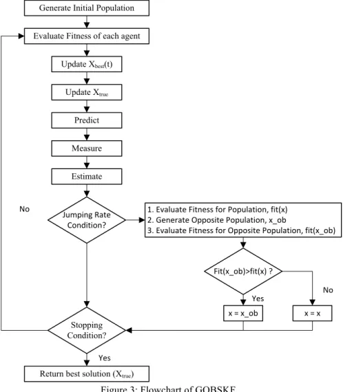
Generate Initial Population Evaluate Fitness of each agent

Update Xbest(t) Update Xtrue Predict Measure Estimate Stopping Condition?

Return best solution (Xtrue) Yes

No _{Jumping Rate}

Condition?

1. Evaluate Fitness for Population, fit(x) 2. Generate Opposite Population, x_ob

3. Evaluate Fitness for Opposite Population, fit(x_ob)

Fit(x_ob)>fit(x) ?

x = x_ob x = x

Yes No

Figure 3: Flowchart of GOBSKF

4.

E

S

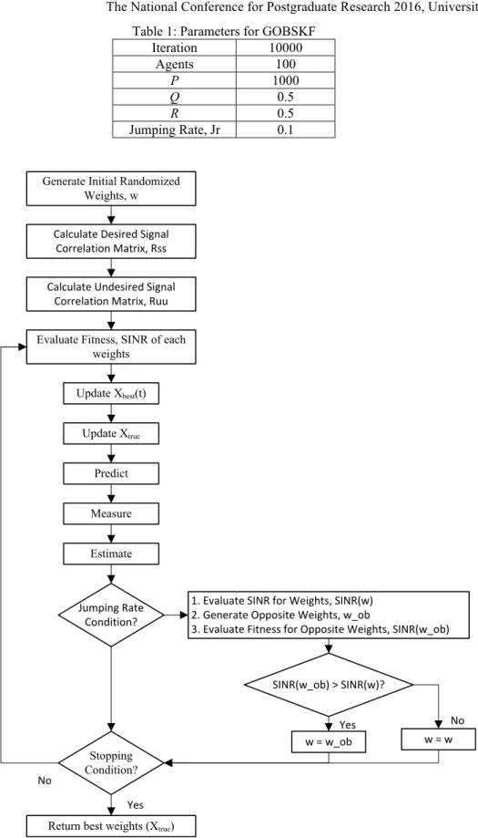
GOBSKF is applied to 10 elements uniform linear array antenna in the simulation. The distance between elements is set to 0.5 λ as its most commonly used distance. Table 1 shows the parameters used in GOBSKF. The desired angle is set to 30∘ _{and the interference}

angle is set to −70∘_{, −40}∘_{, −30}∘_{, −10}∘_{, 0}∘_{, 10}∘_{, 50}∘_{, and 70}∘ _{similar to the parameters established by Z.D. Zaharis and T.V. Yioultsis}

[1].

GOBSKF is used to find the optimum weights by maximizing SINR value. Fig. 4 shows the flowchart of GOBSKF in adaptive beamforming application. The performance of GOBSKF is compared with AMBPSO and MVDR [1]. The test was executed 100 times and a statistical analysis was performed.

5.

S

R

D

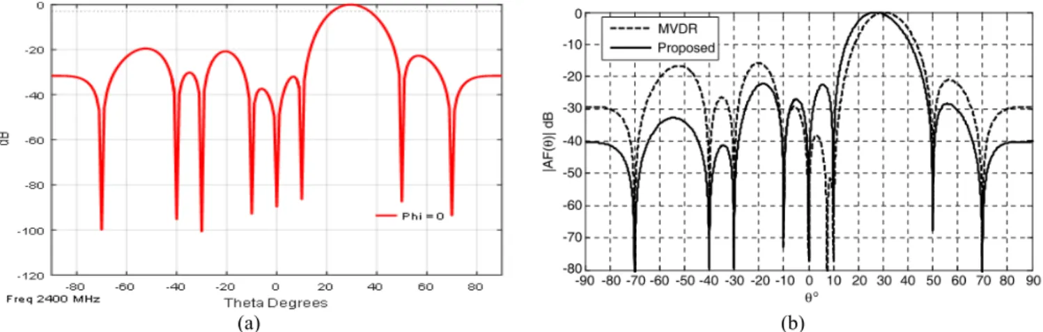
Fig. 5 shows the radiation pattern produced GOBSKF with a signal to noise ratio, SNR = 30 dB and is compared with radiation pattern obtained by Z.D. Zaharis and T.V. Yioultsis using conventional MVDR and AMBPSO [1]. The desired signal at 30- _{and the}

interference angle is set to −70∘_{, −40}∘_{, −30}∘_{, −10}∘_{, 0}∘_{, 10}∘_{, 50}∘ _{and 70}∘ _{just like the condition set in [1]. From Fig. 5, AMBPSO is}

able to produce much lower maximum sidelobe level compared with MVDR and GOBSKF, but GOBSKF is able to produce much deeper nulls compared to MVDR and AMBPSO. Statistical analysis is performed to confirm the results of GOBSKF is significant.

Table 1: Parameters for GOBSKF Iteration 10000 Agents 100 P 1000 Q 0.5 R 0.5 Jumping Rate, Jr 0.1

Generate Initial Randomized Weights, w

Evaluate Fitness, SINR of each weights Update Xbest(t) Update Xtrue Predict Measure Estimate Stopping Condition?

Return best weights (Xtrue)

Yes No

Jumping Rate Condition?

1. Evaluate SINR for Weights, SINR(w) 2. Generate Opposite Weights, w_ob

3. Evaluate Fitness for Opposite Weights, SINR(w_ob)

SINR(w_ob) > SINR(w)?

w = w_obYes w = w

No Calculate Desired Signal

Correlation Matrix, Rss Calculate Undesired Signal

Correlation Matrix, Ruu

Table 2 lists the results for GOBSKF compared with AMBPSO and also with conventional MVDR adaptive beamforming algorithm with various signal to noise ratio (SNR) values. GOBSKF is mostly able to produce much higher mean SINR values compared with the mean SINR of AMBPSO and also the SINR of MVDR. The SINR values for GOBSKF does not fluctuate much compared to AMBPSO because of its lower standard deviation, STD values.

Statistical analysis is also performed between MVDR and mean results for AMBPSO and GOBSKF using Friedman rank test. Table 3 shows the Friedman rank for GOBSKF, AMBPSO, and MVDR.

After that, Friedman PostHoc analysis is performed using Holm’s procedure. Table 4 shows the results obtained after performing Friedman PostHoc analysis. Holm`s procedure rejects those hypotheses that have a p-value ≤ 0.05. Therefore, there is a significant difference between GOBSKF and AMBPSO and also with MVDR.

(a) (b)

Figure 5: Radiation Pattern for SNR = 30dB: (a) GOBSKF; (b) MVDR and AMBPSO by Z.D. Zaharis and T.V. Yioultsis [1] Table 2: Comparison of SINR (dB) Values of MVDR, AMBPSO, and GOBSKF

Table 3: Friedman Ranking GOBSKF 1.1176 AMBPSO 1.8824

MVDR 3.0000

Best Worst Mean STD Best Worst Mean STD

-20 -10.0540 -10.0522 -10.0548 -10.0523 0.0004 -10.0522 -10.0522 -10.0522 0.0000 -15 -5.1601 -5.1395 -5.1512 -5.1399 0.0020 -5.1395 -5.1395 -5.1395 0.0000 -10 -0.3701 -0.2975 -0.3692 -0.2998 0.0098 -0.2975 -0.2976 -0.2975 0.0000 -5 4.3345 4.5321 4.3422 4.5269 0.0218 4.5321 4.5321 4.5321 0.0000 0 8.8967 9.4241 8.5481 9.3749 0.1643 9.4241 9.3888 9.4233 0.0050 5 13.4522 14.3768 12.0647 14.2676 0.3628 14.3768 14.2140 14.3708 0.0194 10 18.2011 19.3598 15.1371 19.2810 0.4463 19.3573 18.5395 19.2749 0.1142 15 22.6889 24.3542 16.5370 24.1008 1.0643 24.3466 23.4416 24.1327 0.1956 20 27.3035 29.3509 17.2416 29.0332 1.2290 29.3390 27.3695 28.9813 0.3147 25 31.7012 34.3515 22.4314 33.6680 1.4163 34.3468 32.8502 33.9586 0.3633 30 36.4811 39.3341 30.2715 38.7648 0.8722 39.3483 37.0333 38.8979 0.4563 35 40.4633 44.3440 32.6393 43.1564 1.5287 44.3508 42.0255 43.8573 0.4774 40 45.2813 49.3461 36.6898 48.1781 1.2409 49.3417 46.2094 48.8883 0.5595 45 49.3217 54.3358 43.2386 52.5134 1.5788 54.3477 51.7545 53.8767 0.4519 50 54.8269 59.3317 47.6499 58.3221 1.7439 59.3469 57.5601 58.9174 0.4195 55 59.1356 64.3458 52.7630 63.0660 1.6119 64.3500 61.0678 63.9052 0.5396 60 63.4345 69.3468 56.3379 67.5858 1.8369 69.3510 67.2908 68.8662 0.4599

Table 4: Friedman PostHoc Analysis

Data Set p z Holm MVDR vs GOBSKF 0.0000 5.4880 0.0167 MVDR vs AMBPSO 0.0011 3.2585 0.0250 AMBPSO vs GOBSKF 0.0258 2.2295 0.0500

6.

C

The main purpose of any adaptive beamforming algorithm is to improve the signal to interference plus noise ratio, SINR by steering the main beam towards the desired signal and null the undesired signal at the same time. With the ever changing electromagnetic environment, it also important that the adaptive beamforming algorithm efficiently adapt and maintain its maximum SINR value every time. Therefore, the proposed method, GOBSKF, is proven better compared to AMBPSO and also conventional MVDR. GOBSKF provided better mean SINR values and is also consistent. Results obtained by GOBSKF is also proven to be significant.

A

The authors will like to thank Universiti Malaysia Pahang for providing internal financial support through grant GRS1503120. This research is also supported by Fundamental Research Grant Scheme (FRGS) awarded to Multimedia University (FRGS-1-2015-TK04-MMU-03-2).

R

[1] Z. D. Zaharis and T. V Yioultsis, “A Novel Adaptive Beamforming Technique Applied on Linear Antenna Arrays Using Adaptive Mutated Boolean PSO,” Prog. Electromagn. Res., vol. 117, p. 15, 2011.

[2] S. K. Goudos, V. Moysiadou, T. Samaras, K. Siakavara, and J. N. Sahalos, “Application of a comprehensive learning particle swarm optimizer to unequally spaced linear array synthesis with sidelobe level suppression and null control,” IEEE Antennas Wirel. Propag. Lett., vol. 9, pp. 125–129, 2010.

[3] N. Dib, S. K. Goudos, and H. Muhsen, “Application of Taguchi’s optimization method and self-adaptive differential evolution to the synthesis of linear antenna arrays,” Prog. Electromagn. Res., vol. 102, pp. 159–180, 2010.

[4] K. Guney and M. Onay, “Bees algorithm for interference suppression of linear antenna arrays by controlling the phase-only and both the amplitude and phase,” Expert Syst. Appl., vol. 37, no. 4, pp. 3129–3135, 2010.

[5] V. Zuniga, A. T. Erdogan, and T. Arslan, “Control of Adaptive Rectangular Antenna Arrays using Particle Swarm Optimization,” Loughbrgh. Antennas Propag. Conf., no. November, pp. 385–388, 2010.

[6] L. Pappula and D. Ghosh, “Linear antenna array synthesis using cat swarm optimization,” AEU - Int. J. Electron. Commun., vol. 68, no. 6, pp. 540–549, 2014.

[7] K. Guney and S. Basbug, “Linear Antenna Array Synthesis Using Mean Variance Mapping Method,” Electromagnetics, vol. 34, no. 2, pp. 67–84, 2014.

[8] U. Singh, “Linear Array Synthesis Using Biogeography,” Prog. Electromagn. Res. M, vol. 11, pp. 25–36, 2010.

[9] T. S. Kiong, S. B. Salem, J. K. S. Paw, K. P. Sankar, and S. Darzi, “Minimum variance distortionless response beamformer with enhanced nulling level control via dynamic mutated artificial immune system,” Sci. World J., vol. 2014, 2014. [10] K. Najmy, A. Rani, M. Fareq, A. Malek, N. S. Chin, and A. A. Wahab, “Modified and Hybrid Cuckoo Search Algorithms

via Weighted – Sum Multiobjective Optimization for Symmetric Linear Array Geometry Synthesis,” vol. 3, no. 5, pp. 6774–6781, 2014.

[11] K. N. Abdul Rani, M. F. Abd Malek, and N. Siew-Chin, “Nature-inspired cuckoo search algorithm for side lobe suppression in a symmetric linear antenna array,” Radioengineering, vol. 21, no. 3, pp. 865–874, 2012.

[12] M. A. Zaman and M. Abdul Matin, “Nonuniformly spaced linear antenna array design using firefly algorithm,” Int. J. Microw. Sci. Technol., vol. 2012, 2012.

[13] O. Kaid Omar, F. Debbat, and A. Boudghene Stambouli, “Null steering beamformer using hybrid algorithm based on Honey Bees Mating Optimisation and Tabu Search in adaptive antenna array,” Prog. Electromagn. Res. C, vol. 32, no. July, pp. 65–80, 2012.

[14] S. Darzi, T. S. Kiong, M. T. Islam, M. Ismail, S. Kibria, and B. Salem, “Null Steering of Adaptive Beamforming Using Linear Constraint Minimum Variance Assisted by Particle Swarm Optimization, Dynamic Mutated Artificial Immune System, and Gravitational Search Algorithm,” Sci. World J., vol. 2014, no. 724639, p. 10, 2014.

[15] S. Darzi, S. K. Tiong, M. T. Islam, M. Ismail, and S. Kibria, “Optimal Null Steering of Minimum Variance Distortionless Response Adaptive Beamforming Using Particle Swarm Optimization and Gravitational Search Algorithm,” in 2014 IEEE

2nd International Symposium on Telecommunication Technologies (ISTT), Langkawi, Malaysia, 2014, pp. 230–235. [16] S.Pal, B.Y. Qu, S.Das, and P.N. Suganthan, “OPTIMAL SYNTHESIS OF LINEAR ANTENNA AR- RAYS WITH

MULTI-OBJECTIVE DIFFERENTIAL EVOLUTION,” Prog. Electromagn. Res. B, vol. 21, pp. 87–111, 2010.

[17] K. Guney and M. Onay, “Optimal synthesis of linear antenna arrays using a harmony search algorithm,” Expert Syst. Appl., vol. 38, no. 12, pp. 15455–15462, 2011.

[18] K. Guney and A. Durmus, “Pattern Nulling of Linear Antenna Arrays Using Backtracking Search Optimization Algorithm,”

Hindawi Publ. Corp. Int. J. Antennas Propag., vol. 2015, p. 10, 2015.

[19] C. Doroody, T. S. Kiong, and S. Darzi, “SINR Improvement Using Firefly Algorithm (FA) for Linear Constrained Minimum Variance (LCMV) Beamforming Technique,” no. I4ct, pp. 441–445, 2015.

[20] S. Darzi, M. T. Islam, S. K. Tiong, S. Kibria, and M. Singh, “Stochastic leader gravitational search algorithm for enhanced adaptive beamforming technique,” PLoS One, vol. 10, no. 11, p. 20, 2015.

[21] K. Kaur and V. K. Banga, “SYNTHESIS OF LINEAR ANTENNA ARRAY USING FIREFLY ALGORITHM,” Int. J. Sci. Eng. Res., vol. 4, no. 8, pp. 601–606, 2013.

[22] D. Mandal, N. T. Yallaparagada, S. P. Ghoshal, and A. K. Bhattacharjee, “Wide Null Control of Linear Antenna Arrays Using Particle Swarm Optimization,” in 2010 Annual IEEE India Conference (INDICON), 2010, pp. 2–5.

[23] Z. Ibrahim, N. H. A. Aziz, N. A. A. Aziz, S. Razali, M. I. Shapiai, S. W. Nawawi, and M. S. Mohamad, “A Kalman filter approach for solving unimodal optimization problems,” ICIC Express Lett., vol. 4, no. 5, pp. 1–8, 2015.

[24] Z. Md Yusof, Z. Ibrahim, I. Ibrahim, K. Z. Mohd Azmi, N. A. Ab Aziz, N. H. Abd Aziz, and M. S. Mohamad, “Angle modulated simulated kalman filter algorithm for combinatorial optimization problems,” ARPN J. Eng. Appl. Sci., vol. 11, no. 7, pp. 4854–4859, 2016.

[25] Z. Md Yusof, Z. Ibrahim, I. Ibrahim, K. Z. Mohd Azmi, N. A. Ab Aziz, N. H. Abd Aziz, and M. S. Mohamad, “Distance Evaluated Simulated Kalman Filter for Combinatorial Optimization Problems,” ARPN J. Eng. Appl. Sci., vol. 11, no. 7, pp. 4904–4910, 2016.

[26] B. Muhammad, Z. Ibrahim, K. H. Ghazali, K. Z. Mohd Azmi, N. A. Ab Aziz, N. H. Abd Aziz, and M. S. Mohamad, “A new hybrid simulated Kalman filter and particle swarm optimization for continuous numerical optimization problems,”

ARPN J. Eng. Appl. Sci., vol. 10, no. 22, pp. 17171–17176, 2015.

[27] Z. Yusof, I. Ibrah, and S. N. Satiman, “BSKF : Binary Simulated Kalman Filter,” in Third International Conference on Artificial Intelligence, Modelling and Simulation, 2015, pp. 77–81.

[28] Z. Md Yusof, S. N. Satiman, K. Z. Mohd Azmi, B. Muhammad, S. Razali, Z. Ibrahim, Z. Aspar, and S. Ismail, “Solving Airport Gate Allocation Problem using Simulated Kalman Filter,” Int. Conf. Knowl. Transf., 2015.

[29] A. Adam, Z. Ibrahim, N. Mokhtar, M. I. Shapiai, M. Mubin, I. Saad, “Feature selection using angle modulated simulated Kalman filter for peak classification of EEG signals,” SpringerPlus, Vol. 5, No. 1580, 2016.

[30] Q. Xu, L. Wang, N. Wang, X. Hei, and L. Zhao, “A review of opposition-based learning from 2005 to 2012,” Eng. Appl. Artif. Intell., vol. 29, pp. 1–12, 2014.

[31] H. R. Tizhoosh, “Opposition-Based Learning: A New Scheme for Machine Intelligence,” Comput. Intell. Model. Control Autom. 2005 Int. Conf. Intell. Agents, Web Technol. Internet Commer. Int. Conf., vol. 1, pp. 695–701, 2005.