Verification of Workflow Nets

Verification of Workflow Nets

Eindhoven University of Technology, P.O. Box 513, NL-5600 MB, Eindhoven, The Netherlands. [email protected]

Abstract. Workflow management systems will change the architecture of future informa-tion systems dramatically. The explicit representainforma-tion of business procedures is one of the main issues when introducing a workflow management system. In this paper we focus on a class of Petri nets suitable for the representation, validation and verification of these proce-dures. We will show that the correctness of a procedure represented by such a Petri net can be verified by using standard Petri-net-based techniques. Based on this result we provide a comprehensive set of transformation rules which can be used to construct and modify correct procedures.

1 Introduction

At the moment more than 250Workflow Management Systems(WFMSs) are available. This number signifies the importance of the workflow paradigm ([3,4,6,13,18,23]). Un-fortunately, today’s WFMSs suffer from a number of serious drawbacks. A theoretical basis for workflow management tools is missing. As a result there are, even at a concep-tual level, important differences between the tools. Despite the efforts of the Workflow Management Coalition [26] there are no real standards. Moreover, the absence of tools to support the analysis of workflows is a serious drawback for the success of today’s WFMSs. In this paper we present a Petri-net-based approach to overcome some of these problems. In particular we will address the problem of analyzing the correctness ofworkflow procedures.

Business processes supported by a WFMS are centered around procedures. A proce-dure is the method of operation used by a business process to process cases. Exam-ples of cases are orders, claims, travel expenses, tax declarations, etc. The procedure specifies the set of tasksrequired to process these cases successfully. Moreover, the procedure specifies the (partial) order in which these tasks have to be executed. The goal of a procedure is to handle cases efficiently and properly. To achieve this goal, the procedure should be tuned to the ever changing environment of the business process. A WFMS supports the definition and modification of procedures. Unfortunately, most of the WFMSs allow for the specification of incorrect procedures. We have evaluated many WFMSs. None of these WFMSs allow for the verification of essential properties such as the absence of deadlock and livelock.

In this paper we focus on the use ofPetri nets([20–22]) as a tool for the representation, validation and verification of workflow procedures. It is not difficult to map a procedure onto a Petri net. As it turns out, we can even restrict ourselves to a subclass of Petri nets. Representatives of this class are calledWorkFlow nets(WF-nets). A WF-net is a Petri net with two special places:i ando. These places are used to mark the begin and the

end of a procedure, see Figure 1. The tasks are modeled by transitions and the partial ordering of tasks is modeled by places connecting these transitions.

WF-net

i

o

Fig. 1.A procedure modeled by a WF-net.

The processing of a case starts the moment we put a token in placei and terminates the moment a token appears in placeo. One of the main properties a proper procedure should satisfy is the following:

For any case, the procedure will terminate eventually, and at the moment the procedure terminates there is a token in place o and all the other places are empty.

This property is called the soundness property. In this paper we present a technique to verify this property using standard Petri-net tools. If we restrict ourselves to free-choice Petri nets(cf. Best [8], Desel and Esparza [12]), this property can be verified in polynomial time.

WF-nets have some interesting properties. For example, it turns out that a WF-net is sound if and only if a slightly modified version of this net is live and bounded! We will use this property to show that there is a comprehensive set of transformation rules which preserve soundness. These transformation rules show how a sound procedure can be transformed into another sound procedure.

The remainder of this paper is organized as follows. In Section 2 we introduce some of the basic notations for Petri nets. Section 3 deals with WF-nets. In this section we also define the soundness property. In Section 4 we present a technique to verify the soundness property. A set of transformation rules that preserve soundness is presented in Section 5.

2 Petri nets

Historically speaking, Petri nets originate from the early work of Carl Adam Petri ([22]). Since then the use and study of Petri nets has increased considerably. For a review of the history of Petri nets and an extensive bibliography the reader is referred to Murata [20].

The classical Petri net is a directed bipartite graph with two node types calledplaces andtransitions. The nodes are connected via directedarcs. Connections between two

nodes of the same type are not allowed. Places are represented by circles and transitions by rectangles.

Definition 1 (Petri net). APetri netis a triple(P,T,F): - Pis a finite set ofplaces,

- T is a finite set oftransitions(P∩T = ∅),

- F⊆(P×T)∪(T ×P)is a set ofarcs(flow relation)

A place pis called aninput placeof a transitiont iff there exists a directed arc fromp tot. Place pis called anoutput placeof transitiont iff there exists a directed arc from t to p. We use•t to denote the set of input places for a transitiont. The notationst•,

•pandp•have similar meanings, e.g. p•is the set of transitions sharingpas an input place. Note that we restrict ourselves to arcs with weight 1. In the context of work-flow procedures it makes no sense to have other weights, because places correspond to conditions.

At any time a place contains zero or moretokens, drawn as black dots. Thestate, often referred to as marking, is the distribution of tokens over places, i.e.,M ∈ P →IN. We will represent a state as follows: 1p1+2p2+1p3+0p4is the state with one token in

placep1, two tokens in p2, one token in p3and no tokens in p4. We can also represent

this state as follows: p1+2p2+p3.

For any two states M1 and M2, M1 ≥ M2 iff for each p ∈ P: M1(p) ≥ M2(p).

M1>M2iffM1≥ M2andM16=M2.

The number of tokens may change during the execution of the net. Transitions are the active components in a Petri net: they change the state of the net according to the fol-lowingfiring rule:

(1) A transitiontis said to beenablediff each input placepoftcontains at least one token.

(2) An enabled transition mayfire. If transitiontfires, thent consumesone token from each input placepoftandproducesone token for each output place poft. Given a Petri net(P,T,F)and an initial stateM1, we have the following notations:

- M1→t M2: transitiontis enabled in stateM1and firingtinM1results in stateM2

- M1→M2: there is a transitiontsuch thatM1→t M2

- M1→σ Mn: the firing sequenceσ =t1t2t3. . .tn−1leads from stateM1to stateMn, i.e.M1→t1 M2→t2 ...

tn−1

→ Mn

A state Mn is called reachable from M1 (notation M1 →∗ Mn) iff there is a firing

sequenceσ =t1t2. . .tn−1such thatM1→t1 M2→t2 ...t→n−1 Mn.

We use(PN,M)to denote a Petri netPN with an initial state M. Let us define some properties for Petri nets.

Definition 2 (Live). A Petri net(PN,M)isliveiff, for every reachable stateM0_and every transitiontthere is a stateM00_{reachable fromM}0_{which enablest.}

Definition 3 (Bounded). A Petri net(PN,M)isboundediff, for every reachable state and every place pthe number of tokens in pis bounded.

Definition 4 (Strongly connected). A Petri net isstrongly connectediff, for every pair of nodes (i.e. places and transitions)xandy, there is a directed path leading fromxto y.

In this paper we use a restricted class of Petri nets for modeling and analyzing work-flow procedures. As we will see in Section 4.3, it often suffices to consider Petri nets satisfying the so-calledfree-choice property.

Definition 5 (Free-choice). A Petri net is a free-choice Petri net iff, for every two places p1andp2either(p1• ∩p2•)= ∅or p1• = p2•.

Free-choice Petri nets have been studied extensively (cf. Best [8], Desel and Esparza [12,11,14], Hack [17]) because they seem to be a good compromise between expressive power and analyzability. It is a class of Petri nets for which strong theoretical results and efficient analysis techniques exist.

3 WF-nets

3.1 What is a WFMS?

A WFMS is a system that defines, creates and manages the execution of workflows through the use of software, running on one or more workflow engines, which is able to interpret the process definition, interact with workflow participants and, where re-quired, invoke the use of IT tools and applications (WFMC [26]). A WFMS can be seen as the operating system of administrative organisations. The WFMS takes care of the ‘office logistics’. At the moment more than 250 WFMSs are available. Exam-ples are: COSA (Software-Ley), Staffware (Staffware), Flowmark (IBM), InConcert (XSoft), Open Workflow (Wang), TeamWARE (TeamWARE), Visual WorkFlo (Filenet) and Workparty (Siemens). These systems focus onbusiness processesand are centered around the definition of a business process, often referred to as workflow.

The objective of a workflow process is the processing of cases (e.g. claims, orders, travel expenses). To support the processing of these cases using a WFMS we need to specify two aspects of the workflow ([5]):

(i) Procedure

For each workflow process we have to specify the procedure that is used to han-dle a case. In essence the procedure defines a partially ordered set oftasks. Cases are routed through the procedure using AND-splits, splits, AND-joins and OR-joins. As a result it is possible to specify sequential, selective and parallel routing and iteration. In the procedure there are no explicit references to the resources (per-sons) that will execute the tasks.

(ii) Resource classification

Besides the procedure we need to specify who is going to do the work. There-fore, resources (persons, departments, machines, etc.) are classified into resources

classes. A resources class represents a role (a group of people with a specific set of attributes, qualifications and/or skills) or an organisational unit (department, com-pany or team).

Tasks are associated with resource classes. This way it is possible to link the resource classification to the procedure. The workflow engine (i.e. the workflow enactment ser-vice) allocates resources to tasks given the constraints specified in the procedure and resource classification.

parallel routing iteration

sequential routing

task OR-split selection AND-join OR-join AND-split resource classes resources roles persons

organizational units

resource classification

procedure

workflow process

specification

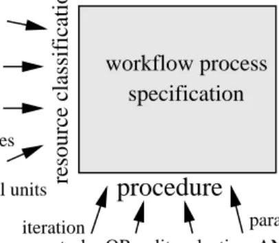
Fig. 2.The two dimensions of a workflow process specification.

Figure 2 illustrates the fact that the specification of a workflow process is composed from two elements: a procedure and a resource classification. Many WFMSs provide two workflow definition tools: one for the specification of procedures and one for the specification of resource classes. In this paper weabstract from resource classesand focus on techniques to support the construction and analysis of procedures. We also abstract from case data. In a WFMS it is possible to use case attributes when routing a case. We abstract from this information by introducing non-deterministic choices. Since case attributes are set and modified by applications and may involve human decisions, we have no other choice but to abstract from case data.

3.2 What is a workflow procedure?

The procedure specifies the set of tasks required to process cases successfully. (Syn-onyms for task are process activity, step and node.) Moreover, the procedure specifies the order in which these tasks have to be executed. (Tasks may be optional or manda-tory and are executed in parallel or sequential order.) The allocation of resources to tasks is required to decide who is going to execute a specific task for a specific case. Each resource (e.g. a secretary) is able to perform certain functions (e.g. typing a let-ter) and each task requires certain functions. A resource may be allocated to a task, if the resource provides the required functions. Recall that we concentrate on modeling

workflow procedures, i.e. we abstract from the resources required to execute these pro-cedures. To illustrate the term (workflow) procedure we will use the following example. Consider an automobile insurance company. The workflow processprocess claimtakes care of the processing of claims related to car damage. Each claim corresponds to a case to be handled by process claim. The workflow procedure that is used to handle these cases can be described as follows. There are four tasks: check insurance, con-tact garage,pay damageandsend letter. The taskscheck insuranceandcontact garage may be executed in any order to determine whether the claim is justified. If the claim is justified, the damage is paid (taskpay damage). Otherwise a ‘letter of rejection’ is sent to the claimant (tasksend letter).

3.3 Modeling a procedure

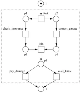
We use Petri nets for modeling and analyzing workflow procedures. Basically, a proce-dure is a partially ordered set of tasks. Therefore, it is quite easy to map a proceproce-dure onto a Petri net. Tasks are modeled by transitions and precedence relations are modeled by places. Consider for example the workflow procedureprocess claim, see Figure 3. The taskscheck insurance,contact garage,pay damageandsend letterare modeled by transitions. Since the two tasks check insuranceandcontact garagemay be exe-cuted in parallel, there are two additional transitions:forkandjoin. The placesp1,p2, p3,p4andp5are used to route a case through the procedure in a proper manner.

fork i p1 p2 contact_garage join p3 p4 p5 send_letter o pay_damage check_insurance

Fig. 3.The workflow procedureprocess claim.

Cases are processed independently, i.e. a task executed for some case cannot influence a task executed for another case. Nevertheless, the throughput time of a case may increase

if there are many other cases competing for the same resources. In this paper we abstract from resources; cases do not affect each other in any way. Therefore, it suffices to consider one case at a time. The token in placeiin Figure 3 corresponds to one case. During the processing of a case there may be several tokens referring to the same case. (If transitionforkfires, then there are two tokens, one inp1and one inp2, referring to the same claim.) The processing of the case is completed if there is a token in placeo and there are no other tokens also referring to the same case.

Petri nets which model workflow procedures have some typical properties. First of all, they always have two special placesi ando, which correspond to the beginning and termination of the processing of a case respectively. Placeiis a source place andois a sink place. Secondly, for each transitiont(placep) there should be directed path from placei too viat (p). A Petri net which satisfies these two requirements is called a Workflow net(WF-net), see Figure 1.

Definition 6 (WF-net). A Petri netPN =(P,T,F)is a WF-net (Workflow net) if and only if:

(i) PN has two special places:i ando. Placei is a source place:•i = ∅. Placeois a sink place:o• = ∅.

(ii) If we add a transitiont∗_{toPN which connects placeowithi (i.e.•t}∗ _{= {o}and}

t∗_{• = {i}), then the resulting Petri net is strongly connected.}

A WF-net has one input place (i) and one output place (o) because any case handled by the procedure represented by the WF-net is created if it enters the WFMS and is deleted once it is completely handled by the WFMS, i.e., the WF-net specifies the life-cycle of a case. The second requirement in Definition 6 (the Petri net extended witht∗ should be strongly connected), states that for each transitiont (place p) there should be directed path from placeitooviat (p). This requirement has been added to avoid ‘dangling tasks and/or conditions’, i.e. tasks and conditions which do not contribute to the processing of cases.

It is easy to verify that the Petri net shown in Figure 3 is a WF-net.

3.4 Sound procedures

The two requirements stated in Definition 6 can be verified statically, i.e. they only relate to the structure of the Petri net. There is however a third requirement which should be satisfied:

For any case, the procedure will terminate eventually, and at the moment the procedure terminates there is a token in place o and all the other places are empty.

Moreover, there should be no dead tasks, i.e., it should be possible to execute an arbi-trary task by following the appropriate route though the WF-net. These two additional constraints correspond to the so-calledsoundness property.

Definition 7 (Sound). A procedure modeled by a WF-netPN =(P,T,F)is sound if and only if:

(i) For every stateMreachable from statei, there exists a firing sequence leading from stateMto stateo. Formally:

∀M(i→∗ M)⇒(M →∗ o)

(ii) Stateo is the only state reachable from statei with at least one token in placeo. Formally:

∀M(i →∗ M ∧ M ≥o)⇒(M =o)

(iii) There are no dead transitions in(PN,i). Formally:

∀t∈T ∃M,M0 i →∗ M →t M0

Note that there is an overloading of notation: the symboliis used to denote both the place i and the state with only one token in placei (see Section 2). The soundness property relates to the dynamics of a WF-net. The first requirement in Definition 7 states that starting from the initial state (statei), it is always possible to reach the state with one token in placeo(stateo). If we assume fairness (i.e. a transition that is enabled infinitely often will fire eventually), then the first requirement implies that eventually stateois reached. The fairness assumption is reasonable in the context of workflow management; all choices are made (implicitly or explicitly) by applications, humans or external actors. Clearly, they should not introduce an infinite loop. The second requirement states that the moment a token is put in placeo, all the other places should be empty. Sometimes the termproper terminationis used to describe the first two requirements [15]. The last requirement states that there are no dead transitions (tasks) in the initial statei. For the WF-net shown in Figure 3 it is easy to see that it is sound. However, for complex workflow procedures it is far from trivial to check the soundness property.

4 Analysis of WF-nets

4.1 Introduction

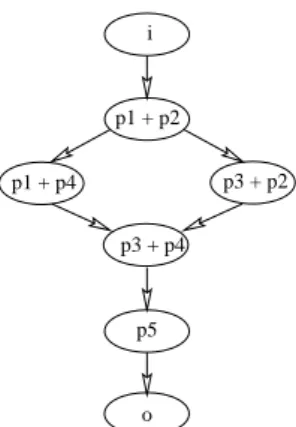
In this section, we focus on analysis techniques that can be used to verify the sound-ness property. The soundsound-ness property is a property which relates to the dynamics of a WF-net. Therefore, thecoverability graph(Peterson [21], Murata [20]) seems to be an obvious technique to check whether the WF-net is sound. Figure 4 shows the cov-erability graph which corresponds to the Petri net shown in Figure 3 (the initial state is i). There are only 7 reachable states, therefore it is easy to verify the three requirements stated in Definition 7.

In general the coverability graph can be used to decide whether a WF-net is sound. (In Section 4.2 we show that a sound WF-net is bounded. If the coverability graph has an unbounded state (an ‘ω-state’), then the WF-net is not sound. Otherwise, we can use a simple algorithm to check the three requirements stated in Definition 7.) However,

i p1 + p2 p1 + p4 p3 + p2 o p5 p3 + p4

Fig. 4.The coverability graph of the Petri net shown in Figure 3.

for complex procedures, the construction of the coverability graph may be very time consuming. The complexity of the algorithm to construct the coverability graph can be worse than primitive recursive space. Even for free-choice Petri nets the reachabil-ity problem is known to be EXPSPACE-hard (cf. Cheng, Esparza and Palsberg [9]). Therefore, any ‘brute-force approach’ to check soundness is bound to be intractable. Fortunately, the problem of deciding whether a given WF-net is sound corresponds to standard Petri-net properties. In the remainder of this section, we present a technique to decide soundness. Along the way, we encounter some interesting properties of sound WF-nets. Moreover, we will show that for most WF-net encountered in practice, the soundness property can be verified in polynomial time.

4.2 A necessary and sufficient condition for soundness

Given WF-net PN = (P,T,F), we want to decide whetherPN is sound. For this purpose we define an extended netPN =(P,T,F).PN is the Petri net that we obtain by adding an extra transitiont∗which connectsoandi. The extended Petri netPN =

(P,T,F)is defined as follows: P= P

T =T ∪ {t∗_}

F=F∪ {ho,t∗_i,ht∗_,ii}

Figure 5 illustrates the relation betweenPNandPN.

For an arbitrary WF-netPNand the corresponding extended Petri netPNwe will prove the following result:

PN is sound if and only if(PN,i)is live and bounded. First, we prove the ‘if’ direction.

PN * i t o Fig. 5.PN=(P,T∪ {t∗},F∪ {ho,t∗i,ht∗,ii}).

Proof. (PN,i)is live, i.e., for every reachable stateMthere is a firing sequence which leads to a state in whicht∗_{is enabled. Sinceois the input place oft}∗_{, we find that for} any stateMreachable from stateiit is possible to reach a state with at least one token in placeo. Consider an arbitrary reachable stateM0_{+o, i.e. a state with at least one token} in placeo. In this statet∗is enabled. Ift∗fires, then the stateM0+i is reached. Since (PN,i)is also bounded,M0should be equal to the empty state. Hence requirements (i) and (ii) hold and proper termination is guaranteed. Requirement (iii) follows directly from the fact that(PN,i)is live. Hence,PN is a sound WF-net. ut

To prove the ‘only if’ direction, we first show that the extended net is bounded.

Lemma 9. If PN is sound, then(PN,i)is bounded.

Proof. Assume thatPN is sound and(PN,i)not bounded. SincePN is not bounded there are two statesMi andMj such thati →∗ Mi,Mi →∗ Mj andMj > Mi. (See for example the proof that the coverability tree is finite in Peterson [21] (Theorem 4.1).) However, sincePN is sound we know that there is a firing sequenceσ such thatMi →σ o. Therefore, there is a stateMsuch thatMj →σ MandM >o. Hence, it is not possible thatPN is both sound and not bounded. So ifPNis sound, then(PN,i)is bounded. From the fact thatPNis sound and(PN,i)is bounded, we can deduce that(PN,i)is bounded. If transitiont∗_{inPN fires, the net returns to the initial statei. ut} Now we can prove that(PN,i)is live.

Lemma 10. If PN is sound, then(PN,i)is live.

Proof. AssumePNis sound. By Lemma 9 we know that(PN,i)is bounded. Because PN is sound we know that statei is a so-called home-marking ofPN, i.e., for every state M0 reachable from (PN,i)it is possible to return to state i. In the original net (PN,i), it is possible to fire an arbitrary transitiont(requirement (iii)). This is also the case in the modified net. Therefore,(PN,i)is live because for every stateM0reachable from(PN,i)it is possible to reach a state which enables an arbitrary transitiont. ut Theorem 11. A WF-net PN is sound if and only if(PN,i)is live and bounded. Proof. It follows directly from Lemma 8, 9 and 10. ut

Theorem 11 is an extension of the results presented in [2,24]. In [2] we restrict ourselves to free-choice WF-nets. Independently, Straub and Hurtado [24] found necessary and sufficient conditions for soundness of COPA nets. (COPA nets correspond to a subclass of free-choice Petri nets.)

Perhaps surprisingly, the verification of the soundness property boils down to check-ing whether the extended Petri net is live and bounded! This means that we can use standard Petri-net-based analysis tools to decide soundness. In Section 5 we will use Theorem 11 to prove that there is a comprehensive set of transformation rules which preserve soundness. However, first we consider an important subclass of WF-nets.

4.3 Free-choice WF-nets

Most of the WFMSs available at the moment, abstract from states between tasks, i.e., states are not represented explicitly. These WFMSs use building blocks such as the split, join, OR-split and OR-join to specify workflow procedures. The AND-split and the AND-join are used for parallel routing. The OR-AND-split and the OR-join are used for conditional routing. Because these systems abstract from states, every choice is madeinsidean OR-split building block. If we model an OR-split in terms of a Petri net, the OR-split corresponds to a number of transitions sharing the same set of input places. This means that for these WFMSs, a workflow procedure corresponds to a free-choice Petri net (see Definition 5). We have evaluated many WFMSs (e.g. the ones mentioned in Section 3.1) and just one of these systems (COSA) allows for a construction which is comparable to a non-free choice WF-net. Therefore, it makes sense to consider free-choice Petri nets. Parallelism, sequential routing, conditional routing and iteration can be modeled without violating the free-choice property (cf. Section 5). Another reason for restricting WF-nets to free-choice Petri nets is the following. If we allow non-free-choice Petri nets, then the non-free-choice between conflicting tasks may be influenced by the order in which the preceding tasks are executed. The routing of a case should be in-dependent of the order in which tasks are executed. A situation where the free-choice property is violated is often a mixture of parallelism and choice. In our opinion paral-lelism itself should be separated from the choice between a parallel and a non-parallel execution of tasks.

Free-choice Petri nets have been studied extensively and are marked by strong theoreti-cal results and efficient analysis techniques (cf. Best [8], Desel and Esparza [12,11,14], Hack [17]). As a result soundness can be determined in polynomial time for free-choice WF-nets.

Theorem 12. For a free-choice WF-net it is possible to decide soundness in polynomial time.

Proof. As a direct result of the Rank theorem ([12]), it is possible to decide liveness and boundedness in polynomial time. Therefore, the problem of checking whether a WF-net is sound can be solved in polynomial time using standard techniques. ut

Clearly, the correctness of a free-choice WF-nets can be analyzed very efficiently. Moreover, it is possible to simplify Definition 7.

Proposition 13. For free-choice WF-nets, the first two requirements in Definition 7 im-ply the third requirement.

Proof. LetPN be a free-choice WF-net satisfying the first two requirements in Defi-nition 7 ((i) and (ii)). These requirements state that the WF-net is proper terminating. It is easy to prove that the extended net(PN,i)is bounded without using the third re-quirement (see Lemma 9). Moreover, it is also easy to show thatiis a so-called home-marking ofPN. Therefore(PN,i)is deadlock-free. Since(PN,i)is a deadlock-free, bounded, strongly connected, free-choice Petri net, we deduce that(PN,i)is live (see Theorem 4.31 in Desel and Esparza [12]). Since(PN,i)is live and bounded,PN is sound (Theorem 11) and the third requirement (iii) holds. ut

Most of the workflow procedures we have seen in practice obey the free-choice prop-erty. This is a direct result of the fact that most of the workflow systems abstract from the explicit modeling of states. However, a Petri-net-based WFMS such as COSA (Software-Ley, Pullheim, Germany) allows for the construction of non-free-choice WF-nets. Fortunately, for non-free-choice WF-nets we can check a sufficient condition for soundness in polynomial time.

In the following theorem we assume that the reader is familiar with some advanced notions: rank, siphon and cluster. A cluster is a minimal setC of nodes satisfying the following conditions. If the set contains a places, thens• ⊆ C. If the set contains a placet, then•t ⊆C. For more information on these advanced topics, we refer to [12] and [20].

Theorem 14. A WF-net PN is sound if the rank of PN is equal to the number of clusters minus 1 and every proper siphon contains at least one token.

Proof. PN is strongly connected. Therefore we can apply Theorem 10.17 in [12]. This theorem states that a weakly connected Petri net with at least one place and one transi-tion, a rank equal to the number of clusters minus 1 (i.e.Rank(PN)= |CN| −1) and a token in every proper siphon, is live and bounded. By applying Theorem 11 we deduce

thatPN is sound. ut

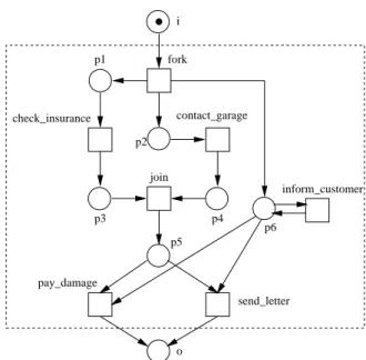
The conditions stated in Theorem 14 are sufficient for soundness and can be checked in polynomial time. Figure 6 shows a WF-net which is not free-choice. The two transitions pay damageandsend letterare in conflict with the new transitioninform customerbut the sets of input places differ. The rank of the extended WF-net is 5, the number of clusters is 6 and every proper siphon contains at least one token. Therefore, we can use Theorem 14 to prove that the WF-net is sound (in polynomial time).

Unfortunately, there are sound WF-nets which do not satisfy the conditions stated in Theorem 14. However, we can extend the class of free-choice WF-nets such that these conditions are necessary and sufficient for soundness. A Petri net that belongs to this class is called analmost free-choiceWF-net.

Definition 15 (Almost free-choice). A Petri net is analmost free-choice Petri netiff, for every two transitionst1andt2either

fork i p1 join p3 p4 p5 o pay_damage check_insurance contact_garage send_letter inform_customer p2 p6

Fig. 6.The modified procedureprocess claim.

- (•t1 ∩ •t2)= ∅, or

- •t1 = •t2, or

- •t1 = t1• and •t1 ⊆ •t2, or

- •t2 = t2• and •t2 ⊆ •t1.

An almost free-choice Petri net is a free-choice Petri net extended with zero or more transitions which can not change the state of the net and preserve (non)liveness of the net. The additional transitions correspond to inquiry tasks, i.e. tasks which do not con-tribute to the processing of a case. These tasks are executed if someone requires in-formation about a particular case. The WF-net in Figure 6 is almost free-choice; in-form customercorresponds to a so-called inquiry task.

Theorem 16. For an almost free-choice WF-net it is possible to decide soundness in polynomial time.

Proof. An almost free-choice WF-net can be transformed into a free-choice WF-net without changing liveness and boundedness properties. This can be done by simply removing the inquiry transitions. An inquiry transition is a transitiont1 such that (1)

•t1 = t1• and (2) there is another transitiont2 such that •t1 ⊆ •t2. Removing

t1 does not change boundedness, becauset1cannot change the state. Liveness is also

not affected becauset1cannot change the state andt1is live ift2is live. By removing

all inquiry transitions we obtain a free-choice WF-net. Then we can apply the Rank

theorem to decide soundness. ut

These results show that for a fairly large class of WF-nets we can decide soundness very efficiently. We have been involved in a number of workflow projects (Dutch Customs

department, Dutch Justice department and a number of banks and insurance compa-nies). In these projects we hardly ever experienced the need for WF-nets which are not almost free-choice.

5 Transformation rules

One of the major benefits of a WFMS is the ability to change business processes very easily, i.e., without a complete redesign of the information system. Moreover, work-flow mangement software is an essential enabler for management philosophies such as Business Process Reengineering (BPR) and Continuous Process Improvement (CPI). BPR and CPI are also a stimulus for the modification of business processes. As a result, the procedures supported by the WFMS are subject to frequent changes. These changes may introduce errors. In this paper we have shown that it is possible to check the sound-ness of a procedure very efficiently. However, we can use an alternative approach to make sure that the procedure remains sound. This approach is based onsoundness pre-serving transformation rules.

In our opinion there are eight basic transformation rules (T1a,T1b,T2a,T2b,T3a, T3b,T4a andT4b) which can be used to modify a sound workflow procedure. These transformation rules are shown in Figures 7, 8, 9 and 10 and elucidated in the sequel. The transformation rules correspond to the basic routing constructs identified by the Workflow Management Coalition ([26]). These rules should not be confused with the reduction rules presented in Petri-net literature (cf. Berthelot [7], Desel [10], Desel and Esparza [12] and Kovalyov [19]). The transformation rules presented in this section are not used for analysis purposes; they are used for the modification of WF-nets.

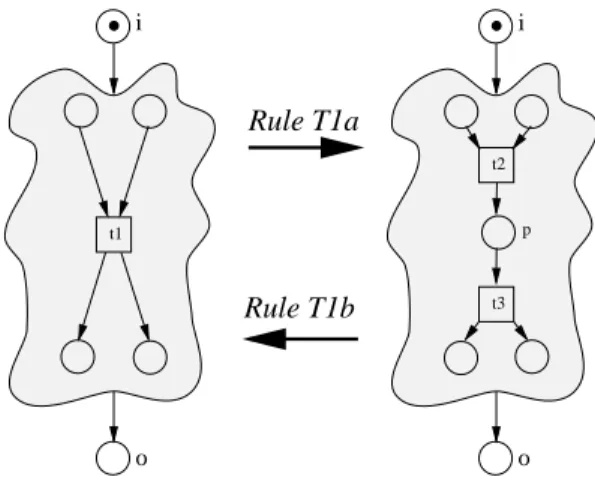
T1a Taskt1 is replaced by two consecutive taskst2 andt3. This transformation rule corresponds to thedivisionof a task: a complex task is divided into two tasks which are less complicated. (See Figure 7.)

i o t1 i o t2 t3 p Rule T1a Rule T1b

T1b Two consecutive taskst2 andt3 are replaced by one taskt1. This transformation rule is the opposite ofT1aand corresponds to theaggregationof tasks. Two tasks are combined into one task. (See Figure 7.)

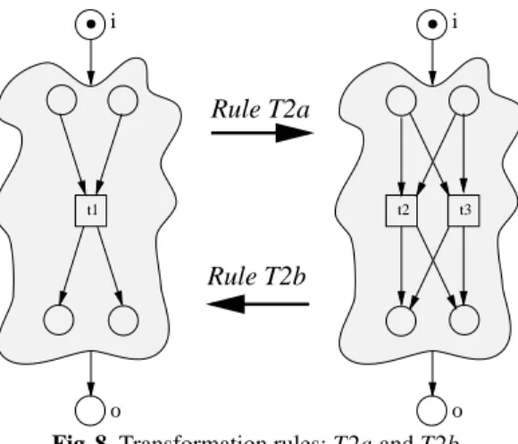
T2a Taskt1 is replaced by two conditional taskst2 andt3. This transformation rule corresponds to thespecializationof a task (e.g.handle order) into two more spe-cialized tasks (e.g.handle small orderandhandle large order).

(See Figure 8.) i o t1 i o Rule T2a Rule T2b t2 t3

Fig. 8.Transformation rules:T2aandT2b.

T2b Two conditional taskst2 andt3 are replaced by one taskt1. This transformation rule is the opposite ofT2a and corresponds to the generalization of tasks. Two rather specific tasks are replaced by one more generic task. (See Figure 8.) T3a Taskt1 is replaced by two parallel taskst2 andt3. (See Figure 9.) The effect of the

execution oft2 andt3 is identical to the effect of the execution oft1. The transitions c1 andc2 represent control activities to fork and join two parallel threads.

T3b The opposite of transformation ruleT3a: two parallel taskst2 andt3 are replaced by one taskt1. (See Figure 9.)

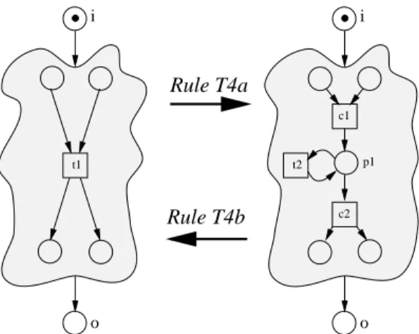
T4a Taskt1 is replaced by an iteration of taskt2. (See Figure 10.) The execution of taskt1 (e.g.type letter) corresponds to zero or more executions of task t2 (e.g. type sentence). The transitionsc1 andc2 represent control activities that mark the begin and end of a sequence of ‘t2-tasks’. Typical examples of situations where iteration is required are quality control and communication.

T4b The opposite of transformation ruleT4a: the iteration oft2 is replaced by taskt1. (See Figure 10.)

Formalization of these transformation rules is straightforward. To illustrate this we de-fineT1a. (See Figure 7.)

Definition 17 (T1a). LetPN =(P,T,F)be WF-net. This net can be transformed by rule T1a into a netPN0 _=(P0_,T0_,F0_{)iff there existt1∈ T,t2,t3 ∈T}0_{and p ∈ P}0 such that P0 _{= P ∪ {p}, p 6∈ P,T}0 _{= (T \ {t1})∪ {t2,t3},{t2,t3} ∩T = ∅and}

i o t1 i o t3 t2 c2 c1 p2 p1 p3 p4 Rule T3a Rule T3b

Fig. 9.Transformation rules:T3aandT3b.

i o t1 i o c2 c1 Rule T4a Rule T4b p1 t2

F0_{= {hx,yi ∈F|(x6=t1)∧(y6=t1)} ∪ {hx,t2i ∈P×T | hx,t1i ∈F} ∪ {ht3,yi ∈}

T ×P| ht1,yi ∈F} ∪ {ht2,pi,hp,t3i}.

It is easy to see that if we take a sound WF-net and we apply one of these transformation rules, then the resulting Petri net is still a WF-net. Moreover, the resulting WF-net is also sound.

Theorem 18. The transformation rules T1a, T1b, T2a, T2b, T3a, T3b, T4a and T4b preserve soundness, i.e. if a WF-net is sound, then the WF-net transformed by one of these rules is also sound.

Proof. LetPNbe a sound WF-net. LetPN0be a net which is obtained by applying one of the transformation rules onPN. We have to prove thatPN0is a sound WF-net. It is easy to see thatPN0is a WF-net. There is still one input and one output place and the PN0_{is strongly connected. (PN}0_{is the Petri netPN}0_{with an extra transitiont}∗_which connects placeo and place i.) By Theorem 11 we know that, to prove soundness, it suffices to show(PN0_{,i)is live and bounded.(PN,i)is live and bounded. Therefore,} we have to prove that each of the rules preserves liveness and boundedness. Because it is obvious that the rules preserve liveness and boundedness, we do not give a detailed proof. It is for example possible to prove this by using the 6 liveness and boundedness

preserving operations described in Murata [20]. ut

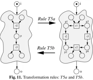
The eight transformation rules shown in figures 7, 8, 9 and 10 preserve soundness. We can use these basic transformation rules to construct more complex transformation rules. Figure 11 shows two of these rules:T5aandT5b.

T5a Two consecutive tasks are replaced by two parallel tasks. T5b Two parallel tasks are replaced by two consecutive tasks.

i o i o t3 t2 c2 c1 p2 p1 p3 p4 t2 t3 p Rule T5a Rule T5b

Fig. 11.Transformation rules:T5aandT5b.

The application of transformation ruleT5a corresponds to the application ofT1b fol-lowed by the application ofT3a. Transformation ruleT5bis a combination ofT3band

T1a. Therefore, soundness is also preserved by the transformation rulesT5aandT5b. We use the term ‘sound transformation rule’ to refer to a transformation rules which preserves soundness.

The WF-net which comprises only one taskt is sound. We can use this net as a start-ing point for a sequence of sound transformations. By Theorem 18 we know that the resulting WF-net is sound.

Corollary 19. If the Petri net PN = ({i,o},{t},{hi,ti,ht,oi})is transformed into a Petri net PN0 _{by applying a sequence of sound transformation rules (e.g. T1a, T1b,}

T2a, T2b, T3a, T3b, T4a, T4b, T5a and T5b), then PN0_{is sound.}

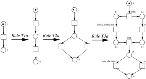
Consider for example the WF-net shown in Figure 3. We can construct this net by applying the transformation rulesT1a,T2aandT3a, see Figure 12.

fork i p1 contact_garage join p3 p5 send_letter pay_damage check_insurance p2 p4 o i o

Rule T1a Rule T2a

i

o o

Rule T3a

i

Fig. 12.Construction of the WF-net shown in Figure 3.

Note that the converse of Corollary 19 is not true. There are sound WF-nets which cannot be constructed by the transformation rules defined in this section. Consider for example the WF-net shown in Figure 6; this net is sound but cannot be constructed by using the transformation rules. Nevertheless, the rules correspond to the basic routing primitives present in most WFMSs.

6 Related work

Many researchers have inversigated properties similar to the soundness property. Straub and Hurtado [24] have analyzed a similar property for COPA nets. The soundness prop-erty is also closely related to Valette’s concept of a well-formed block [25] and Gostel-low’s concept of proper termination [15]. There is also a relation between reversibility (the possibility to return to the initial state, i.e., the initial state is a home-marking)

and soundness. The results presented in this paper are marked by the fact that they are valid for any WF-net. Moreover, we have showed that for an important subclass (almost free-choice) the soundness property can be verified in polynomial time.

The use of Petri nets in the workflow domain is increasing. At the moment several Petri-net-based workflow tools are available. COSA (Software-Ley) is a Petri-net-based workflow management system. COSA is one of the leading workflow products in Eu-rope. LEU (LION/Vebacom) is a WFMS based on FUNSOFT nets ([16]). INCOME (Promatis) and StructWare/BusinessSpecs (IvyTeam) are both Petri-net-based BPR tools which can be used to configure a WFMS. INCOME interfaces with Designer/2000 (Or-acle), Plexus (BacTec) and CSE/Workflow (CSE systems). StructWare/BusinessSpecs interfaces with Staffware (Staffware), one of the worlds leading WFMSs. These tools show that workflow managemant is becoming an important application domain for Petri nets. However, these Petri-net-based workflow tools do not support advanced analysis techniques. Therefore, we have developedWOFLAN(WOrkFLow ANalyser). WOFLAN is a Petri-net-based analysis tool for the verfication of workflows. Amongst others it supports the analysis techniques described in this paper.

7 Conclusion

In this paper we have presented a class of Petri nets, the so-called WF-nets, suitable for the representation, validation and verification of workflow procedures. One of the mer-its of this class is that we can verify the soundness property using standard techniques. Moreover, we have identified an important class of WF-nets that can be verified in poly-nomial time. Even though sound WF-nets have some nice properties from a theoretical point of view, they are powerful enough to model any workflow procedure. Moreover, we have shown that the plausible transformation rules encountered in practice preserve soundness.

In this paper we focused on the workflow procedures supported by a WFMS. To com-pletely specify a workflow process we also have to specify the management of re-sources: given a task that needs to be executed for a specific case we have to specify the resource (person or machine) that is going to process the task (cf. Van der Aalst and Van Hee [5]). A direction for further research is to incorporate this dimension. We hope to find a necessary and sufficient condition for soundness given a WF-net extended with some mechanism to allocate resources to tasks.

References

1. W.M.P. van der Aalst. Putting Petri nets to work in industry. Computers in Industry, 25(1):45–54, 1994.

2. W.M.P. van der Aalst. A class of Petri net for modeling and analyzing business processes. Computing Science Reports 95/26, Eindhoven University of Technology, Eindhoven, 1995. 3. W.M.P. van der Aalst. Petri-net-based Workflow Management Software. In A. Sheth,

edi-tor,Proceedings of the NFS Workshop on Workflow and Process Automation in Information Systems, pages 114–118, Athens, Georgia, May 1996.

4. W.M.P. van der Aalst. Three Good reasons for Using a Petri-net-based Workflow Man-agement System. In S. Navathe and T. Wakayama, editors,Proceedings of the International Working Conference on Information and Process Integration in Enterprises (IPIC’96), pages 179–201, Camebridge, Massachusetts, Nov 1996.

5. W.M.P. van der Aalst and K.M. van Hee. Business Process Redesign: A Petri-net-based approach.Computers in Industry, 29(1-2):15–26, 1996.

6. W.M.P. van der Aalst and K.M. van Hee. Workflow Management: Modellen, Methoden en Systemen (in Dutch). Academic Service, Schoonhoven, 1997.

7. G. Berthelot. Transformations and decompositions of nets. In W. Brauer, W. Reisig, and G. Rozenberg, editors, Advances in Petri Nets 1986 Part I: Petri Nets, central mod-els and their properties, volume 254 ofLecture Notes in Computer Science, pages 360–376. Springer-Verlag, Berlin, 1987.

8. E. Best. Structure theory of Petri nets: the free choice hiatus. In W. Brauer, W. Reisig, and G. Rozenberg, editors,Advances in Petri Nets 1986 Part I: Petri Nets, central models and their properties, volume 254 of Lecture Notes in Computer Science, pages 168–206. Springer-Verlag, Berlin, 1987.

9. A. Cheng, J. Esparza, and J. Palsberg. Complexity results for 1-safe nets. In R.K. Shyama-sundar, editor,Foundations of software technology and theoretical computer science, volume 761 ofLecture Notes in Computer Science, pages 326–337. Springer-Verlag, Berlin, 1993. 10. J. Desel. Reduction and design of well-behaved concurrent systems. In J.C.M. Baeten

and J.W. Klop, editors, Proceedings of CONCUR 1990, volume 458 ofLecture Notes in Computer Science, pages 166–181. Springer-Verlag, Berlin, 1990.

11. J. Desel. A proof of the Rank theorem for extended free-choice nets. In K. Jensen, edi-tor,Application and Theory of Petri Nets 1992, volume 616 ofLecture Notes in Computer Science, pages 134–153. Springer-Verlag, Berlin, 1992.

12. J. Desel and J. Esparza.Free choice Petri nets, volume 40 ofCambridge tracts in theoretical computer science. Cambridge University Press, Cambridge, 1995.

13. C.A. Ellis and G.J. Nutt. Modelling and Enactment of Workflow Systems. In M. Ajmone Marsan, editor,Application and Theory of Petri Nets 1993, volume 691 ofLecture Notes in Computer Science, pages 1–16. Springer-Verlag, Berlin, 1993.

14. J. Esparza. Synthesis rules for Petri nets, and how they can lead to new results. In J.C.M. Baeten and J.W. Klop, editors,Proceedings of CONCUR 1990, volume 458 ofLecture Notes in Computer Science, pages 182–198. Springer-Verlag, Berlin, 1990.

15. K. Gostellow, V. Cerf, G. Estrin, and S. Volansky. Proper Termination of Flow-of-control in Programs Involving Concurrent Processes. ACM Sigplan, 7(11):15–27, 1972.

16. V. Gruhn. Validation and Verification of Software Process Models. In A. Endres and H. We-ber, editors,Software Development Environments and CASE Technology, volume 509 of Lec-ture Notes in Computer Science, pages 271–286. Springer-Verlag, Berlin, 1991.

17. M.H.T. Hack. Analysis production schemata by Petri nets. Master’s thesis, Massachusetts Institute of Technology, Cambridge, Mass., 1972.

18. T.M. Koulopoulos.The Workflow Imperative. Van Nostrand Reinhold, New York, 1995. 19. A.V. Kovalyov. On complete reducability of some classes of Petri nets. InProceedings of

the 11th International Conference on Applications and Theory of Petri Nets, pages 352–366, Paris, June 1990.

20. T. Murata. Petri Nets: Properties, Analysis and Applications. Proceedings of the IEEE, 77(4):541–580, April 1989.

21. J.L. Peterson.Petri net theory and the modeling of systems. Prentice-Hall, Englewood Cliffs, 1981.

22. C.A. Petri. Kommunikation mit Automaten. PhD thesis, Institut f¨ur instrumentelle Mathe-matik, Bonn, 1962.

23. T. Sch¨al. Workflow Management for Process Organisations, volume 1096 ofLecture Notes in Computer Science. Springer-Verlag, Berlin, 1996.

24. P.A. Straub and C. Hurtado. The Simple Control Property of Business Process Models. In XV International Conference of the Chilean Computer Science Society, 1995.

25. R. Valette. Analysis of Petri Nets by Stepwise Refinements.Journal of Computer and System Sciences, 18:35–46, 1979.

26. WFMC. Workflow Management Coalition Terminology and Glossary (WFMC-TC-1011). Technical report, Workflow Management Coalition, Brussels, 1996.