Object Tracking Based on Online Classification Boosted by Discriminative Features

Object Tracking Based on Online Classification Boosted by

Discriminative Features

Yehong Chen

1

and Pil Seong Park

2 1

Qilu University of Technology, China

2

University of Suwon, Korea

[email protected], [email protected]

Abstract

We propose a robust object tracking algorithm under “tracking by detection” framework. A sparse random Gaussian-distributed measurement matrix is used to build an object appearance model in the compressed domain, and detection is done by our semi-supervised learning process. Our method trains a group of weaker classifiers corresponding to every feature, and linearly combines them using the weights computed by its discriminative power to build a strong classification function, which detects a target from background. Kalman filtering is also adopted to smoothen the tracking results. Experiments show the proposed

classification improves performance in tracking without drift.

Keywords: Object tracking, Sparse random measurement matrix, Naive Bayes classifier, Discriminative power , Feature selection, Kalman filter

1. Introduction

Object tracking is an important task within the field of computer vision, and its application area is broad. It is a challenging problem due to numerous factors like appearance changes, viewpoints of moving objects, and a cluttered background under different illumination conditions. Significant progress has been made during these years. Tracking and associated problems of feature selection, object representation, dynamic shape, and motion estimation became very active research areas and new solutions are being proposed [14].

In what is called "tracking by detection", an object is often represented by a vector in a feature space, and a tracking task is formulated as a binary c lassification problem so that each image in a video sequence is classified into either a target or a background [12]. This kind of tracking algorithms consist of a few main steps: feature extraction, feature selection, classifier training, and detection in every frame. In reality, the representation of an object is in a very high dimensional space of complete features, causing the curse of dimensionality. There are some methods involved in such a problem, and sparse representation obtained by L1 norm minimization [3] is one such example. When building an object’s appearance model, feature extraction and feature selection are two main ways directly related to dimensionality reduction.

Recently the compressive sensing method has been successfully introduced in object tracking [15], making use of sparse representation of a target. We call their algorithm RCT for short. Even though RCT is an outstanding pioneering work that combines various state-of-the-art techniques in a concise manner, we found that it can be further

2

improved by adopting an explicit feature selection process and an inter -frame prediction mechanism for robust object tracking.

In recent years, feature selection has been attractive, and a lot of work has been done [4, 7, 10, 11, 13]. The goal of feature selection is to pick a good subset of features from some large set of candidate features [6]. Feature selection plays an important role in performance of classification. Our main idea is to formulate feature’s discriminative power from training data, and utilizing it to weigh extracted features. These feature weights can be used to boost weaker classifiers (corresponding to individual features) to a strong classification, which replaces the classifier in RCT. For inter-frame prediction, we adopt the Kalman filter, which also allows single-frame measurement of hidden states both for the position of tracking objects and the feature weights.

This paper is organized as follows: In Section 2, we introduce some related works. In Section 3, we introduce the fundamental principles from which our method is deduced. In Section 4, experimental results are presented with discussion and analysis on how and why our method works well, followed by conclusion and future works.

2. Related Works

2.1. RCT

The real-time compressive tracking (RCT) method by Zhang et al., [15] is a

state-of-the-art algorithm, in terms of efficiency, accuracy and robustness. The following is a brief summary about RCT [1, 2, 8, 15].

RCT is a tracking algorithm with an appearance model based on the features extracted from a multi-scale image feature space with a data-independent basis. Its appearance model employs non-adaptive random projections that preserve the structure of the image feature space of objects. A tracking task is formulated as a binary classification via a naive Bayes classifier with online update in a compressed domain.

The whole tracking process consists of two stages: learning and detection. A target is manually labeled only at the beginning in a given video, and training data is associated automatically with the previous tracking result afterwards. In the learning stage, given the captured target by the previous tracking result, the algorithm crops training samples (both the target and the background), around the target’s position in some predefined region, which are then used for learning/updating the classifier. In the next frame, the detector samples patches as input to the classifier to look for the target. Finally the algorithm identifies the position of the sample patch with maximum posteriori as the

position of the object. Then the entire two-stage tracking process is repeated.

2.1.1. Feature extraction and dimensionality reduction in RCT

In video tracking, each image patch can be represented by a vector

x



m, and let

m

X be a feature space. A feature dictionary is a basis of the feature space X. The

number

m

of features in the dictionary can be huge, and any object can be represented by a

linear combination of

n

feature basis vectors, where n m.

RCT uses the feature extraction approach based on compressive sensing by introducing a

sparse random Gaussian measurement matrix n m

R  to project a high-dimensional image

vector x m onto a lower dimensional one v n _by

v



R

x

(1) where the ( , )i j -th component of R is given by

with probability 1/2s with probability 1 - 1/s, with probability 1/2s

RCT uses s=m/4, hence R is very sparse, requiring very low computational complexity

[1, 15]. Since the nonzero entries of R are either 1 or -1, the compressive features compute the

relative intensity difference in a way similar to generalized Haar-like features, which is a

linear combination of randomly generated rectangles [2, 6, 15]. As an illustration, see Figure

1. Every group of rectangles in the same color corresponds to a random Haar-like feature. The

figure on the right is a general template for feature extraction.

Figure 1. Features within a sample frame. The movie is from [16]

2.1.2. The naive Bayes classifier in RCT

For tracking by detection, we need a trained classifier that can distinguish two classes of

samples, i.e., target samples and background samples in the feature space. Let

{( ,

x y

_{i i}

) :

i



1, 2,... ,

s y

_{n i}



{0,1}}

be the training data, where each

x

_i is a training sample in

the set X m, and v_i n is its low-dimensional representation.

s

_n is the number of

training samples, and

y

_i is a class label, i.e., 0 for negative and 1 for positive samples.

RCT uses a naive Bayes classifier. Samples satisfy the following conditional probability 1 ( | 1) n ( |_i 1) ( 1) i p v y 



_ p v y p y , ( | 0) n₁ (_i| 0) ( 0) i p v y 



_ p v y p y .

If p v y( |  1) p v y( | 0), v will be labeled as positive, and negative otherwise. A naive Bayes classifier uses a log ratio to represent the classifier function. RCT selects the sample with the largest F(v) as the target measurement, where

(2)

2.2. Kalman filter

The Kalman filter is a recursive estimator that uses a series of measurements observed over time, containing noise and other inaccuracies, and produces estimates of unknown variables that tend to be more precise than those based on a single measurement alone. More formally, the Kalman filter operates recursively on streams of noisy input data to produce a statistically optimal estimate of the underlying system state.

Object tracking can be thought of as a hidden Markov chain problem. Detection by classification focuses on the current frame only, and it does not reflect the translation of the object between two consecutive frames. To deal with linking between two

1 0 1 ij r s    _    1 1 1 ( | 1) ( 1) _{( | 1)} ( ) log log ( | 0) ( | 0) ( 0) n n i i i n i i i i p v y p y _{p v y} F v p v y p v y p y     _{ }  _{ }     _{ } _{ } _        



_



consecutive frames, we adopt Kalman filtering. Figure 2 shows the role of the Kalman filter in tracking [5, 7].

Figure 2. Kalman filtering in tracking by detection

3. Proposed Algorithm

In visual object tracking, the most desirable property of a feature is its uniqueness so that the object is easily distinguishable in the feature space [6, 14]. Furthermore, the features that best discriminate between the target and the background are desirable. A traditional way is choosing features manually, depending on the application domain. In machine learning and pattern recognition communities, a wide range of automatic

feature selection algorithms have been investigated,for example, AdaBoost is a popular

algorithm widely used in machine learning community [11]. However, most of these methods need offline training, huge training data, a long training period, and all the information known in advance. For object tracking, online selection of discriminative features is more suitable due to the change in object appearance frame by frame.

Through the analysis of the source code of RCT obtained from [16], we found that it lacks an explicit feature selection process according to the characteristics of special objects. Its feature extraction process uses an off-line calculated random Gaussian measurement matrix, keeping the same feature templates throughout the tracking task. However we formulate feature’s discriminative power from training data, and use it to weigh both the relevant and

irrelevant features. These feature weights are then used to boost weaker classifiers (i.e., naive

Bayes classifiers) to a strong classification, which can replace the classifier in RCT.

We train our classification model in two steps: first, learn a group of weaker classifiers f

corresponding to every feature (assuming vi has an independent distribution with each other)

respectively. Then assign a weight vector to weaker classifiers to boost to a strong classification. The job can be done by any of feature selection methods, but there is some trade-off. We do not use one of the off-the-shelf feature selection modules, but formulate feature’s discriminative power from training data to maintain high efficiency and at the same time to improve tracking accuracy. This method may be thought of as a simple replacement of the Fisher discriminant which is used to evaluate feature’s discriminative power in classifier training, but our method is simpler and easy to realize.

3.1. Weak classifiers

RCT treats all extracted features equally important without considering the explicit structure of the target. However not all features are of equal importance.

In our method, unlike (2), we introduce max so that f v( )_i 0.

( ) max{0,log ( | 1) } ( | 0) i i i p v y f v p v y     _ _    (3)

f can be used as a weaker classifier corresponding to every feature. These will be combined to form a strong classification, and some irrelevant features can be removed by setting their weights to 0.

For a random sample in images, we assume the uniform prior, p y(  1) p y( 0). The

random projections of high dimensional vectors are known to be almost always Gaussian distributed. Thus, the conditional distributions p v(_i|y1) and p v(_i|y0) in f v( )_i are

assumed to be Gaussian distributed, with four parameters (µi

1_,σ i 1 , µi 0 , σi 0 ), where µi 1 and σi 1

are the mean and the standard deviation of the positive sample set X1 in the i-th feature, and

µi 0

and σi 0

are the mean and the standard deviation of the negative sample set X0 in the i-th

feature, i.e.,

(i| 1)

p v y ~ N(µi1,σi1 ), and p v( i|y0) ~ N(µi0,σi0 ) .

( )_i

f v is learned and updated online, according to the training sample sets X1 and X0.

3.2. Strong classification boosted by discriminative power of features

After learning a group of weaker classifiers f (vi) corresponding to each feature, we need to

get a weight vector n

W to build a strong classification as a linear combination of them.

We want to use a simple and direct way to find W=(W1,…,Wn) and online boost weaker

classifiers to a strong classification.

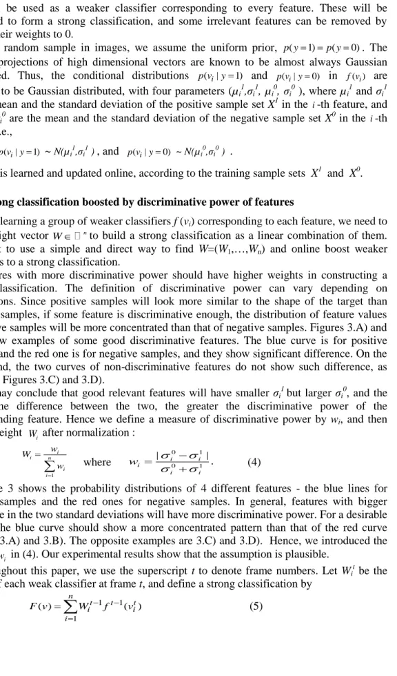
Features with more discriminative power should have higher weights in constructing a strong classification. The definition of discriminative power can vary depending on applications. Since positive samples will look more similar to the shape of the target than negative samples, if some feature is discriminative enough, the distribution of feature values of positive samples will be more concentrated than that of negative samples. Figures 3.A) and 3.B) show examples of some good discriminative features. The blue curve is for positive samples and the red one is for negative samples, and they show significant difference. On the other hand, the two curves of non-discriminative features do not show such difference, as shown in Figures 3.C) and 3.D).

We may conclude that good relevant features will have smaller σi

1

but larger σi 0

, and the bigger the difference between the two, the greater the discriminative power of the

corresponding feature. Hence we define a measure of discriminative power by wi, and then

form a weight W_i after normalization :

where (4)

Figure 3 shows the probability distributions of 4 different features - the blue lines for positive samples and the red ones for negative samples. In general, features with bigger difference in the two standard deviations will have more discriminative power. For a desirable feature, the blue curve should show a more concentrated pattern than that of the red curve (Figures 3.A) and 3.B). The opposite examples are 3.C) and 3.D). Hence, we introduced the

measurew_i in (4). Our experimental results show that the assumption is plausible.

Throughout this paper, we use the superscript t to denote frame numbers. Let Wi

t

be the

weight of each weak classifier at frame t, and define a strong classification by

1 1 1 ( ) ( ) n t t t i i i F v W  f  v  



(5) 1 i i n i i w W w  



0 1 0 1 | | . i i i i i w       

This classification model is online refreshed, and is beneficial to identify the main

characteristics under noisy condition. In (5), weaker classifiers f are boosted by the weight

vector Wi t

to a strong classification F.

A) B) C) D)

Figure 3. The distribution of four feature values. The first two have more discriminative power than the other two

Our algorithm may look similar to general boosting algorithms, but there is a significant difference. Most boosting algorithms have iteratively learning weak classifiers with respect to data distribution and add them to form a strong classifier. When weak classifiers are added, they are typically weighted in some way that is usually related to weak learner’s accuracy. The iteration is generally expected to converge finally, or it stops at a preset iteration upper bound. As a consequence, the number of weak classifiers is not certain.

However, in our method, weak classifiers are weighted in some way that is related to feature’s discriminative power rather than their accuracy. In addition, there is no iteration. The advantage of our method is that it is simple and quick enough so that it can be used for online training.

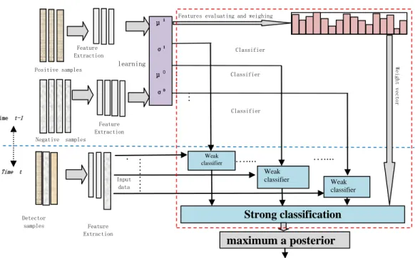
Figure 4 is the schematic diagram of our strong classification. The red dotted box shows the difference from that of RCT.

Figure 4. A schematic diagram of our strong classification

Feature Extraction

Features evaluating and weighing Positive samples Negative samples Time t-1 Time t …… … . . Input data ………… … W eight vector ….... ….... Feature Extraction Weak classifier Weak classifier Detector samples Feature Extraction Weak classifier Strong classification learning Classifier parameters maximum a posterior detection result Classifier parameters Classifier parameters μ1 σ1 μ0 σ0

3.3. Tracking results

At the t-th frame, let the previous sample response be zt-1=(x,y,w,h), where xt-1=(x,y) is its

coordinate, and w and h are its width and height, respectively. Let Wt-1 be the weight in the

previous frame. Let dn be the number of detector samples, and Vt{V₁t,...,V_jt:j1,...,d_n} be the

representation of current detector samples which are centered at the point within a certain searching radius from the prior position. The next sample response will be taken as the one

with maximal value of F:

arg max

j

J F(Vjt), j=1,2,…,dn. (6)

In detection stage, the algorithm samples patches within a predefined search region. Then the classifier looks for the target by looking for the sample patch with maximum posteriori. 3.4. Smoothing by Kalman filter

Object tracking can be thought of as a hidden Markov chain problem. Detection by classification in general only focuses on the current frame, and it does not reflect the translation between two consecutive frames. So far, we did not consider the movement of a target object. However to deal with linking between frames, we now adopt a Kalman filter. In our tracking application, hidden states are the object’s position and feature’s weight, and the Kalman filter will calculate the estimated states.

Our Kalman filter built on a simple motion model is as follows:

t

and tare noises which obey Gaussian distribution. Wt is the weight vector and xt is

the object’s actual position. We initialize the weight of each feature bin by setting Wi 0

=1/n

and  Wi

0

=0 for all i. x0 is manually initialized in the first frame and setΔx0 =0. xK and WK

are the measurements obtained from the detection and learned classifier. Since the position update and the weight update can be done independently, we use two different Kalman filters,

say, KalmanP for position and KalmanF for weight, respectively.

3.5. Our algorithm

Summing up, the flow of our full algorithm is shown in Figure 5. The detail of the algorithm is shown in Algorithms 1, 2, and 3 below.

0 0 0 0 0 0 t t t n n t K t t m m K t W I W W I           _{ }       _{  }     _{ }  _    x x x 1 1 1 1 0 0 0 0 0 , 0 0 0 0 0 t t n n n n t t n n t t t m m m m t t m m I I W W I W W I I I                _   _   _  _{ }           _  _{ }_      x x x x

Figure 5. Overall flow of our algorithm

Algorithm 1. Online learning and update

Input: t-th video frame and the previous tracked location xt

Output: weaker classifier parameter vector pit, weight vector Wt

1. Sample two sets of image patches,

i.e., a positive sample set X1={xi | ||xi – x t

|| ≤ α, i=1,…,r} and a negative sample set X0={xj | β ≤ || xj - x

t

|| ≤ γ, i=1,…,r } where i and j are indices of patches,

α, β, γ (α< β< γ) are appropriately chosen parameters,

and r is the number of image patches.

2. Extract features V with low dimensionality using (1).

3. Learn the parameters pi

t =(µi 1_,σ i 1 , µi 0_,σ i 0

) for each weaker classifier f (vi).

4. Learn the weight vector Wk

t

by (4).

5. To correct Wk

t

,

use the Kalman filter to obtain Wt = KalmanF(Wk

t

,ΔWt ) where Δ Wt =Wk t_–

Wt-1. Algorithm 2. Detection

Input: (t+1)-th frame, weaker classifier parameters pi t

, and boosted weight vector Wt

Output :xt +1

1. Sample a set of image patches Dδ ={ xi | ||xi-x t _||<δ}

where xt is the tracking location at the t-th frame,

and extract features V with low dimensionality.

2. Use the boosted classification F to each sample vector V

and find the tracking location xt+1 with the maximal classification response by (6).

3. Use the Kalman filter to get corrective position

by xt+1=KalmanP(xt+1, x) where x = xt+1- xt. Algorithm 3. Tracking by detection

Input: initial target position x0 and Δx0 =0. Output: tracking results

1. Initialize the Kalman filter with Wi

0

=1/n and  Wi 0

=0 for all i.

2.1)Execute Algorithm 1 (Online Learning and update). 2.2) Execute Algorithm 2 (Detection).

In our full algorithm, we apply the Kalman filter both to the position of the object and to the weight. However, to estimate the effect of the Kalman filter, we devise two variants of our full algorithm, depending on where we apply the Kalman filter. They are summerized as follows:

SigKK : Our full algorithm. Use both KalmanP and KalmanF. (=SigKPF)

SigKP : A variant using KalmanP only.

SigKF : A variant using KalmanF only

4. Experiments and Results

We compare the result of RCT with those of our full algorithm (sigKK) and its variants (SigKP and SigKF) using the public dataset ‘David indoor’ from [16]. We used the same

parameters (i.e., α=4, β=5, γ=20 in Algorithms 1 and 2). Other parameters like δ or the width

and height of the patch sampled are decided by manually marking the object at the beginning of the run.) as that the authors used in [15] except for the number of features, which we increased from 50 to 100. We manually marked the exact position of the object and drew a bounding box to compare with the results by the above methods.

Figure 6 shows the comparison. The white boxes are the bounding boxes around the actual positions, while the blue ones are by RCT, the green ones by sigKP, and the red ones by sigKK. As we can see in Figure 6, red ones are the closest to white boxes while the blue ones by RCT are the farthest.

Red - sigKK White - actual position Blue - RCT Green - sigKP

Figure 6. Comparison of tracking results by different algorithms

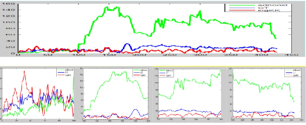
Figure 7 shows the estimated distances between the actual position and that obtained by

each method. The x-coordinate corresponds to the frame index, and the y-coordinate

corresponds to the distance (in pixels) between the tracking result by each method and the actual position. Until frame 50, sigKK (=SigKPF) looks somewhat unstable compared to that by RCT (=CT). However in the long run, sigKK works obviously better than RCT.

We also draw two results by sigKF and sigKP to see the effect of KalmanF and KalmanP.

Interestingly, the graph of sigKF is similar to that of RCT, improving only very little. On the other hand, even though sigKP sometimes gives worse results than RCT, it eventually gives a

better result and KalmanP seems to be more important than KalmanF. Anyhow they seem to

Figure 7. Comparison of the tracking results by different algorithms AdaBoost is a feature selection algorithm widely used in machine learning community, and it seems feasible to improve the performance of RCT by introducing AdaBoost in it. We obtained the AdaBoost code from [9], and created an online compressive AdaBoost tracker

(we name it OCA for short) by replacing RCT’s naïve Bayes classifier.

Figure 8 shows the comparison of the three algorithms, OCA (in green), RCT (in blue), and sigKK (in red). The four small figures in the lower part show magnified views for frames 1~100, 100~200, 200~300 and 300~426. Until frame 100, the performance of AdaBoost tracker is the best, while that of sigKK is the poorest. But after frame 100, sigKK shows the best performance until the end.

Probably one of the reasons why AdaBoost shows poor performance after frame 100 is, because the person in the video turned his head slightly, and AdaBoost did not have enough data for training as the shape of the object changes.

Figure 8. Comparison of the three algorithms using the data set [16] -

OCA (green), RCT (=CT,blue), and sigKK (red)

5. Conclusion and Future Work

In this paper, we proposed a tracking algorithm based on classification involving online feature selection. Our algorithm combines compressed representation and feature selection. Such a combination has been rarely used in other literatures. We introduced a feature valuation and weighting method to combine weaker classifiers to form a strong classification. This feature selection is independent of applications, and it can be combined with any representation of a feature space to train classifiers. We also introduced the Kalman filter to deal with the translation of object between two consecutive frames. Experimental results show that our assumption is feasible and the formulation based on estimation of

To realize successful longer term tracking, it seems that we need to perform more elaborate analysis to rank each feature’s discriminative power for a better discriminative feature basis. One of the directions might be employing the Fisher discriminant analysis to rank each feature’s discriminative power and combining with the AdaBoost algorithm. Our first try with AdaBoost was not successful, showing a better performance only at the beginning. We will focus on how to make AdaBoost keep such a good performance in long term tracking. Nonetheless, there always exists a tradeoff between accuracy and efficiency, which we need to balance on our way.

Acknowledgements

The authors would like to thank Dr. K. Zhang for making their precious videos publicly available with no restriction. They also thank Professor A. Li at Qilu University of Technology in China for making helpful discussion on their work. This work was supported by the GRRC program of Gyeonggi province [GRRC SUWON2013-B1, Cooperative CCTV Image Based Context-Aware Process Technology].

References

[1] D. Achlioptas, “Database-friendly random projections: Johnson-Lindenstrauss with binary coins”, J. Comput. Syst. Sci, vol. 66, no. 4, (2003), pp.671–687, doi: 10.1016/S0022-0000(03)00025-4.

[2] B. Babenko, M. -H. Yang and S. Belongie, “Robust object tracking with online multiple instance learning”, IEEE Tran. J. Pattern Analysis and Machine Intelligence, vol. 33, (2011) August, pp. 1619-1632.

[3] C. Bao, Y. Wu, H. Ling and H. Ji, “Real Time Robust L1 Tracker Using Accelerated Proximal Gradient Approach”, IEEE CVPR, (2012), pp. 1830 –1837.

[4] R. Collins, Y. Liu and M. Leordeanu, “On-Line Selection of Discriminative Tracking Features”, IEEE Transaction J. Pattern Analysis and Machine Intelligence, vol. 27, no. 10, (2005) October, pp.1631 –1643. [5] E. Cuevas, D. Zaldivar and R. Rojas, “Kalman Filter for Vision Tracking” Technical Report B, (2005). [6] P. Dollar, Z. Tu, H. Tao and S. Belongie, “Feature mining for image classification,” IEEE Conference on

CVPR’07, (2007) June, pp. 1-8.

[7] Z. Han, Q. Ye and J. Jiao, “Online Feature Evaluation for Object Tracking Using Kalman Filter”, Pattern Recognition, ICPR, (2008), pp. 1-4.

[8] Z. Kalal, J. Matas and K. Mikolajczyk, “P-N Learning: Bootstrapping Binary Classifiers by Structural Constraints”, CVPR, (2010).

[9] D. -J. Kroon, “AdaBoost algorithm”, http://www.mathworks.com/matlabcentral/fileexchange/27813-classic-AdaBoost-classifier.

[10] D. W. Liang, Q. M. Huang, W. Gao and H. X. Yao, “Online Selection of Discriminative Features Using Bayes Error Rate for Visual Tracking”, 7th Pacific-Rim Conference on Multimedia, (2006), pp. 547–555. [11] K. Okuma, A. Taleghani, N. D. Freitas, J. J. Little and D. G. Lowe, “Boosted Particle Filter: Multitarget

Detection and Tracking”, ECCV04, Part I, (2004) May, pp. 28-39, doi: 10.1007/978-3-540-24670-1_3. [12] S. Stalder, H. Grabner and L. van Gool, “Beyond Semi-Supervised Tracking: Tracking Should Be as Simple

as Detection, but not Simpler than Recognition”, IEEE ICCV Workshops, (2009) October, pp. 1409–1416. [13] J. Wang, X. Chen and W. Gao, “Online Selecting Discriminative Tracking Features Using Particle Filter”,

Proceedings of IEEE CVPR, vol. 2, (2005), pp. 1037–1042.

[14] A. Yilmaz, O. Javed and M. Shah, “Object tracking: A survey”, J. ACM Computing Surveys (CSUR), vol. 38, Issue 4, Article no.13, (2006), doi: 10.1145/1177352.1177355.

[15] K. Zhang, L. Zhang and M. Yang, “Real-Time Compressive Tracking”, ECCV, (2012).

K. Zhang, L. Zhang and M. Yang, “Real-time Compressive Tracking”, http://www4.comp.polyu.edu.hk/~cslzhang/CT/CT.htm.

Authors

Ye H. Chen is a lecturer at Information School of Qilu University of Technology, China. Her research interest includes computer vision, machine learning, image data mining, and algorithm design. She received her M.S. degree in Light Industry Machinery from Shaanxi University of Science and Technology, China.

Pil S. Park is a professor of Computer Science and the director of Information & Computer Center at University of Suwon, Korea. His research interest includes computer vision, especially tracking objects for surveillance, high performance computing, knowledge-based information systems, and Linux clusters. He received his Ph.D. in Interdisciplinary Applied Mathematics (with emphasis on Computer Science) from University of Maryland at College Park, M.S. in Applied Mathematics from Old Dominion University, U.S.A., and B.S. in Physical Oceanography from Seoul National University, Korea.