HAL Id: hal-02407684
https://hal.archives-ouvertes.fr/hal-02407684
Submitted on 12 Dec 2019
HAL
is a multi-disciplinary open access
archive for the deposit and dissemination of
sci-entific research documents, whether they are
pub-lished or not. The documents may come from
teaching and research institutions in France or
abroad, or from public or private research centers.
L’archive ouverte pluridisciplinaire
HAL, est
destinée au dépôt et à la diffusion de documents
scientifiques de niveau recherche, publiés ou non,
émanant des établissements d’enseignement et de
recherche français ou étrangers, des laboratoires
publics ou privés.
Is ensemble classifier needed for steganalysis in
high-dimensional feature spaces?
Rémi Cogranne, Vahid Sedighi, Jessica Fridrich, Tomas Pevny
To cite this version:
Rémi Cogranne, Vahid Sedighi, Jessica Fridrich, Tomas Pevny. Is ensemble classifier needed for
steganalysis in high-dimensional feature spaces?. 2015 IEEE International Workshop on Information
Forensics and Security (WIFS), 2015, Rome, Italy. �10.1109/wifs.2015.7368597�. �hal-02407684�
Is Ensemble Classifier Needed for Steganalysis in
High-Dimensional Feature Spaces?
R´emi Cogranne
ICD - LM2S - UMR 6281 CNRS Troyes University of Technology
Troyes, France [email protected]
Vahid Sedighi and Jessica Fridrich
Department of ECE Binghamton University Binghamton, NY 13902-6000 {vsedigh1,fridrich}@binghamton.eduTom´aˇs Pevn´y,
Department of Computers Czech Technical University in PraguePraha 6,166 27, Czech Republic [email protected]
Copyright c2015 IEEE. Personal use of this material is permitted. However, permission to use this material for any other purposes must be obtained from the IEEE by sending a request to [email protected]
Accepted version. Final to be published online on ieeex-plore.ieee.org within WIFS proceedings.
Abstract—The ensemble classifier, based on Fisher Linear Discriminant base learners, was introduced specifically for ste-ganalysis of digital media, which currently uses high-dimensional feature spaces. Presently it is probably the most used method to design supervised classifier for steganalysis of digital images because of its good detection accuracy and small computa-tional cost. It has been assumed by the community that the classifier implements a non-linear boundary through pooling binary decision of individual classifiers within the ensemble. This paper challenges this assumption by showing that linear classifier obtained by various regularizations of the FLD can perform equally well as the ensemble. Moreover it demonstrates that using state of the art solvers linear classifiers can be trained more efficiently and offer certain potential advantages over the original ensemble leading to much lower computational complexity than the ensemble classifier. All claims are supported experimentally on a wide spectrum of stego schemes operating in both the spatial and JPEG domains with a multitude of rich steganalysis feature sets.
Index Terms—Ensemble classifier, linear classifier, regulariza-tion, steganalysis, steganography.
I. INTRODUCTION
The objective of steganography is to hide a secret message within an innocuous looking cover object, such as a digital image, obtaining thus a stego object that can be sent overtly through an insecure channel. The related field that aims at detecting the presence of the hidden message is called steganalysis. Both fields have experienced a rapid development during the previous two decades [1].
Currently, the best detectors for modern steganographic methods are based on supervised learning; the general ap-proach consists of selecting a suitable set of features that
Copyright (c) 2015 IEEE. Personal use of this material is permitted. However, permission to use this material for any other purposes must be obtained from the IEEE by sending a request to [email protected]
Accepted version. Final to be published online on ieeexplore.ieee.org within WIFS proceedings.
can reveal the presence of hidden data, and then training a classifier using supervised machine learning, to distinguish between the classes of cover and stego features. To improve the detection accuracy of modern steganographic schemes, the feature dimension had to be substantially increased: re-cently proposed rich models may contain more than 30.000 features [4], [5]. This feature dimensionality (together with correspondingly large training sets) make it difficult to train the widely popular Gaussian Support Vector Machine (SVM), a popular choice among steganalysts before the introduction of rich media models.
The FLD ensemble classifier [6] has been proposed as a much more scalable alternative for classifier construction with large training sets and high dimensional feature spaces. This classifier is non-linear because of its employment of the ma-jority voting rule. Recently, it has recently been proposed [7] to replace the majority voting with a statistical test optimal within a multivariate Gaussian model of the base learners’ projections to achieve a better control over the error rates and to extend the ensemble training to unknown payload and multi-class steganalysis [8]. However, by doing so, the ensemble became a linear classifier. For binary classification measured using the classical minimal total classifier error under equal priors, the performance of this version of the ensemble was shown to be essentially the same as for the original ensemble. This observation motivated the current paper.
As recognized in [16], sub-space sampling in FLD ensemble can be viewed as a way to regularize the linear classifier. Thus, it makes sense to study other regularizations and compare their performance with the ensemble. The potential benefit is simplifying the training and lowering its complexity and potentially improving the performance when merging qualita-tively different feature spaces of highly unequal dimension.
The present paper is organized as follows. In Section II, we provide a brief description of the original FLD ensemble clas-sifier as well as its linear form cast within hypothesis testing theory. Then, in Section III introduces several approaches for regularizing linear classifiers as alternatives to the ensemble. The results of all numerical results appear in Section IV which includes wide spectrum of steganographic methods and with a diverse set of steganalysis features. Section V summarizes the present work and concludes the paper.
II. FLD ENSEMBLECLASSIFIER
To explain the contribution of this paper, in this section we review the original FLD ensemble as well as its recent linear reformulation. We use the following notational conventions. Matrices will be represented with capital bold letters X, vectors are denoted with lower case bold letters x, scalars with lower case lettersx, and sets and probability distributions with calligraphic capital letters X. The FLD ensemble clas-sifier was originally proposed [6] as an alternative to support vector machines, a scalable machine learning tool that can be efficiently used to build accurate detectors in high dimensional feature spaces and large training data sets. Since the FLD is a well-known tool, it is only briefly described in this section. The reader is referred to [9] for a more detailed presentation. Let f ∈ Rd be a (row) vector of d features extracted
from one image. Let the training sets of cover and stego image features be matrices of size Ntrn×d denoted Ctrn and Strn whose components are ctrn
n,i and strnn,i, respectively.
The FLD assumes that among these two classes, the features are i.i.d. with means µc and µs, row vectors of size 1×d,
and covariance matrices Σc andΣsof sized×d. Among all
linear decision rules defined by:
C:
(
H0 if f ·wT−b <0
H1 if f ·wT−b >0,
(1) where f is a feature (row) vector to be classified and b is a threshold, the FLD finds the vector of weights w ∈ Rd
that maximizes the following Fisher separability criterion (also called Fisher ratio):
F(w) =w(µc−µs)
T(µ
c−µs)wT
w(Σc+Σs)wT
. (2)
Few calculations show that the maximization of F(w)
from the training data, Ctrn andStrn, leads to the following weighting vector w: w= (µbs−µbc)Σbc+Σbs −1 (3) with µbci= 1 Ntrn Ntrn X n=1 ctrnn,i , bµsi = 1 Ntrn Ntrn X n=1 strnn,i , b Σcn,i= 1 Ntrn−1 Ntrn X n=1 (ctrnn,i−bµci)(c trn n,j−µbcj), and Σbsn,i= 1 Ntrn−1 Ntrn X n=1 (strnn,i−bµsi)(s trn n,j−µbsj).
In practice, the inversion of the “between class” covariance matrix, Σbc +Σbs, is seldom performed directly but almost
always using a regularization by adding λId to improve
numerical stability:Σbc+Σbs+λId, withIdthe identity matrix
of sized×d. In fact, when the feature-space dimensionalityd
is of a similar order of magnitude that the number of samples
Ntrn, the empirical between-class covariance matrix is often ill-conditioned.
The FLD ensemble is a set of L base learners imple-mented as FLDs trained on uniformly randomly selecteddsub -dimensional subsets F1, . . . ,FL of the feature space. This
approach to diversify base learners was firstly used with decision trees in [24]. The ensemble reaches its final decision by fusing the decisions of allLindividual base learners using majority voting. The ensemble training scales well w.r.t. the feature dimensionality and the training set size because one can selectdsub << d. The hyper-parameters dsub andL are determined by a search using either a cross-validation set or by bootstrapping (the latter choice was selected in the original publication [6]).
Recently [7], [8], the FLD ensemble was reformulated within the hypothesis testing theory. In particular, the majority voting rule was replaced with a likelihood ratio. Below, we briefly explain the main idea. Denoting the weight vector of the
ith base learner asw(i), we definev∈
RL,v= (v1, . . . , vL),
vi=f·w(i)T, the vector ofLprojections of the feature vector
f on allLweight vectors,w(1), . . . ,w(L). An assumption has been made about v that it follows a multivariate Gaussian (MVG) distributionN(µ0,Σ0)andN(µ1,Σ1)on cover and stego features. After normalizing the projection vector by
˜
v= (v−µ0)Σ0−1/2and under the shift hypothesisΣ0=Σ1,
˜
v∼ N(0,IL)andv˜ ∼ N(θ1,IL)on cover and stego images.
The majority voting decision can thus be replaced with a LRT in the form: L: ( H0 if Λlr(˜v)< τ H1 if Λlr(˜v)> τ, (4) where τ is a threshold that can be selected, for example, to maximize the test power while satisfying a prescribed false-alarm rate, and
Λlr(˜v) = θ1v˜
T
kθ1k2
, (5)
is the likelihood ratio. Note that, in contrast with the majority voting, this decision rule makes the classifier linear and the sole difference to the single FLD using all features is how the linear classifier is constructed.
III. FROMENSEMBLE TO LINEAR CLASSIFIER
As briefly summarized in the previous section, replacing the majority-voting rule in the FLD ensemble with a LRT turns the ensemble into a linear classifier. And, as shown in [7], [8], this linear classifier can achieve essentially the same performance as the non-linear FLD ensemble [6] at least in classification problems in steganalysis. Indeed, if the decision boundary in high-dimensional rich image models is close to linear, we will not see any large difference between linear and non-linear classifiers. Being aware of this caveat, we hypothesize that at least in current classification problems in digital image steganography, it appears that linear classifiers can achieve essentially the same classification accuracy as the original FLD ensemble employing majority voting. It thus becomes meaningful to ask whether there exist simpler approaches based on the FLD that use alternative methods for
its regularization that might offer advantages over the original ensemble, such as a lower training complexity.
To this end, we study the following four linear classifiers: an
`2regularization of the reciprocal Fisher ratio, ridge regression that is a least square estimation with `2 regularization, an alternative implementation of ridge regression using LSMR optimization method [11], and a least square estimation with
`1 regularization, known as LASSO.
`2 regularization of the Fisher ratio. This is achieved by replacing the maximization of the Fisher ratio (2) with
w= arg minF(w)−1+λkwk2
2. (6)
It is shown in Appendix that this`2regularization leads to the same weight vectorw as the vector obtained using Tikhonov regularization of the between-class covariance matrix (3):
w= (µbs−µbc)Σbc+Σbs+λId
−1
.
Ridge-regression, also referred to Tikhonov regularization based on least square estimation [10]. To formally describe this classifier, let us denote the matrix of all training samples:
X= Ctrn Strn ,
and, similarly, let us define the label vector y∈R2N
trn that represents the class of the samples from matrix X:
y=−1−1−1. . .−1−1 | {z } Ntrn 11. . .11 | {z } Ntrn T .
The ridge regression aims at finding a weighting vector wrr that minimizes the squared error between the label yand the linearly estimated label:
wrr= arg min w∈Rd ky−X wTk2 2+λkwk 2 2. (7)
Few calculations show that, see for instance [10], that an explicit solution of Eq. (7) is given by:
wrr = (XTX+λId)−1XTy.
Interestingly, the weighting vector given by the ridge regres-sion corresponds to the weighting vector of the regularized FLD provided that the features have a zero-mean (see Ap-pendix A). We note however that, because we did not center the features, the solution of the ridge regression does not correspond to the weighting vector of the regularized FLD.
Solving linear least square with LSMR. Note that all optimization problems above can be obtained by solving the appropriate system of linear equations. The main advantage of this approach is the fact that there exist numerous optimization methods for solving large linear systems efficiently. These methods are iterative and are associated with a stopping criterion either on the solutionwrror the residual y−X w0rr. To this end, we implemented the ridge regression using a large linear system optimization method called LSMR [11] due to its low computational complexity and low memory requirements.1
1LSMR (Least Square Minimun-Residual) function can be downloaded
from Stanford University’s Systems Optimization Laboratory.
We note that this approach needs to find two parameters – the regularization parameter λ and the tolerance used in LSMR, which controls the trade off between computational efficiency and optimality of the found solution. In this paper, we simply fix λ = 10−8 (as we saw negligible sensitivity w.r.t. this parameter) and search for the tolerance to obtain the best detection accuracy.
LASSO regularization, Equations (7) and (6) can be viewed as`2regularized optimizations. The machine learning community frequently uses an `1 regularization because it has the added benefit of producing sparse solutions (solutions where only some items ofware non-zero), thus identifying a sufficient set of features for linear classifiers (`1regularization is also called the Least Absolute Shrinkage and Selection Operator (LASSO)). In this work, we used`1in Eq. (7), which leads to the following minimization problem:
arg minky−X wTk2
2+λkwk1. (8) While there is no analytic solution to the LASSO regulariza-tion problem (8), efficient convex optimizaregulariza-tion methods can be applied [25].2
IV. NUMERICAL RESULTS
Before discussing the numerical results, we briefly present the common core of all experiments.
All results presented in this paper are obtained on BOSSbase 1.01 [12] of10,000 512×512gray-scale images. For gener-ality, both spatial domain and JPEG domain steganographic schemes have been used together with spatial domain and JPEG domain feature sets.3 For spatial domain, four embed-ding algorithms have been used, namely, HUGO [13] with bounding distortion (HUGO-BD), Wavelet Obtained Weights (WOW) [14], Spatial UNIversal WAvelet Relative Distortion (S-UNIWARD) [2], and the recent scheme based on statistical detectability [15], [17]. For steganalysis, we used four spatial domain feature sets: the second-order Subtractive Pixel Adja-cency Matrix (SPAM) [3] of dimensionality 686, the Spatial Rich Model (SRM) [4] as well as its selection-channel-aware version (maxSRM) [18], both made of 34,671 features, and the version with a single quantization (SRMQ1) containing
12,753features.
For the JPEG domain, we used both non-side informed algo-rithms and side-informed algoalgo-rithms. For the first type, we used nsF5 [19], Entropy-Based Steganography (EBS) [20], Uniform Embedding Distortion (UED) [21], and JPEG do-main UNIWARD [2],referred to as J-UNIWARD. Three algo-rithms have been used for side-informed JPEG steganography: Perturbed Quantization (PQ) [19], the side-informed version of EBS (EBS) [20], and side-informed UNIWARD, SI-UNIWARD [2]. Five feature set that target JPEG domain embedding have been used: CF? [6], of dimension 7,850,
the Cartesian-calibrated JPEG Rich Model (CC-JRM) [5] used alone and used in union with SRMQ1, referred to as JSRM [5],
2In the present paper we used MatlabR lasso function.
3All feature extractors and most embedding algorithms used can be
10−1010−9 10−8 10−7 10−6 10−5 10−4 10−3 10−2 10−1 100 0.2 0.3 0.4 0.5 Ensemble MV PE FLD LASSO Ridge-reg. LSMR
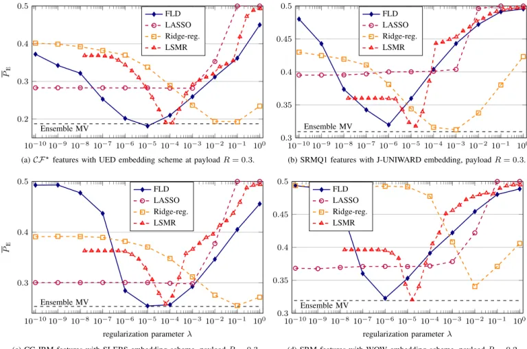
(a)CF?features with UED embedding scheme at payloadR= 0.3.
10−1010−9 10−8 10−7 10−6 10−5 10−4 10−3 10−2 10−1 100 0.3 0.35 0.4 0.45 0.5 Ensemble MV FLD LASSO Ridge-reg. LSMR
(b) SRMQ1 features with J-UNIWARD embedding, payloadR= 0.3.
10−1010−9 10−8 10−7 10−6 10−5 10−4 10−3 10−2 10−1 100 0.3 0.4 0.5 Ensemble MV regularization parameterλ PE FLD LASSO Ridge-reg. LSMR
(c) CC-JRM features with SI-EBS embedding scheme, payloadR= 0.3.
10−1010−9 10−8 10−7 10−6 10−5 10−4 10−3 10−2 10−1 100 0.3 0.35 0.4 0.45 0.5 Ensemble MV regularization parameterλ FLD LASSO Ridge-reg. LSMR
(d) SRM features with WOW embedding scheme, payloadR= 0.2.
Fig. 1: Evolution ofPEas a function of the regularization parameterλ(or tolerance of LSMR) for several embedding algorithms
and several feature sets.
whose dimensionality is 35,263, the recent Discrete Cosine Transform Residual (DCTR) [22], consisting of8,000features based on undecimated DCT coefficients, and the PHase Aware pRojection Model (PHARM) [23], made of 12,600features.
In this paper, the detection accuracy is measured as the total probability of error under equal Bayesian priors PE =
1/2(PF A+PM D), with PF A and PM D the empirical prob-ability of false alarm and missed detection respectively. The detection accuracy is also always averaged over 10 splits on the testing set (a 50/50 split for training and testing was used). First, Figure 1 contrasts the detection accuracy of the proposed linear classifier with the ensemble classifier. We note that the detection accuracy PE is plotted as a function
of the regularization parameter λ. Note that, as explained in the previous section, for the ridge-regression, that uses the LSMR large linear system optimization, we search for the tolerance, which controls the stopping criterion of the iterative minimization search, since the regularization parameterλhas negligible influence for this methods. Four different cases with different steganographic algorithms and feature sets are presented in Figure 1. The conclusions that follow can be observed across other combinations of feature sets and
embed-ding algorithms. First, note that the LASSO performs poorly in general but has the important advantage to be rather insensitive to the regularization parameters: the detection accuracy is almost always at its best for λ ∈ (10−15,10−5). Similarly, we note that both the FLD classifier and the ridge regression with a large system optimization can achieve roughly similar performance as the ensemble classifier. We also note that the FLD classifier almost always achieves the best detection accuracy for λ≈10−6; this fact can be used when searching for the best regularization parameter in cross-validation. On the other hand, the regularization parameter for which the the ridge regression, as well as its approximation, achieve the lowestPE depends on the feature set and the steganographic
algorithm.
Except for LASSO, for which we set λ = 10−10, the optimal value of the regularization parameter (or tolerance for LSMR) was determined by a simple grid search. For the large linear system optimization for ridge regression, because it has a very low computational complexity, we modified the code so that it outputs the solutions obtained for various tolerance values. This allowed us to keep the same computational complexity as the smallest tolerance value, which we set
TABLE I: Detection accuracy of the ensemble classifier compared with the proposed linear classifiers for various embedding schemes. Detection accuracy is measured as total probability of errorPE.
Embedding algorithm / feature set Ensemble classifier [6] FLD classifier Ridge Regression LSMR Optimization [11] LASSO HUGO-BD [13],R= 0.2/ SPAM [3] .4409±.0021 .4414±.0017 .4409±.0021 .4405±.0027 .4598±.0015 S-UNIWARD [2],R= 0.2/ SRMQ1 [4] .3283±.0033 .3364±.0029 .3450±.0211 .3342±.0029 .3671±.0038 WOW [14],R= 0.2/ SRM [4] .3196±.0031 .3289±.0021 .3402±.0039 .3267±.0023 .3694±.0051 MiPOD [15],R= 0.2/ maxSRMd2 [18] .3237±.0038 .3321±.0036 .3343±.0101 .3307±.0029 .3669±.0048 UED [21],R= 0.3/CF?[6] .1890±.0043 .2181±.0823 .1909±.0046 .1925±.0049 .2875±.0047 J-UNIWARD [2],R= 0.3/ SRMQ1 [5] .3112±.0045 .3197±.0032 .3317±.0074 .3185±.0023 .3950±.0034 UED [21],R= 0.2/ PHARM [23] .1742±.0034 .4950±.0041 .4959±.0026 .1748±.0024 .5000±.0000 SI-UNIWARD [2],R= 0.4/ DCTR [22] .4261±.0029 .4355±.0196 .4292±.0041 .4298±.0021 .4899±.0135 SI-EBS [20],R= 0.3/ CCJRM [5] .2517±.0035 .2608±.0025 .2614±.0061 .2592±.0023 .3019±.0042 SI-UNIWARD [2],R= 0.3/ JSRM [5] .4582±.0020 .4630±.0026 .4608±.0030 .4616±.0031 .4764±.0042
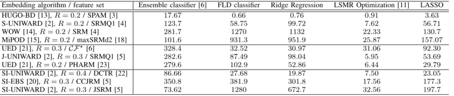
TABLE II: Computation time (in seconds) of the ensemble classifier compared with the proposed linear classifiers, same settings as in Table I. Computations were carried out on a 16-physical-core IntelR XeonR E5 @ 2.60GHz with RAM 256GB.
Embedding algorithm / feature set Ensemble classifier [6] FLD classifier Ridge Regression LSMR Optimization [11] LASSO
HUGO-BD [13],R= 0.2/ SPAM [3] 17.67 0.66 0.76 0.91 3.63 S-UNIWARD [2],R= 0.2/ SRMQ1 [4] 123.7 58.75 99.72 7.62 56.71 WOW [14],R= 0.2/ SRM [4] 281.7 1270 1132 22.33 130.7 MiPOD [15],R= 0.2/ maxSRMd2 [18] 101.6 931.3 951.9 25.87 157.07 UED [21],R= 0.3/CF?[6] 328.4 32.52 30.97 31.06 92.30 J-UNIWARD [2],R= 0.3/ SRMQ1 [5] 282.6 87.49 98.04 5.95 53.69 UED [21],R= 0.2/ PHARM [23] 279.6 102.9 52.86 6.44 29.79 SI-UNIWARD [2],R= 0.4/ DCTR [22] 86.66 27.68 19.87 7.50 23.05 SI-EBS [20],R= 0.3/ CCJRM [5] 350.8 381.9 301.8 17.56 177.3 SI-UNIWARD [2],R= 0.3/ JSRM [5] 73.62 1280 672.7 32.56 197.7
to 10−6 in this paper, as this corresponds to the case with highest number of iterations. A larger value may be used to further decrease the computational time, see Figure 1). The tolerance value for which thePEis the smallest on the
cross-validation subset is used for testing. For the FLD and the ridge regression, the computational time is slightly lower for larger regularization parameters. Hence, we start the one dimensional search with a rather large regularization parameter, typically
λ = 10−6 for the FLD and λ = 10−1 for ridge regression. However, the implementation has to be a trade-off between computational time and detection accuracy. For the FLD and ridge-regression (using off-the-shelf solver) we wanted to keep the computational time manageable, though sometimes rather important, as the cost of poor convergence in few cases, see for instance the results obtained for UED embedding scheme and PHARM features in Table I. We would like to acknowledge that this implementation of the linear classifier may certainly be largely improved. Nevertheless, the results presented in Tables I and II show that even such simplistic approaches already show very promising results.
Table I compares the detection accuracy of the ensemble classifier (with optimal values of dsub and L), the FLD, the ridge regression, and the large system optimization for ridge regression using the LSMR and the LASSO. All these classifiers were used with the optimally found regularization parameterλ(or tolerance) as described above. Table I shows that for a majority of the cases, the linear classifiers perform slightly worse than the ensemble classifier: the difference in terms ofPE is between0.05% and0.8%for ridge regression
implemented using LSMR optimization algorithm. Note also that the LASSO always performs significantly worse.
Table II compares the computational time of the same clas-sifiers with the same settings. Note that for feature sets of medium dimensionality (typically up to15,000 features) the ensemble classifier always requires a much higher computa-tional time than all its competitors. However, for larger feature sets (see the results with SRM, maxSRM, CC-JRM, and JSRM) the computational time of FLD and ridge regression as well as the memory requirements become prohibitively large since a very large matrix has to be stored and inverted. In fact, most of the computational time of both the FLD and ridge regression come from the inversion of a matrix of sized×d, which has the complexityO(d3). Let us recall, for comparison, that the ensemble has a complexity O(NtrnLd2sub+Ld3sub). By contrast we note that the ridge regression solved using LSMR iterative optimization methods has a complexity of
O(NitNtrn×d), withNit the number of iterations [11]. This should be contrasted with the loss of detection accuracy.
V. CONCLUSION
The main contribution of this paper is to show that the power of the FLD ensemble classifier widely used in steganalysis does not come from the non-linearity of the majority voting rule but from the natural regularization process of the ensemble when training on random subsets of features. This paper also shows that, if correctly regularized, a simple FLD classifier or a ridge regression may achieve almost the same performance. However, their naive implementation by using off-the-shelf solvers (e.g. in Matlab) leads to very high complexity for large feature sets. As a remedy, we have demonstrated on ridge regression that state-of-the-art optimization algorithms allow us to achieve almost the same detection accuracy as an
ensemble classifier for a computational time up to 10 times smaller. Further work can be done to further improve the detection accuracy and the computational complexity.
ACKNOWLEDGEMENTS
Vahid Sedighi and Jessica Fridrich were supported by Air Force Office of Scientific Research under the research grant number FA9950-12-1-0124. The U.S. Government is autho-rized to reproduce and distribute reprints for Governmental purposes notwithstanding any copyright notation there on. The views and conclusions contained herein are those of the au-thors and should not be interpreted as necessarily representing the official policies, either expressed or implied of AFOSR or the U.S. Government. The work of R´emi Cogranne was funded in part by the STEG-DETECT program for scholar mobility and by IDENT research grant both from Conseil Rgional de Champagne-Ardenne.
APPENDIX
REGULARIZATION OFFLD
In this appendix, we show that an L2-regularization of the reciprocal Fisher ratio, which is the optimization problem:
arg minwF(w)−1+λkwk
2
, is equivalent to regularizing the between class covariance matrix Σ = Σc+Σs in classical
FLD by adding λ0Id to it before inversion.
To this end, we write the reciprocal Fisher ratio (2) as
1/F(w) =wΣwT/wΓwT, where we used for compactness Γ= (µc−µs)T(µ
c−µs). We note that from the definition
of Γ,ΓxTis a multiple of (µ
c−µs)Tfor any vector x. We
now differentiate the objective function w.r.t. w to find the minimum: d dw F(w)−1+λw·wT 2 = ΣwTwΓwT−ΓwTwΣwT (wΓwT)2 +λw. Setting this expression to zero and multiplying by wΓwT gives us an equation for w
(Σ+λa2(w))wT=c(w)(µc−µs)T, (9)
where a(w) =w(µc−µs)Tand c(w) =wΣwT/a(w) are scalars. Since wcan be normalized so thata(w) = 1, Eq. (9) the projection vector w is obtained by
w= (Σ+λ)−1(µc−µs)T,
which is the same as the regularization of the inverse covari-ance Σ in classical FLD.
APPENDIX
RELATIONSHIP BETWEEN LEAST-SQUARE ANDFLD This appendix recalls the relationship between ridge regres-sion and FLD. The FLD projection vector w is given by :
w= (µbs−µbc) (Σbc+Σbs)−1.
The mean of cover features may be easily obtained by b
µc= N1CtrnT·1
N with1N a (column) vector of ones. Hence,
recalling that the matrix of all training data is:X=
Ctrn
Strn
,
and recalling that it is assumed, without loss of generality, that the label for cover is1and−1for stego, it is straightforward that: (µbc−µbs) T = 1 NX TY.
Additionally, assuming, without loss of generality, that the features are normalized so that the columns of X have a zero mean, or equivalently µbc = −µbs, it is then obvious (by a block-wise matrix product) that XTX =
CtrnTCtrn+StrnTStrn
= (N−1)Σbc+Σbs
Thus the linear least square regression (XTX)−1XTY can be rewritten, up to a scaling factor, as:
(µbc−µbs)Σbc+Σbs
−1
.
REFERENCES
[1] A. D. Ker, P. Bas, R. B¨ohme, R. Cogranne, S. Craver, T. Filler, J. Fridrich, and T. Pevn´y, “Moving steganography and steganalysis from the laboratory into the real world,” in ACM Information hiding and multimedia security, IH&MMSec’13, 2013, pp. 45–58.
[2] V. Holub, J. Fridrich, and T. Denemark, “Universal distortion function for steganography in an arbitrary domain,” EURASIP Journal on Information Security, vol. 2014, no. 1, pp. 1–13, 2014.
[3] T. Pevn´y, P. Bas, and J. Fridrich, “Steganalysis by subtractive pixel adjacency matrix,”IEEE Trans. Inform. Forensics and Security, vol. 5, no. 2, pp. 215–224, 2010.
[4] J. Fridrich and J. Kodovsk`y, “Rich models for steganalysis of digital images,” Information Forensics and Security, IEEE Transactions on, vol. 7, no. 3, pp. 868 –882, june 2012.
[5] J. Kodovsk`y and J. Fridrich, “Steganalysis of JPEG images using rich models,”in IS&T/SPIE Electronic Imaging conf., vol. 8303, 2012, pp. 83 030A–13.
[6] J. Kodovsk`y, J. Fridrich, and V. Holub, “Ensemble classifiers for steganalysis of digital media,”Information Forensics and Security, IEEE Transactions on, vol. 7, no. 2, pp. 432–444, April 2012.
[7] R. Cogranne, T. Denemark, and J. Fridrich, “Theoretical model of the FLD ensemble classifier based on hypothesis testing theory,” in IEEE International Workshop on Information Forensics and Security (WIFS), 2014, pp. 167–172.
[8] R. Cogranne and J. Fridrich, “Modeling and extending the ensemble classifier for steganalysis of digital images using hypothesis testing the-ory,”(accepted for publication in) Information Forensics and Security, IEEE Transactions on, 2015.
[9] R. O. Duda, P. E. Hart, and D. G. Stork,Pattern classification, 2nd ed. John Wiley & Sons, 2012.
[10] T. Hastie, R. Tibshirani, J. Friedman, and J. Franklin, The elements of statistical learning: data mining, inference and prediction, 2nd ed., Springer, 2009.
[11] D. C.-L. Fong and M. Saunders, “LSMR: An iterative algorithm for sparse least-squares problems,”SIAM Journal on Scientific Computing, vol. 33, no. 5, pp. 2950–2971, 2011.
[12] P. Bas, T. Filler, and T. Pevn´y, “Break our steganographic system — the ins and outs of organizing boss,” inInformation Hiding, ser. LNCS vol.6958, 2011, pp. 59–70.
[13] T. Pevn`y, T. Filler, and P. Bas, “Using high-dimensional image models to perform highly undetectable steganography,” inInformation Hiding, ser. LNCS vol. 6387, 2010, pp. 161–177.
[14] V. Holub and J. Fridrich, “Designing steganographic distortion using directional filters,” in IEEE International Workshop on Information Forensics and Security (WIFS), 2012, pp. 234–239.
[15] V. Sedighi, J. Fridrich, and R. Cogranne, “Content-adaptive pentary steganography using the multivariate generalized gaussian cover model,” IS&T/SPIE Electronic Imaging conf., vol. 9409, 2015, pp. 94 090H. [16] T. Pevn`y, A. D. Ker’, “Towards dependable steganalysis,”IS&T/SPIE
Electronic Imaging conf., vol. 9409, 2015, pp. 94 090I.
[17] V. Sedighi, R. Cogranne, and J. Fridrich, “Content-Adaptive Steganogra-phy by Minimizing Statistical Detectability,”Information Forensics and Security, IEEE Transactions on(submitted).
[18] T. Denemark &al., V. Sedighi, V. Holub, R. Cogranne, and J. Fridrich, “Selection-channel-aware rich model for steganalysis of digital images,” inIEEE International Workshop on Information Forensics and Security (WIFS), 2014, pp. 48–53.
[19] J. Fridrich, T. Pevn´y, and J. Kodovsk´y, “Statistically undetectable JPEG steganography: Dead ends challenges, and opportunities,” inACM 9th workshop on Multimedia & security, MMSec’07, 2007, pp. 3–14. [20] C. Wang and J. Ni, “An efficient JPEG steganographic scheme based
on the block entropy of DCT coefficients,” in IEEE International Conference on Acoustics, Speech and Signal Processing (ICASSP), 2012, pp. 1785–1788.
[21] L. Guo, J. Ni, and Y. Q. Shi, “An efficient JPEG steganographic scheme using uniform embedding,” inIEEE International Workshop on Information Forensics and Security (WIFS), 2012, pp. 169–174. [22] V. Holub and J. Fridrich, “Low-complexity features for JPEG
steganalysis using undecimated DCT,” Information Forensics and Security, IEEE Transactions on, vol. 10, no. 2, pp. 219–228, Feb 2015. [23] ——, “Phase-aware projection model for steganalysis of JPEG images,”
IS&T/SPIE Electronic Imaging conf., vol. 9409, 2015, pp. 94 090T. [24] T. K. Ho, “Random decision forests” inProc. of International Conf. on
Document Analysis and Recognition, pp. 278–282, 1995.
[25] R. Tibshirani, “ Regression shrinkage and selection via the lasso”, Journal of the Royal Statistical Society, Series B, Vol 58, No. 1, pp. 267–288, 1996.