Biplot methodology for analysing and evaluating missing multivariate nominal scaled data

(1)

evaluating

missing

multivariate

nominal

scaled

data

Submitted

by

JOHANÉ

NIENKEMPER

‐

SWANEPOEL

Dissertation

presented

for

the

degree

of

Doctor

of

Philosophy

in

the

Department

of

Statistics

and

Actuarial

Science

in

the

Faculty

of

Economic

and

Management

Sciences

at

Stellenbosch

University.

Supervisor:

Professor

NJ

le

Roux

Co

‐

supervisor:

Professor

S

Gardner

‐

Lubbe

(2)

Declaration

By submitting this dissertation electronically, I declare that the entirety of the work contained

therein is my own, original work, that I am the sole author thereof (save to the extent explicitly

otherwise stated), that reproduction and publication thereof by Stellenbosch University will

not infringe any third party rights and that I have not previously in its entirety or in part

submitted it for obtaining any qualification.

Johané Nienkemper‐Swanepoel

Date: December 2019

Signature: (Declaration with signature in possession of candidate and supervisors.)

(3)

Abstract

This research aims at developing exploratory techniques that are specifically suitable for

missing data applications. Categorical data analysis, missing data analysis and biplot

visualisation are the three core methodologies that are combined to develop novel

techniques. Variants of multiple correspondence analysis (MCA) biplots are used for all

visualisations.

The first study objective addresses exploratory analysis after multiple imputation (MI).

Multiple plausible values are imputed for each missing observation to construct multiple

completed data sets for standard analyses. Biplot visualisations are constructed for each

completed data set after MI which require individual exploration to obtain final inference.

The number of MIs will greatly affect the accuracy and consistency of the interpretations

obtained from several plots. This predicament led to the development of GPAbin, to optimally

combine configurations from MIs to obtain a single configuration for final inference. The

GPAbin approach advances from two statistical techniques: generalised orthogonal

Procrustes analysis (GPA) and the combining rules used to combine estimates obtained from

MIs, Rubin’s rules.

Albeit a superior missing data handling approach, MI could be daunting for the non‐technical

practitioner. Therefore, an adequate alternative approach could be appealing and contribute

to the variety of available methods for the handling of incomplete multivariate categorical

data. The second objective aims at confirming whether visualisations obtained from non‐

imputed data sets are a suitable alternative to visualisations obtained from MIs. Subset MCA

(sMCA) distinguishes between observed and missing subsets of a multivariate categorical data

set by creating an additional response category level (CL) for missing responses in the

indicator matrix. Missing and observed responses can be visualised separately by only

considering the subset of interest in the recoded indicator matrix. The visualisation of the

observed responses utilises all available information which would have been forfeited by

deletion methods.

The third study objective explores the possibility of predicting a complete multivariate

categorical data set from MI visualisations obtained from the first study objective. The

(4)

responses. Since the aim of this research is to advance missing data visualisations, the

visualisations obtained from predicted completed data sets are compared to visualisations of

simulated complete data sets. The emphasis is on preserving inference and not recreating the

original data.

Missing data techniques are typically developed to address a specific missing data problem.

It is therefore crucial to understand the cause of missingness in order to apply suitable missing

data techniques. The fourth study objective investigates the sMCA biplot of the missing subset

of the recoded indicator matrix. Configurations of the incomplete subsets enable the

recognition of non‐response patterns which could provide insight into the particular missing

data mechanism (MDM). The missing at random (MAR) MDM refers to missing responses that

are dependent on the observed information and is expected to be identified by patterns and

groupings occurring in the incomplete sMCA biplot. The missing completely at random

(MCAR) MDM states that all observations have the same probability of not being captured

which could be identified by a random cloud of points in the incomplete sMCA biplot. Cluster

analysis is applied to confirm distinguishable groupings in the incomplete sMCA biplot which

could be used as a guideline to identify the MDM.

The proposed methodologies to address the different study objectives are evaluated by

means of an extensive simulation study comprising of various sample sizes, variables and

varying number of CLs which are simulated from three different distributions. The findings of

the simulation study are applied to a real data set to aid as a guide for the analysis.

Functions have been developed for R statistical software to perform all methodology

presented in this research. It is included as a tool pack provided as an appendix to assist in

the correct handling and unbiased visualisation of multivariate categorical data with missing

observations.

Keywords: biplots; categorical data; missing data; multiple correspondence analysis; multiple

(5)

Opsomming

Die doel van hierdie navorsing is om verkennende tegnieke te ontwikkel wat spesifiek vir

ontbrekende data geskik is. Kategoriese data‐analise, ontbrekende data‐analise en bi‐stipping

visualisering is die drie kern metodologieë wat gekombineer word om nuwe tegnieke te

ontwikkel. Variante van meervoudige ooreenkomsanalise bi‐stippings word gebruik vir alle

visualiserings.

Die eerste doelstelling fokus op die verkennende analise van datastelle nadat meervoudige

imputasie uitgevoer is. Meervoudige realistiese waardes word vir elke ontbrekende waarde

ingevul om sodoende meervoudige voltooide datastelle te konstrueer vir verdere standaard

analises. Bi‐stipping visualiserings word vir elke voltooide datastel na ‘n meervoudige

imputasie gekonstrueer. Aparte verkenning van die individuele visualiserings word vereis om

‘n finale inferensie te verkry. Die aantal meervoudige imputasies sal die akkuraatheid en

konsekwentheid van die interpretasies van verskeie stippings beïnvloed. Hierdie probleem

het tot die ontwikkeling van die GPAbin metode gelei om die meervoudige visualiserings van

meervoudige imputasies optimaal in een figuur vir ‘n finale inferensie te kombineer. Die

GPAbin metode vloei uit twee statistiese tegnieke voort: veralgemeende ortogonale

Procrustes analise en Rubin se reëls vir die samevoeging van beramings.

Alhoewel meervoudige imputasie bo ander tegnieke vir die hantering van ontbrekende data

verkies word, kan meervoudige imputasie uitdagend vir die nie‐tegniese gebruiker wees. ‘n

Voldoende alternatiewe tegniek kan aanloklik wees en tot die verskeidenheid van beskikbare

metodes vir die hantering van ontbrekende data bydra. Die tweede doelstelling poog dan juis

om vas te stel of visualiserings van nie‐geïmputeerde datastelle ‘n geskikte alternatief vir

visualiserings van meervoudige imputasies is. Sub‐meervoudige ooreenkomsanalise

onderskei tussen waargenome en ontbrekende deelversamelings van ‘n meerveranderlike

kategoriese datastel deur ekstra respons kategorievlakke vir ontbrekende waarnemings in die

indikatormatriks te skep. Ontbrekende en waargenome response kan apart gevisualiseer

word deur spesifieke deelversamelings in die indikatormatriks in ag te neem. Die visualisering

van waargenome response benut alle beskikbare inligting, dus word geen inligting verbeur

(6)

Die derde doelstelling ondersoek die moontlikheid om ‘n meerveranderlike kategoriese

datastel te voorspel vanaf meervoudige imputasie visualiserings wat in die eerste doelstelling

verkry is. Die afstand tussen die koördinate van ‘n bi‐stipping in die volle ruimte word gebruik

om realistiese responswaardes te voorspel. Aangesien die doel van hierdie navorsing is om

visualiserings vir ontbrekende data te bevorder, sal die visualiserings wat van ‘n voorspelde

datastel verkry word met die visualiserings van die oorspronklike gesimuleerde datastelle

vergelyk word. Die behoud van die oorspronklike inferensie is van belang en nie die

herskepping van die volledige oorspronklike data nie.

Tegnieke vir ontbrekende data word vir spesifieke ontbrekende data probleme ontwikkel. Dit

is dus noodsaaklik om die oorsaak van die ontbrekenheid te verstaan om sodoende toepaslike

ontbrekende data tegnieke toe te pas. Die vierde doelstelling fokus op die ontbrekende

deelversameling van die sub‐meervoudige ooreenkomsanalise bi‐stipping deur die

gekodeerde indikatormatriks te gebruik. Visualiserings van die onvolledige deelversamelings

maak die herkenning van nie‐respons patrone moontlik wat insig rakende die spesifieke

ontbrekende data meganisme verskaf. Die ewekansig ontbrekende meganisme verwys na

ontbrekende waarnemings wat afhanklik is van die waargenome responswaardes. Dit word

verwag dat hierdie meganisme sal lei tot patrone en groeperings in die sub‐meervoudige

ooreenkomsanalise bi‐stipping van die ontbrekende deelversameling. Wanneer alle

waarnemings dieselfde waarskynlikheid het om te ontbreek of waargeneem te word, word

dié meganisme as die algeheel ewekansig ontbrekende meganismse geklassifiseer. Aangesien

ontbrekende waardes onafhanklik van die waargenome waardes is, word dit verwag dat

hierdie meganisme geen merkbare patrone sal voortbring in die sub‐meervoudige

ooreenkomsanalise bi‐stipping nie. Trosanalise word toegepas om vas te stel of die visuele

groeperings betekenisvol van mekaar geskei kan word in die deelversameling sub‐

ooreenkomsanalise bi‐stipping geskei. Die graad van skeiding in die visualisering kan as ‘n

riglyn gebruik word om die ontbrekende data meganisme te identifiseer.

Die voorgestelde metodologieë om die verskillende doelwitte van hierdie studie aan te

spreek, word deur middel van ‘n omvangryke simulasie studie geëvalueer. Die simulasie

studie bevat datastelle met ‘n verskeidenheid van steekproefgroottes, aantal veranderlikes

(7)

Die bevindings van die simulasie studie word toegepas op ‘n bestaande datastel en dien as ‘n

gids vir die analise daarvan.

Funksies vir R statistiese sagteware is ontwikkel om alle metodes in hierdie navorsing te kan

uitvoer. Dit word as ‘n gereedskappakket in die bylae gegee om bystand te bied vir die

korrekte hantering en onsydige visualisering van meerveranderlike kategoriese data met

ontbrekende waardes.

Sleutelwoorde: bi‐stippings; kategoriese data; meervoudige imputasie; meervoudige

ooreenkomsanalise; ontbrekende data; Procrustes analise.

(8)

Acknowledgements

I wish to express my sincere gratitude and appreciation to the following persons and

institutions:

 My Creator for blessing me with talents and equipping me for any and all obstacles on

my path. Thank you, Holy Spirit, for Your continuous guidance in everything that I

pursue. In You and through You I am able.

Psalm 37:3‐4 Afrikaanse Bybel 1983 Vertaling

 My supervisors, Prof. Niël le Roux and Prof. Sugnet Lubbe.

I will always be indebted to you for the time you have invested in my future. Thank

you for sharing your knowledge and for always being available, your support have no

bounds. Thank you for your holistic approach to supervision and also taking my well‐

being into consideration. Thank you for creating opportunities to include me in the

exciting and evolving applications of multivariate data visualisations.

Prof. le Roux, thank you for noticing my potential since our first encounter in 2013 and

taking me under your ‘wing’.

 My husband, Franré. Thank you for being my partner in every challenge and

celebration. Thank you for being invested in my research and always believing that the

completion of this dissertation was within reach. Thank you for your immeasurable

love and support.

 My support system:

o Dorothy (my mother), Johan (my father) and Marisan (my sister).

Thank you for our daily conversations, your endless encouragement, moral support,

unconditional love and for always being proud of me.

A special thank you to my mother for imparting her love of research to me. Thank you

for taking the time to read through this dissertation.

 My extended family and friends for your ongoing support and prayers.

(9)

 Computations for the simulation study were performed using the University of

Stellenbosch’s HPC1 (Rhasatsha) and the University of Stellenbosch Central Analytical

Facilities’ HPC2 (CAF‐HPC1): http://www.sun.ac.za/hpc. A special thank you to

Gerhard Van Wageningen for his tireless technical assistance.

 Mr. Johan van Rooyen and Mr. Chris Bosman for setting up a virtual machine for

computationally intensive tasks which I could access remotely.

 The Teaching Development Grant National Collaborative Project for securing funding

for a study leave opportunity of six months in 2018.

 Dr. Rachelle Bester for her assistance to utilise the HPC clusters.

 Dr. Marietjie Vosloo for taking responsibility of my modules and presenting lectures

during my study leave.

 Mr. Morney Engelbrecht for alleviating my administrative responsibilities in the final

two years of my PhD and for always showing interest in my progress.

 The department of Genetics and the Faculty of AgriScience for granting me study leave

opportunities during my PhD and accommodating my research responsibilities.

 To the examiners for their time and positive feedback.

(10)

List of Figures

Figure 2.1 Bigraph of five samples (circles) and two categorical variables (squares: two CLs and

triangles: three CLs). ... 18

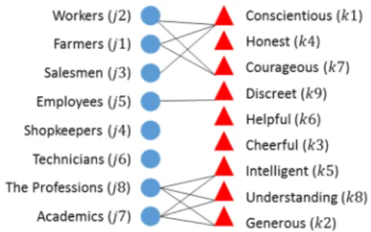
Figure 2.2 Attraction graph of professions (circles) and qualities (triangles). ... 18

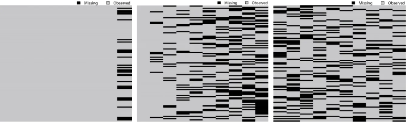
Figure 3.1 Missing data patterns. Left panel: Univariate pattern. Middle panel: Monotone pattern. Right panel: Arbitrary pattern. ... 42

Figure 3.2 Illustration of the steps of MI ... 51

Figure 4.1 Schematic representation of the GPAbin objective (cf. 1.4.1). ... 60

Figure 4.2 Schematic representation of the sMCA objective (cf. 1.4.2). ... 61

Figure 4.3 Schematic representation of the prediction objective (cf. 1.4.3). ... 62

Figure 4.4 Schematic representation of the MDM objective (cf. 1.4.4). ... 63

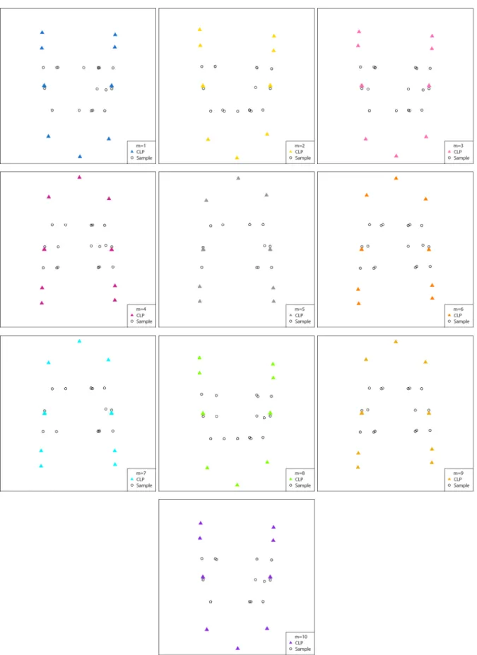
Figure 4.5 Illustration of MCA biplots constructed from ten MIs using MIMCA. Each panel represents an MCA biplot for a particular MI for the example data set (10% missing values with a MAR MDM with five variables and 1000 samples simulated from a uniform distribution). ... 72

Figure 4.6 Illustration of CLPs before and after GPA for ten MIs. Each panel represents the CLPs for a particular MI for the example data set (10% missing values with a MAR MDM with five variables and 1000 samples simulated from a uniform distribution). ... 75

Figure 4.7 Illustration of transformed GPA MCA biplots for ten MIs. Each panel represents the GPA MCA biplot for a particular MI for the example data set (10% missing values with a MAR MDM with five variables and 1000 samples simulated from a uniform distribution). .... 77

Figure 4.8 Superimposed CLPs from Figure 4.7 for the example data set (10% missing values with a MAR MDM with five variables and 1000 samples simulated from a uniform distribution). ... 78

Figure 4.9 The GPAbin biplot for the example data set (10% missing values with a MAR MDM with five variables and 1000 samples simulated from a uniform distribution). ... 79

Figure 4.10 Illustration of predictions from MCA biplots after MIMCA (cf. Figure 4.5) for the third sample of the example data set (10% missing values with a MAR MDM with five variables and 1000 samples simulated from a uniform distribution). ... 82

Figure 4.11 Illustration of predictions from GPAbin biplot (cf. Figure 4.9) for the third sample of the example data set (10% missing values with a MAR MDM with five variables and 1000 samples simulated from a uniform distribution). ... 83

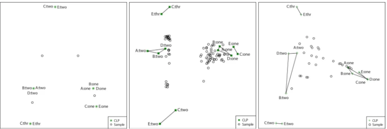
Figure 4.12 The sMCA biplot (observed subset) for the example data set (10% missing values with a MAR MDM with five variables and 1000 samples simulated from a uniform distribution). ... 86 Figure 4.13 Comparison of visualisation approaches for missing data compared to the complete MCA biplot. Left panel: complete MCA biplot (five variables and 1000 samples simulated from

(17)

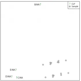
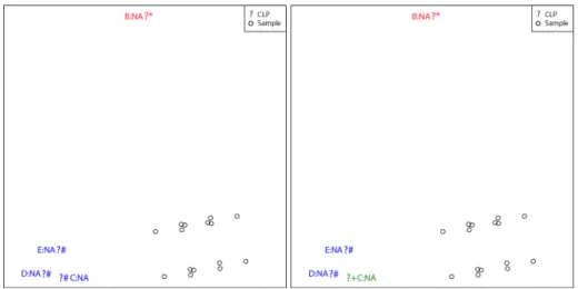
biplot (complete subset) (cf. Figure 4.12). Middle‐ and right panels: 10% missing values with a MAR MDM with five variables and 1000 samples simulated from a uniform distribution. ... 87 Figure 4.14 The CLP plot for the target configuration (CLPs from complete MCA) and testee (CLPs from GPAbin biplot) configuration before OPA. ... 88 Figure 4.15 The OPA steps. Left panel: Reflection and rotation of testee CLPs (GPAbin CLPs). Middle panel: Scaling of updated CLPs (reflected and rotated). Right panel: Target CLPs compared to updated testee CLPs. ... 89 Figure 4.16 Manually constructed convex hulls to mimic groupings in complete biplots. Left panel: complete MCA biplot (five variables and 100 samples simulated from a uniform distribution). Middle panel: GPAbin biplot. Right panel: sMCA biplot (complete subset). Middle‐ and right panels: 50% missing values with a MAR MDM with five variables and 100 samples simulated from a uniform distribution. ... 93 Figure 4.17 The sMCA biplot (missing subset) of the additional example data set (50% missing values with a MAR MDM with five variables and 100 samples simulated from a uniform distribution). ... 96 Figure 4.18 The pam clustering of CLPs in an sMCA biplot (missing subset) of the additional example data set (50% missing values with a MAR MDM with five variables and 100 samples simulated from a uniform distribution). Left panel: 2 → 0.6800. Right panel:

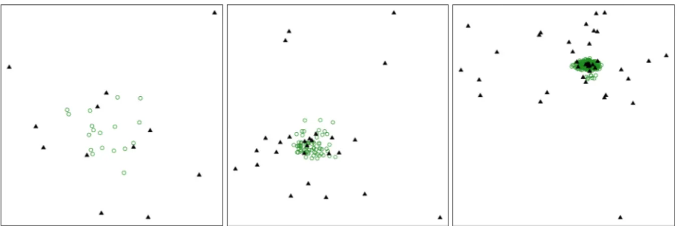
3 → 0.1848. ... 98 Figure 5.1 MCA biplots for Dirichlet simulations Left panel: 100, 5. Middle panel:

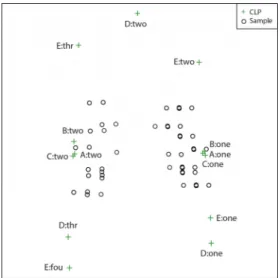
100, 10. Right panel: 3000, 15. Sample points are depicted by green open circles and CLPs by black triangles. ... 101 Figure 5.2 MCA biplots for uniform simulations. Left panel: 100, 5. Middle panel:

100, 10. Right panel: 3000, 15. Sample points are depicted by green open circles and CLPs by black triangles. ... 102 Figure 5.3 MCA biplots for normal simulations. Left panel: 100, 5. Middle panel:

100, 10. Right panel: 3000, 15. Sample points are depicted by green open circles and CLPs by black triangles. ... 102 Figure 5.4 MCA biplot with CLP labels of Figure 5.3 (left panel) ... 103 Figure 5.5 True percentage of missing values for Dirichlet simulations. Left panels: MAR 10% (mean missing values: 9.97%, minimum missing value percentage: 9.2%). Middle panels: MAR 30% (mean missing values: 29.4%, minimum missing value percentage: 20.1%). Right panels: MAR 50% (mean missing values: 38.8%, minimum missing value percentage: 20.1%). The simulations are sorted in the upper panels. ... 106 Figure 5.6 True percentage of missing values for uniform simulations. Left panels: MAR 10% (mean missing values: 9.96%, minimum missing value percentage: 9.3%). Middle panels: MAR 30% (mean missing values: 29.8%, minimum missing value percentage: 21.1%). Right panels: MAR 50% (mean missing values: 42.1%, minimum missing value percentage: 21.1%). The simulations are sorted in the upper panels. ... 107

(18)

Figure 5.7 True percentage of missing values for normal simulations. Left panels: MAR 10% (mean missing values: 9.96%, minimum missing value percentage: 9.2%). Middle panels: MAR 30% (mean missing values: 29.8%, minimum missing value percentage: 15.3%). Right panels: MAR 50% (mean missing values: 46.0%, minimum missing value percentage: 15.3%). The simulations are sorted in the upper panels. ... 108 Figure 6.1 Similarity percentages of all simulation scenarios for GPAbin, sMCA and RIMCA. ... 116 Figure 6.2 Density ridge plots to illustrate skewness of measures of comparison. A selection of simulation scenarios are illustrated. ... 127 Figure 6.3 AMB values per simulation scenario over 1000 repetitions (comparison in two dimensions). Left panel: Median AMB values. Right panel: Mean AMB values. ... 130 Figure 6.4 sMCA approach: 50% missing values with a MAR MDM for the three simulation distributions. ... 131 Figure 6.5 MB values per simulation scenario over 1000 repetitions (comparison in two dimensions). Left panel: Median MB values. Right panel: Mean MB values. ... 132 Figure 6.6 Scatterplots of the MB values for the sMCA method (MAR MDM). Left panels: 10% missing values. Middle vertical panels: 30% missing values. Right panels: 50% missing values. Upper panels: Dirichlet distribution. Middle horizontal panels: uniform distribution. Lower panel: normal distribution. ... 133 Figure 6.7 Scatterplots of the MB values for the sMCA method (MCAR MDM). Left panels: 10% missing values. Middle vertical panels: 30% missing values. Right panels: 50% missing values. Upper panels: Dirichlet distribution. Middle horizontal panels: uniform distribution. Lower panel: normal distribution. ... 134 Figure 6.8 RMSB values per simulation scenario over 1000 repetitions (comparison in two dimensions). Left panel: Median RMSB values. Right panel: Mean RMSB values. ... 135 Figure 6.9 PS values per simulation scenario over 1000 repetitions (comparison in two dimensions). Left panel: Median PS values. Right panel: Mean PS values. ... 137 Figure 6.10 Scatterplots of PS values for the GPAbin approach across all simulation scenarios. .... 140 Figure 6.11 Scatterplots of PS values for the RIMCA approach across all simulation scenarios. ... 141 Figure 6.12 Scatterplots of PS values for the sMCA approach across all simulation scenarios. ... 142 Figure 6.13 CC values per simulation scenario over 1000 repetitions (comparison in two dimensions). Left panel: Median CC values. Right panel: Mean CC values. ... 143 Figure 6.14 Scatterplots of normal distribution simulations: 50% missing values and MAR MDMs. Left panel: GPAbin. Middle panel: sMCA. Right panel: RIMCA. ... 144 Figure 6.15 Measures of comparison values per simulation scenario over 1000 repetitions (comparison in maximum dimensions). Left panel: Mean RMSB values. Right panel: Mean AMB values. ... 146 Figure 6.16 Mean PS values per simulation scenario over 1000 repetitions (comparison in maximum dimensions). ... 147

(19)

Figure 7.1 Measures of comparison values per simulation scenario over 1000 repetitions (comparison in two dimensions). Left panel: Mean AMB values. Right panel: Mean RMSB values. ... 152 Figure 7.2 Kernel density estimates of AMB values for prediction methods (MCN 30% missing values). ... 153 Figure 7.3 Kernel density estimates of AMB values for prediction methods (MC 50% missing values).

... 154 Figure 7.4 Measures of fit values per simulation scenario over 1000 repetitions (comparison in two dimensions). Left panel: Mean PS values. Right panel: Mean CC values. ... 156 Figure 7.5 PS values: Dirichlet distribution (GPAbin prediction, Majority rule prediction and GPAbin)

... 158 Figure 7.6 PS values: Uniform distribution (GPAbin prediction, Majority rule prediction and GPAbin)

... 159 Figure 7.7 PS values: Normal distribution (GPAbin prediction, Majority rule prediction and GPAbin)

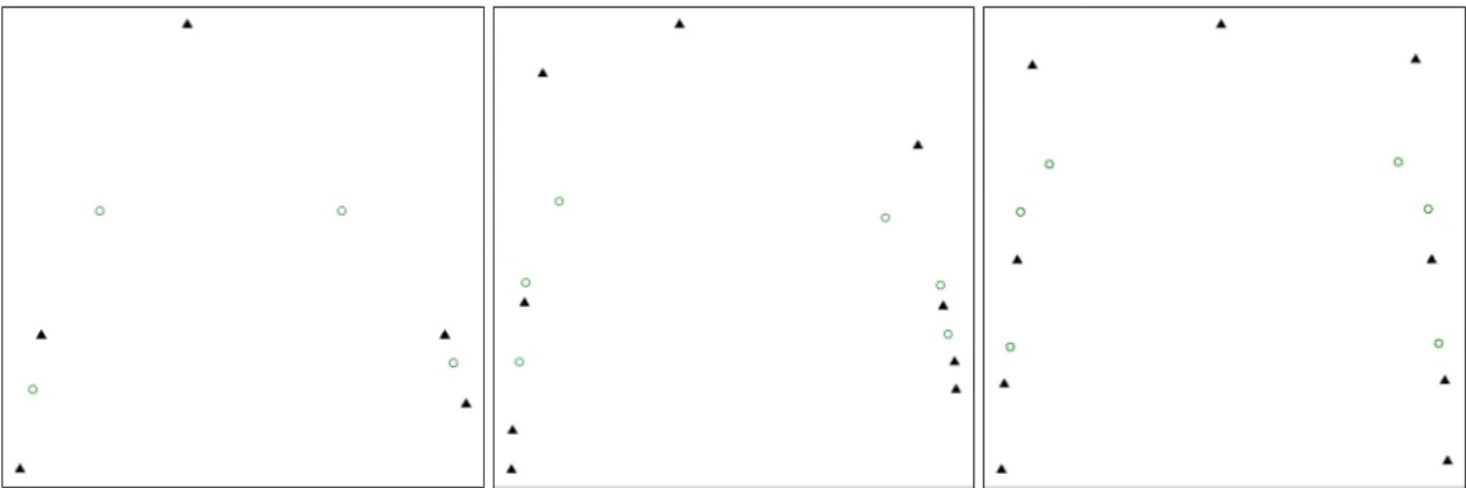
... 160 Figure 8.1 sMCA biplots for the missing subsets of a selected repetition ( 100, 5). Sample points are depicted by green open circles and CLPs by black triangles. Take note that the number of CLPs of the MAR simulations is one less than the number of MCAR CLPs (cf. 5.4). ... 167 Figure 8.2 sMCA biplots for the missing subsets of a selected repetition ( 100, 10). Sample points are depicted by green open circles and CLPs by black triangles. Take note that the number of CLPs of the MAR simulations is one less than the number of MCAR CLPs (cf. 5.4). ... 168 Figure 8.3 sMCA biplots for the missing subsets of a selected repetition ( 100, 15). Sample points are depicted by green open circles and CLPs by black triangles. Take note that the number of CLPs of the MAR simulations is one less than the number of MCAR CLPs (cf. 5.4). ... 169 Figure 8.4 sMCA biplots for the missing subsets of a selected repetition ( 1000, 5). Sample points are depicted by green open circles and CLPs by black triangles. Take note that the number of CLPs of the MAR simulations is one less than the number of MCAR CLPs (cf. 5.4). ... 170 Figure 8.5 sMCA biplots for the missing subsets of a selected repetition ( 1000, 10). Sample points are depicted by green open circles and CLPs by black triangles. Take note that the number of CLPs of the MAR simulations is one less than the number of MCAR CLPs (cf. 5.4). ... 171 Figure 8.6 sMCA biplots for the missing subsets of a selected repetition ( 1000, 15). Sample points are depicted by green open circles and CLPs by black triangles. Take note that the number of CLPs of the MAR simulations is one less than the number of MCAR CLPs (cf. 5.4). ... 172 Figure 8.7 sMCA biplots for the missing subsets of a selected repetition ( 3000, 5). Sample

(20)

number of CLPs of the MAR simulations is one less than the number of MCAR CLPs (cf. 5.4). ... 173 Figure 8.8 sMCA biplots for the missing subsets of a selected repetition ( 3000, 10). Sample points are depicted by green open circles and CLPs by black triangles. Take note that the number of CLPs of the MAR simulations is one less than the number of MCAR CLPs (cf. 5.4). ... 174 Figure 8.9 sMCA biplots for the missing subsets of a selected repetition ( 3000, 15). Sample points are depicted by green open circles and CLPs by black triangles. Take note that the number of CLPs of the MAR simulations is one less than the number of MCAR CLPs (cf. 5.4). ... 175 Figure 8.10 Silhouette coefficients of the Dirichlet distribution (10% missingness). Upper panels: MAR MDM. Lower panels: MCAR MDM. Left panels: scatterplots. Right panels: stacked bar plots. ... 177 Figure 8.11 Silhouette coefficients of the uniform distribution (10% missingness). Upper panels: MAR MDM. Lower panels: MCAR MDM. Left panels: scatterplots. Right panels: stacked bar plots. ... 180 Figure 8.12 Silhouette coefficients of the normal distribution (10% missingness). Upper panels: MAR MDM. Lower panels: MCAR MDM. Left panels: scatterplots. Right panels: stacked bar plots. ... 182 Figure 8.13 Silhouette coefficients of the Dirichlet distribution (30% missingness). Upper panels: MAR MDM. Lower panels: MCAR MDM. Left panels: scatterplots. Right panels: stacked bar plots. ... 184 Figure 8.14 Silhouette coefficients of the uniform distribution (30% missingness). Upper panels: MAR MDM. Lower panels: MCAR MDM. Left panels: scatterplots. Right panels: stacked bar plots. ... 185 Figure 8.15 Silhouette coefficients of the normal distribution (30% missingness). Upper panels: MAR MDM. Lower panels: MCAR MDM. Left panels: scatterplots. Right panels: stacked bar plots. ... 186 Figure 8.16 Silhouette coefficients of the Dirichlet distribution (50% missingness). Upper panels: MAR MDM. Lower panels: MCAR MDM. Left panels: scatterplots. Right panels: stacked bar plots. ... 188 Figure 8.17 Silhouette coefficients of the uniform distribution (50% missingness). Upper panels: MAR MDM. Lower panels: MCAR MDM. Left panels: scatterplots. Right panels: stacked bar plots. ... 189 Figure 8.18 Silhouette coefficients of the normal distribution (50% missingness). Upper panels: MAR MDM. Lower panels: MCAR MDM. Left panels: scatterplots. Right panels: stacked bar plots. ... 190 Figure 8.19 Heat map of the percentage of silhouette coefficients above 0.5 for 30% missingness.

(21)

Figure 8.21 Heat map of the percentage of silhouette coefficients above 0.6. ... 195 Figure 9.1 Bar graphs of each variable in the adapted survey: 1 – agree, 2 – neutral, 3 – disagree, NA – missing ... 202 Figure 9.2 sMCA biplot: missing subset of real data application. Left panel: standard sMCA biplot display. Right panel: sMCA biplot with samples colour coded according to educational level and represented as convex hulls. ... 203 Figure 9.3 Illustrating allocated clusters for the sMCA biplot (missing subset) of the real data application. Left panel: 2 → 0.7832. Middle panel: 3 → 0.5016. Right panel: 4 → 0.5805. ... 204 Figure 9.4 Illustration of CLPs before and after GPA for ten MIs. Each panel represents the CLPs for a particular MI for the real data application. ... 206 Figure 9.5 Superimposed transformed CLPs from Figure 9.4 for the real data application. ... 207 Figure 9.6 Left panel: Convex hulls of superimposed CLPs after GPA. Right panel: Colour coded convex hulls with increasing colour intensity according to the percentage of missing values ... 208 Figure 9.7 Left panel: GPAbin biplot. Right panel: CLP descriptions of GPAbin biplot. ... 208 Figure 9.8 Left panel: sMCA biplot. Right panel: CLP descriptions of sMCA biplot. ... 209 Figure 9.9 Colour coded CLPs according to the response level. Left panel: GPAbin biplot. Right panel: sMCA biplot. ... 210 Figure 9.10 GPAbin biplots with convex hulls for sample separation based on demographic information. Top panels: Gender (left), Region (middle) and Marital status (right). Lower panels: Education (left) and Age (right). ... 211 Figure 9.11 sMCA biplots with convex hulls for sample separation based on demographic information. Top panels: Gender (left), Region (middle) and Marital status (right). Lower panels: Education (left) and Age (right) ... 212

(22)

List of Tables

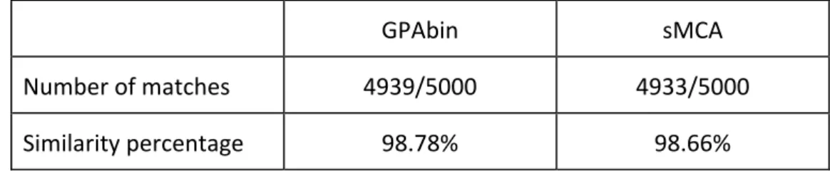
Table 2.1 Toy data set ... 13 Table 3.1 Toy data set with missing values ... 44 Table 3.2 Adapted toy data set with missing values ... 48 Table 4.1 Measures of comparison for the GPAbin CLPs of the example data set (10% missing values with a MAR MDM with five variables and 1000 samples simulated from a uniform distribution) compared to the CLPs of the complete MCA biplot (five variables and 1000 samples simulated from a uniform distribution). ... 92 Table 4.2 Similarity percentages obtained from GPAbin and sMCA when compared to the complete MCA biplot in two dimensions, respectively. Example data set: 10% missing values with a MAR MDM with five variables and 1000 samples simulated from a uniform distribution ... 95 Table 5.1 Allocating CLs from continuous values ... 101 Table 5.2 The number of cores used for the computations of uniform distribution simulations with 50% missing values inserted with an MCAR MDM... 111 Table 5.3 The RAM (in GB) used for the computations of uniform distribution simulations with 50% missing values inserted with an MCAR MDM. ... 112 Table 5.4 The walltime (in minutes) used for the computations of uniform distribution simulations with 50% missing values inserted with an MCAR MDM. ... 112 Table 6.1 Abbreviations for simulation distributions and MDMs ... 114 Table 6.2 Coefficients of variation of similarity percentages (GPAbin, sMCA and RIMCA) for all simulation scenarios. Values above 3% are indicated in bold font. ... 118 Table 6.3 Similarity percentages of simulation scenarios with 30% missing values with a coefficient of variation greater than 3% between approaches (bold values of Table 6.2). ... 119 Table 6.4 Similarity percentages of simulation scenarios with 50% missing values with a coefficient of variation greater than 3% between approaches (bold values of Table 6.2). ... 120 Table 6.5 Similarity percentages below 75% for simulation scenarios with 10% missing values. Investigating the percentages of Figure 6.1. ... 121 Table 6.6 Similarity percentages below 75% for simulation scenarios with 30% missing values. Investigating the percentages of Figure 6.1. ... 122 Table 6.7 Similarity percentages below 75% for simulation scenarios with 50% missing values. Investigating the percentages of Figure 6.1. ... 123 Table 6.8 Ranges for measures of comparison: missing data approaches ... 128 Table 6.9 Top 10% ranges for measures of comparison: missing data approaches ... 129 Table 7.1 Ranges for measures of comparison: prediction methods. ... 150 Table 7.2 Top 10% ranges for measures of comparison: prediction methods ... 150

(23)

Table 9.2 Variable information for demographic questions of ISSP 1994. ... 201 Table 9.3 Measures of comparison: GPAbin and sMCA real application ... 213

(24)

List of Abbreviations

Acronyms

CART Classification and regression trees

MAR Missing at random

OPA Orthogonal Procrustes analysis

MIMCA Multiple imputation using multiple correspondence analysis

pam partitioning around medoids

RAM Random‐access memory

RIMCA Regularised iterative multiple correspondence analysis

Initialisms

AMB Absolute mean bias

CA Correspondence analysis

CC Congruence coefficient

CL Category level

CLs Category levels

CLP Category level point

CLPs Category level points

EM Expectation‐Maximisation

FCS Fully conditional specification

GB Gigabyte

GPA Generalised orthogonal Procrustes analysis

GSVD Generalised singular value decomposition

(25)

MA Data simulated from a uniform distribution with a missing at random missing

data mechanism

MAD Data simulated from a Dirichlet distribution with a missing at random missing

data mechanism

MAN Data simulated from a normal distribution with a missing at random missing

data mechanism

MB Mean bias

MC Data simulated from a uniform distribution with a missing completely at

random missing data mechanism

MCA Multiple Correspondence analysis

MCD Data simulated from a Dirichlet distribution with a missing completely at

MCN Data simulated from a normal distribution with a missing completely at

MDM Missing data mechanism

MDS Multidimensional scaling

MI Multiple imputation

MIs Multiple imputations

MSEP Mean square error of prediction

PS Procrustes Statistic

RMSB Root mean squared bias

sCA Subset correspondence analysis

SI Single imputation

sMCA Subset multiple correspondence analysis

SVD Singular value decomposition

(26)

Combination of acronyms and intialisms

GPAbin Generalised Procrustes analysis and Rubin’s rules

‘GPA’ – initialism and ‘bin’ – acronym

MCAR Missing completely at random

‘M’ – initialism and ‘CAR’ – acronym

MNAR Missing not at random

‘M’ – initialism and ‘NAR’ – acronym

(27)

Chapter 1 Rationale

1.1 Introduction

Missing data have become a prevalent problem which is in a sense inseparable from data

collection. Over the past decades, proper missing data handling techniques have been

developed and applied for the imputation of missing data sets (Van Buuren, 2012). Various

imputation techniques are available to substitute missing observations with plausible

response values. Single imputation (SI) is the substitution of a single plausible response for

each missing observation, which is easy to apply but generally results in biased estimation, as

the standard errors are underestimated (Rubin, 1987). Multiple imputation (MI) is the

preferred method that generates several plausible values for each missing value until a

predetermined number of data sets are imputed. This results in unbiased representation of

the missing observations, as it provides a distribution of plausible responses to capture the

uncertainty involved in the task of imputation. Standard analyses for complete data are then

applied to the multiple data sets and the estimates of interest can be combined to formulate

a final inferential statement (Rubin, 1987; Schafer, 1997; Van Buuren, 2012). The study of MI

might be considered somewhat controversial, because the imputations are not applied with

the aim of obtaining a final completed data set, but rather to preserve the population

variation and, most importantly, the relationships between variables (Wayman, 2003).

The importance of both SI and MI is acknowledged and the development of MI should not be

regarded as a replacement for SI, but rather an improvement to handle missing data in more

complex scenarios. In some cases, however, the aim might be to only obtain one completed

data set to be used by field specialists, and therefore SI is still relevant. Nevertheless, from an

analyst’s perspective, there is much to be gained from the unbiased estimation of the

variation when using MI.

The study of data imputation remains a growing topic of interest, but visualisations for

missing data and completed data have not yet been placed on the foreground of statistical

analysis (Eaton, Plaisant & Drizd, 2005; Fernstad, 2019; Templ, Alfons & Filzmoser, 2012).

(28)

could lead to biased inference. Therefore, this study focusses on the development of

appropriate exploratory techniques for multivariate categorical missing data and multiple

imputed data sets. In a recent review on missing data protocols the remark was made that

“new research on diagnostics and visualisation may inform analyses with missing values”

(Josse & Reiter, 2018: 141). This is motivation that the developments in this research will

address current missing data issues and contribute to the science of handling missing data.

In this study, three core methodologies will be extended and combined, namely multivariate

categorical data analysis, missing data analysis and biplot visualisation.

1.2 Data

Only nominal scaled multivariate categorical data are considered in this study. Consider a set

of individuals where measurements are made for each individual (referred to as a sample) on

a set of categorical questions (referred to as variables). A nominal scaled measurement on a

categorical variable can only be one of a finite unordered number of qualities, for example

hair colour: red, blonde or brunette. There is no specific order of importance of the qualitative

response options (Agresti, 2007). These qualities are referred to as the category levels (CLs)

of a categorical variable. Typically, the categorical variables are represented as the columns

of a matrix and the samples as its rows. The proposed methodology will be applied to a variety

of simulated data scenarios (cf. Chapter 5) consisting of combinations from different

distributions, dimensions, percentages of missing values and missing data mechanisms

(MDMs). The results obtained from a real application are presented in Chapter 9.

1.3 Visualisations

Multiple correspondence analysis (MCA) is a multivariate categorical technique that enables

the simultaneous exploration of samples and their different qualitative responses measured

for all the categorical variables. The focus of MCA is to obtain an understanding of how the

samples are associated based on their responses to variables. Samples are regarded as similar

if they have a majority of the same responses to variables (i.e. CLs). The main interest is the

(29)

Husson, 2012). Even though quantities of association can be calculated, it is only truly

understood when it is visualised (Beh & Lombardo, 2014). Biplots are constructed from MCA

solutions for visual inspections of the categorical data. Biplots are regarded as multivariate

scatterplots approximated in lower dimension, in which multiple variables and samples are

represented in a single configuration. The biplot display enables the immediate grasp of

response patterns and associations between samples based on the distances between

coordinates in the display space. Points in close proximity are regarded as being highly

associated and reflect individuals with similar response profiles. The biplot consists of sample

coordinates, one for each sample, and category level points (CLPs), one for each CL of a

particular variable. Each sample is positioned such that the response CL will be in close

proximity in the approximated two‐dimensional space. Biplots are typically displayed in two

dimensions. However, the prefix, ‘bi’, does not refer to the dimension of the display space,

but refers to the simultaneous representation of both samples and CLPs (Gower & Hand,

1996; Husson et al., 2011). The term ‘configurations’ will refer to MCA biplots throughout the

dissertation.

Computational power and sufficient software have greatly influenced the use and popularity

of exploratory analysis (Unwin, Chen & Härdle, 2008). Because multiple visualisations can be

produced within seconds, the adequate interpretation of the resulting large number of

visualisations can become overwhelming. This is an additional branch of data science and big

data.

There is a need for methodology to provide unbiased combined visual representations of

different variations of the same data. This will allow the evaluation of the subtle differences

between multiple visualisations that could be lost when examining a large number of

individual graphical displays.

1.4 Aim and study objectives

The aim of this research is to develop unbiased visualisations for multivariate categorical

(30)

 Obtaining an unbiased single visualisation after MI

 Determining the applicability of visualisations without prior imputation

 Obtaining a single completed categorical data set using predictions from visualisations

 Identifying the MDM using visualisation.

The four study objectives can be achieved by formulating novel methodologies by unifying

the concepts of categorical data analysis, missing data analysis and data visualisation.

Simulated data play a vital role in the evaluation of missing data techniques. Simulation

enables the comparison of inferences obtained from complete data and completed data of

the same initial simulated data set. Therefore, an extensive simulation study is called for to

evaluate the methodology of the four study objectives when applied to various missing data

scenarios.

1.4.1 The GPAbin objective

The first objective is to optimally combine the configurations obtained from MIs of

multivariate categorical data with missing data entries into a single biplot display.

A single visualisation for MIs can enhance the exploratory analysis of incomplete data. The

visualisation of combined MIs has not yet been explored to aid in the understanding of the

variation between the imputations. Visualisations of MIs have been projected as

supplementary points onto a reference framework for continuous data using principal

component analysis (PCA) by Josse and Husson (2012). Procrustes analysis was used to align

the imputation visualisations to a reference set individually in order to evaluate the variation

between the imputations. Apart from using confidence ellipses to illustrate the uncertainty

between MIs, no concrete measure was used to evaluate the success of the projection

methods.

Since MCA is a suitable technique to evaluate the relationships between variables and

consistencies among samples for multivariate categorical data, MCA biplots are a fitting

choice for the visualisation (Blasius & Thiessen, 2012; Greenacre, 2010; Josse & Husson,

(31)

address the methodology to achieve this study objective, a few known techniques have to be

considered. Two configurations with the same dimensions (number of samples and variables)

can be compared using orthogonal Procrustes analysis (OPA). One configuration is set as a

target to which the testee configuration is transformed using admissible transformations

(Borg & Groenen, 2005; Gower & Dijksterhuis, 2004; Ten Berge, 1977). As we are interested

in the visualisation of MIs, a technique that enables the comparison of more than two

configurations is required. Generalised orthogonal Procrustes analysis (GPA) allows the

comparison of multiple configurations to determine the associations or dissimilarities among

multiple configurations when compared to a chosen target configuration (Gower &

Dijksterhuis, 2004). After the application of GPA, the multiple configurations are optimally

aligned, which improves the visual interpretation thereof. The visualisation of multiple

plausible final data sets allows the interpretation of MIs from a new perspective, unlocking

additional information only available utilising visual aids. The differences between each

imputation can be explored to determine the robustness of the chosen imputation technique.

As MI successfully incorporates variation and uncertainty, it is to be expected that there will

be differences between the MI MCA solutions. However, if substantial differences are

observed between MI visualisations, the validity of the imputation technique should be

investigated for the particular data and missing data problem.

Even though GPA eases visual inspection by aligning the configurations, inspecting a large

number of separate visualisations (one figure for each imputation) could become tedious and

as the number of MIs increases, it becomes impossible to draw accurate inferences from the

separate configurations. A single combined display could allow the instantaneous

interpretations of associations between variables and samples, which would not have been

possible with separate configurations for each imputation. Therefore, a centroid

configuration containing the mean coordinates of the optimally aligned configurations is

proposed to represent the visualisation of the MIs. The centroid configuration resonates with

the application of Rubin’s rules (Rubin, 1987) to combine estimates obtained from MIs.

Now, the aim is not to obtain a final inferential statement, but rather a final descriptive

visualisation for the exploratory analysis as opposed to a confirmatory one. The combined

visualisation technique is defined by the term, ‘GPAbin’, which pays tribute to the

(32)

The application of GPA has shown to be successful in obtaining a final loading matrix from

PCA loadings of MIs (Van Ginkel & Kroonenberg, 2014) and has also been proposed to visually

evaluate the between‐imputation variation of MIs in PCA (Josse & Husson, 2012). However,

GPA has not yet been explored to aid as a combination technique for MI visualisations in

incomplete categorical data analysis, which confirms the novelty of this development. All final

configurations are compared to the MCA biplot of the simulated complete data using

measures of comparison within the Procrustes framework. An SI technique is also applied in

order to determine the success of constructing a GPAbin configuration in comparison to a

single configuration from single imputed data.

1.4.2 The subset multiple correspondence analysis objective

The second objective is to determine whether non‐imputed data can be successfully

visualised to preserve the associations between samples and their responses.

The visualisation of incomplete multivariate data without prior imputation is an intriguing

possibility for the non‐technical practitioner. Subset correspondence analysis (sCA) has been

used to explore incomplete categorical data consisting of two‐way contingency tables

(Greenacre, 2017; Hendry, North, Zewotir & Naidoo, 2014). The complete correspondence

analysis (CA) can be restricted using a chosen subset of a data matrix while maintaining the

original column and row masses for the calculation of the distances. Therefore, the total

variation (inertia) is partitioned into components associated with the various subsets and no

interpretable information is lost. This idea is extended to MCA, referred to as subset MCA

(sMCA). The data matrix of a multivariate categorical data set is commonly coded as an

indicator matrix of zeros and ones. The columns of the indicator matrix represent the CLs and

the rows correspond to the samples. A particular response will be represented by a one in the

column corresponding to the chosen CL and zero elsewhere. In the case of multi‐way

contingency tables, sMCA can be applied for the visualisation of the missing observations by

recoding the indicator matrix. New CLs are created for the missing responses, which is an

active handling approach to missing data (cf. 3.4.2.2). The missing CLs can then be separated

from the observed CLs, which allows a focused analysis on either missing or observed subsets.

(33)

1.4.3 The prediction objective

The third study objective advances naturally from the MI‐ and GPAbin visualisations. Even

though MI techniques focus on overall inference obtained from multiple plausible completed

data sets, it is an intriguing idea to determine whether a single data set can be successfully

predicted. The distances between coordinates in the visualisations of MIs and the GPAbin

procedure (cf. 1.4.1) can be used to predict possible responses. Two approaches to predict a

final categorical data set are proposed. The distances in the full space (all available

dimensions) between the sample coordinates and CLPs are used to identify the CLP in closest

proximity to a sample coordinate for each variable. The use of distances to predict a response

is similar to nearest‐neighbour imputation (Biemer & Lyberg, 2003; Ohmann, Gregory,

Henderson & Roberts, 2011).

As the focus of this research is visualisation, MCA biplots are also constructed for the

predicted data sets. The success of the prediction methods is determined by comparing the

visualisations of the predicted data sets to the visualisations of the simulated complete data

sets.

1.4.4 The missing data mechanism objective

The fourth study objective is to identify the MDM using the missing CLs obtained from the

sMCA procedure discussed in the second study objective (cf. 1.4.2). It is crucial to understand

the cause of missingness before selecting a missing data handling technique (Buhi, Goodson

& Neilands, 2008; Kowarik & Templ, 2016). Exploring visualisations of missing values expose

structures and patterns that are not perceptible in a data table (Templ et al., 2012). The

occurrence of missing values can be explained as the result of a random process referred to

as the MDM (Van Buuren, 2012). Three mechanisms are defined: missing at random (MAR),

missing completely at random (MCAR) and missing not at random (MNAR). Non‐responses in

categorical data sets commonly occur in questionnaires, which could be due to the deliberate

omission of sensitive questions that in some cases are related to answered questions in the

questionnaire. This is an example of observations that are classified as being MAR, as the

missing values are dependent on the observed values in the data set. Respondents may also

(34)

as missing observations are independent of observed and missing observations (García‐

Laencina, Sancho‐Gómez & Figueiras‐Vidal, 2010). Missing observations that are unobserved

due to the MNAR mechanism are dependent on observations that are not captured by the

questionnaire, therefore dependent on other missing values. This occurs when questions in

the questionnaire could be related to information that is not captured or considered by the

particular questionnaire (Schafer & Graham, 2002). There are three assumptions that have to

be satisfied for a proper MI procedure (cf. 3.4.4.2). Only the first assumption is considered for

this study objective, which is the uncertainty of identifying the MDM before selecting an

imputation procedure (Rubin, 2003). Apart from the three MDM descriptions, there are two

main classifications: ignorable and non‐ignorable non‐response. The MNAR MDM is

categorised as non‐ignorable (informative), as the missing data entries are dependent on

information that is not available. This means that standard statistical analyses will not capture

the uncertainty of these particular missing values (Buhi et al., 2008). However, the MAR MDM

and MCAR MDM are in some way related to the missing or observed observations and are

regarded as ignorable (non‐informative) missingness, which allows the application of

standard missing data techniques (Buhi et al., 2008; Schafer & Olsen, 1998).

Only the ignorable MDMs will be explored in this objective. The missing CLPs from the sMCA

solution are configured in a biplot. The dependency of the missing data entries on the

observed entries in the MAR MDM is expected to result in distinguishable patterns and

clusters / groupings. It is expected that no particular pattern will be identified in the sMCA

biplot of the missing CLPs of a MCAR MDM, as all observations have the same probability of

being missing.

The partitioning around medoids (pam) clustering technique (Maechler, Rousseeuw, Struyf,

Hubert & Hornik, 2017) will be used to determine the number of clusters that can be

successfully separated in the incomplete sMCA biplots.

Biplot methodology for analysing and evaluating missing multivariate nominal scaled data

evaluating

missing

multivariate

nominal

scaled

data

Submitted

by

JOHANÉ

NIENKEMPER

‐

SWANEPOEL

Dissertation

presented

for

the

degree

of

Doctor

of

Philosophy

in

the

Department

of

Statistics

and

Actuarial

Science

in

the

Faculty

of

Economic

and

Management

Sciences

at

Stellenbosch

University.

Supervisor:

Professor

NJ

le

Roux

Co

‐

supervisor:

Professor

S

Gardner

‐

Lubbe

Declaration

Abstract

Opsomming

Acknowledgements

Table of Contents

List of Figures

List of Tables

List of Abbreviations

Chapter 1

Rationale