Title
The parameter sensitivity of random forests.
Permalink
https://escholarship.org/uc/item/3pm875xd
Journal
BMC bioinformatics, 17(1)
ISSN
1471-2105
Authors
Huang, Barbara FF
Boutros, Paul C
Publication Date
2016-09-01
DOI
10.1186/s12859-016-1228-x
Peer reviewed
eScholarship.org
Powered by the California Digital Library
M E T H O D O L O G Y A R T I C L E
Open Access
The parameter sensitivity of random forests
Barbara F.F. Huang
1and Paul C. Boutros
1,2,3,4*Abstract
Background:The Random Forest (RF) algorithm for supervised machine learning is an ensemble learning method widely used in science and many other fields. Its popularity has been increasing, but relatively few studies address the parameter selection process: a critical step in model fitting. Due to numerous assertions regarding the performance reliability of the default parameters, many RF models are fit using these values. However there has not yet been a thorough examination of the parameter-sensitivity of RFs in computational genomic studies. We address this gap here.
Results:We examined the effects of parameter selection on classification performance using the RF machine learning algorithm on two biological datasets with distinctp/nratios: sequencing summary statistics (lowp/n) and microarray-derived data (highp/n). Here,p,refers to the number of variables and,n, the number of samples. Our findings demonstrate that parameterization is highly correlated with prediction accuracy and variable importance measures (VIMs). Further, we demonstrate that different parameters are critical in tuning different datasets, and that parameter-optimization significantly enhances upon the default parameters.
Conclusions:Parameter performance demonstrated wide variability on both low and highp/ndata. Therefore, there is significant benefit to be gained by model tuning RFs away from their default parameter settings. Keywords:Machine-learning, Random forest, Parameterization, Computational biology, Ensemble methods, Optimization, Microarray, SeqControl
Abbreviations:AUC, Area under the receiver operating characteristic curve; DFCI, Dana-Farber Cancer Institute; HLM, Moffitt Cancer Center; HPCI, High performance computing interface; ICGC, International Cancer Genome Consortium; ML, Machine learning; MSKCC, Memorial Sloan-Kettering Cancer Center; NSCLC, Non-small cell lung cancer; OOB, Out-of-bag; RF, Random forest; RMSE, Root mean squared error; UM, University of Michigan Cancer Center; VIM, Variable importance measure
Background
Machine learning (ML) techniques are widely used in the analysis of high-throughput data to answer a broad range of biological questions. Applications in the field of medicine have transformed our understanding of complex genomic interactions and measurements [1]. ML has been successfully applied to biological disci-plines including proteomics [2, 3], drug development [4, 5], DNA sequence analysis [6–8], cancer classification [9–13], clinical decision making [14, 15], and biomarker discovery [16, 17]. The versatility of ML algorithms to
broad ranges of data and applications offers powerful, yet generalizable solutions to biological questions.
Recently, the random forest (RF) algorithm [18] for ML has achieved broad popularity. RF is a form of ensemble learning and possesses several characteristics that impart versatility. It can be applied to two-class or multi-class prediction problems, model interactions among variables, can take on a mixture of categorical and continuous variables, provides variable importance measures (VIMs), and has good predictive performance even for data with more variables (p) than samples (n; i.e.p> >n); potentially involving highly noisy and signifi-cantly correlated variables [19, 20]. Due to their non-parametric nature, RFs are fairly robust with relatively straightforward applications for inexperienced users [21, 22]. Consequently, this algorithm has expanded to a framework of models [23].
* Correspondence:[email protected]
1Informatics and Bio-computing Program, Ontario Institute for Cancer Research, Toronto, Canada
2Department of Medical Biophysics, University of Toronto, Toronto, Canada Full list of author information is available at the end of the article
© 2016 The Author(s).Open AccessThis article is distributed under the terms of the Creative Commons Attribution 4.0 International License (http://creativecommons.org/licenses/by/4.0/), which permits unrestricted use, distribution, and reproduction in any medium, provided you give appropriate credit to the original author(s) and the source, provide a link to the Creative Commons license, and indicate if changes were made. The Creative Commons Public Domain Dedication waiver (http://creativecommons.org/publicdomain/zero/1.0/) applies to the data made available in this article, unless otherwise stated.
To train a random forest model, a bootstrap [24] sam-ple is drawn, with the number of samsam-ples specified by the parameter sampsize [25]. By default, the bootstrap sample has the same number of samples as the original data: some samples are represented multiple times, whereas others are absent, leading to approximately 37 % of samples being absent in any given tree. These are referred to as the out-of-bag (OOB) samples [26]. Independent of thesampsizesetting, after each sample is drawn, a decision tree is created. In the most commonly-used implementation, fully-grown or un-pruned decision trees are created [18]. The number of trees is denoted by the parameterntree[21]. This
collec-tion of models is known as bootstrap aggregacollec-tion or bagging [27] and is commonly applied to high-variance and low-bias learners such as trees [28, 29]. Since indi-vidual trees are more prone to over-fitting than a collec-tion of trees, an ensemble method has a significant advantage [27, 29]; however, this is limited by the correl-ation between the trees and can be mitigated by choos-ing a number of randomly selected input variables at each split of the tree. The number of random variables used at each split is denoted by the parameter mtry. Of
this subset of randomly selected variables, the one that forms the best split is selected [25, 30]. The best split is selected on the basis of a specific objective function, most typically maximization of the Gini coefficient or total gain in purity. This produces the most homoge-neous groups and lowest OOB error [21]. Several empir-ical studies have shown the benefit of aggregating multiple trees to create a strong learner whereas, inde-pendently they would be considered unstable with lower classification accuracy [27, 31–34].
Machine learning algorithms frequently require esti-mation of model parameters and hyper-parameters, commonly through grid-searching [35]. Surprisingly, though, this is not common practice in the literature for RFs, where default values are often used as it is widely believed that this method is parameter-insensitive, or at least robust to changes from default parameter settings [36–38]. To test this assumption, we performed an exhaustive analysis of the parameter-sensitivity of RFs in two large, representative bioinformatics datasets. We show that our top performing tuned models were able to achieve greater prediction accuracies than the default models for both datasets and that the performance of the default parameterization is inconsistent. This empha-sizes the value of per-dataset tuning of RF models. Results
Experimental design
To evaluate the sensitivity of RF models to
parameterization, we selected two datasets representative of those commonly used in computational biology. The
first studies quality-control metrics in next-generation sequencing [6] and comprises 15 features (sequencing quality metrics) with 720 training samples and 576 validation samples, and thus reflects lowp/nratio studies. Each sample was classified as“good library”or“bad library” based on information external to the 15 features, and our models aimed to predict this binary response variable.
The second dataset reflected high p/n studies and comprises three categorical clinical variables and 12,135 continuous mRNA abundances for Non-Small Cell Lung Cancer (NSCLC) patients [13]. We trained models to predict patient outcome, “no death” or “death”. There were 255 samples in the training cohort.
For both datasets, we performed two model-fitting steps (Fig. 1). First, we selected a broad and comprehen-sive range of parameters (Additional file 1), and trained a RF classification model for each combination, includ-ing the default parameters. Models were trained on the training dataset and validated on a fully independent dataset. Performance was scored using the Area Under the Receiver Operating Characteristic Curve (AUC) [38]. Second, we fit an RF regression model using the data from the previous step: parameters were set as the co-variates and AUC as the response. This allows us to characterize the association between prediction accuracy and parameterization. We randomly sampled 2/3 of parameter sets for training and reserved the remainder for validation. We aimed to predict the withheld AUC scores and assessed performance using Spearman's Rank Correlation Coefficient (ρ) and Lin's Concordance Correlation Coefficient (ρc).
Prediction accuracy is a strong function of parameterization in lowp/nstudies
We first evaluated the parameter sensitivity of RF pre-diction accuracy in the low p/n dataset. We created 1,500 different sets of parameters and evaluated the per-formance of each. Most models succeeded at this task (Fig. 2), with a median AUC of 0.893 and 96 % of models exceeding 0.80 AUC. However, the performance varied dramatically, with a range of 0.6113–0.9996, suggesting that some parameterizations greatly improve or hinder prediction accuracy. The default parameterization (ntree
= 500, mtry= 3, sampsize= 720 with replacement)
per-formed well, with an AUC of 0.9726 and ranked in the top 12 % of all models (174/1,500; Additional file 2). This clearly demonstrates that the default settings are reasonable, but not optimal.
We asked if models were consistently struggling with the same samples. We looked for samples in the validation dataset where at least 50 % of models trained with different parameter sets made incorrect predictions. In total 73/576 (12.7 %) of validation samples were diffi-cult to classify. These were strongly asymmetrically
distributed between the classes with 72/432 (17 %)“good library” validation samples difficult to classify relative to only 1/144 (1 %)“bad library”validation samples (p= 1.27 × 10⁻⁶; proportion-test). Interestingly though, the global error rate was not dramatically different between these two groups (20 % for “good library” vs. 14 % for“bad library” samples).
Parameterization was strongly correlated to AUC score (Fig. 2) in this dataset, but tightly focused on specific parameters. The number of variables sampled per node (mtry) was strongly negatively correlated with AUC
(ρmtry= -0.895) andmtry≤3 resulted in higher
classifica-tion accuracy (mean AUC formtry≤3 = 0.97; mean AUC
for mtry> 3 = 0.88; Welch Two Sample t-test). In
contrast, models were relatively robust to changes in the
ntree and sampsize parameters (ρntree= 0.053 and ρ samp-size= 0.096; Spearman'sρ).
To further explore the relationship between parameterization and performance, we univariately compared performance within each parameter (Additional file 1), with Benjamini-Hochberg adjustment for multiple-testing [39]. While sampsize values did not differ significantly from each other, however, ntree of 10 had
significantly lower AUCs (q< 0.05) than other setting (Additional files 3, 4 and 5). Similarly, as noted above there was a near-linear relationship between increasing mtry and decreasing AUC in the validation cohort
(Additional file 6). These findings illustrated the strong in-fluence of parameter selection on classification accuracy, and that both linear and threshold effects can be observed.
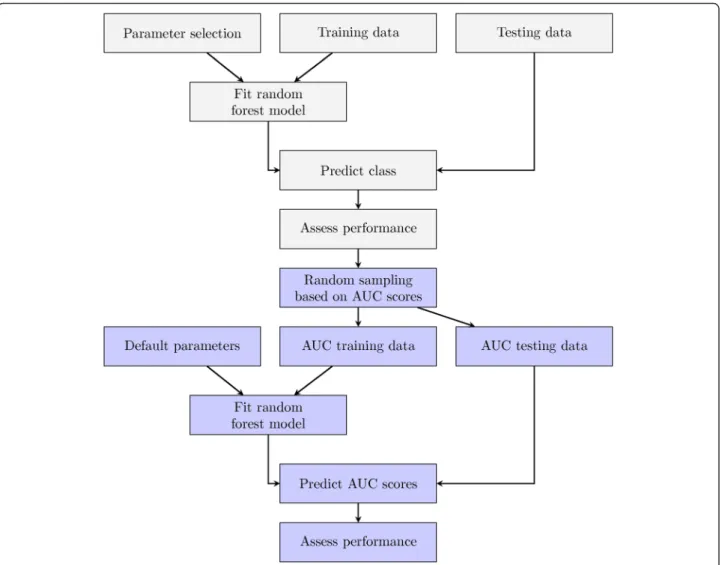
Fig. 1Experimental Design. Classification-based model fitting began with a unique combination ofntree,mtry, andsampsizeparameters in
conjunction with training data, illustrated by thegrayboxes. Each learned random forest model was used to predict the class of the validation data. Subsequently, AUC scores were calculated using the true class labels and these values were randomly subsetted into training and validation groups using 2/3 and 1/3 of the samples, respectively. In the second model fitting step, we evaluated whether AUC could be predicted from parameter sets alone. A RF regression model was fit using the parametersntree,mtry, andsampsizeas variables and AUC as the response, illustrated
by theblueboxes. Default settings were selected to train the RF regression models and AUC scores were predicted for the validation data. We evaluated the results using Spearman's and Lin’s correlation and determined the relative importance of each variable
While the results to this point demonstrate both that parameterization powerfully influences prediction accuracy and that the default parameter settings are sub-optimal. However they do not demonstrate if it is possible to improve upon the defaults via parameter-optimization studies. We therefore implemented 10-fold and stratified 10-fold cross-validation using the parame-ters in Additional file 1. The data was randomly divided into 10 even folds, using 9/10 folds for training and the last fold for validation. This step was repeated so that each fold was used for validation once, so that the number of samples in validation was equal to the number of samples in the original training set (n= 720). All validation folds were pooled to evaluate AUC and cross-validated models
were compared to non-cross-validated models using Spearman'sρand Lin'sρc(Additional file 2).
Predicted classes for both 10-fold cross-validation and stratified 10-fold cross-validation were weakly, but statistically-significantly correlated to the predicted classes for non-cross-validated results (Additional file 7a-b), and strongly correlated to one another (Additional file 7c).
We found that validation and stratified cross-validation resulted in 97 % of models having an AUC of 1, including the defaults. We used an additional metric, root mean squared error (RMSE) to break ties. The opti-mal model in 10-fold cross-validation (rank = 1, ntree=
500000, mtry= 10, sampsize= 720) had a RMSE of
0.00203, whereas the default model (rank = 579) had a
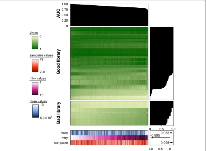
Fig. 2Prediction accuracy is a strong function of parameterization in lowp/nstudies. Summary of lowp/npredicted votes for each fitted random forest model (n= 1500). An AUC plot is provided at the top indicating the relative performance of each model, represented by each column. Each model was fitted from a unique combination ofntree(n= 10),mtry(n= 15) andsampsizeparameters (n= 10) and their respectively
outcomes (votes) for each sample or row (n= 576). Votes are provided in values from 0–1 with 0 representing a“bad library”and 1 representing a“good library”. All columns are ordered in descending order of AUC scores and rows are ordered in descending order of the fraction of correct votes for a given sample (total votes for the true sample class/all votes). All samples were subsetted according to the true class labels“good library”and“bad library”, though the votes may not be reflective of this. Barplots for vote fractions are provided on the right of the main heatmaps and the values for each parameter are provided at the bottom of the figure. Thentreeparameter is illustrated inblue,mtryinmagenta
andsampsizeinorange. Lighter hues represent lower values with darker hues indicating higher values. A scatterplot in the bottom right corner illustrates a strong negative correlation between themtryparameter with AUC scores (ρ= -0.89,p =0)
RMSE of 0.0273. The optimal model in stratified 10-fold cross-validation (rank = 1, ntree= 50, mtry= 14, sampsize
= 648) had a RMSE of 0.0119, whereas the default model (rank = 319) had a RMSE of 0.0229. Overall, we found that 39 % (578/1500) and 21 % (318/1500) of models outperformed the untuned model (ntree= 500, mtry= 3,
sampsize= 720), respectively. Twenty one percent (310/ 1500) of these models shared the same parameter values and were found to perform better than the default settings in both cross-validated and non-cross-validated results. We found the addition of a second metric, RMSE useful in breaking ties and assessing model performance for lowp/ndata.
Prediction accuracy can be a strong function of parameterization in highp/nstudies
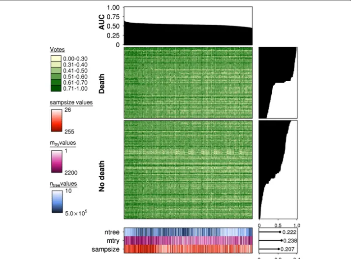
To contrast these data, we examined the effects of parameterization on prediction accuracy for high p/n data [13] (Additional file 1). We created 1,000 different sets of parameters and evaluated the performance of each (Additional file 8). Again, we saw that model per-formance varied greatly with parameterization with a median AUC of 0.533 and 2 % of models exceeding an AUC of 0.60 (Fig. 3). However, the performance varied dramatically, with a range of 0.4254–0.6337, suggesting that some parameterizations could greatly improve or hinder prediction accuracy. The default parameterization
Fig. 3Prediction accuracy is a strong function of parameterization in highp/nstudies. Summary of the predicted votes for the combined validation data for each fitted random forest model (n= 1000). A barplot for AUC scores is provided at the top indicating the relative performance of each model, represented by each column. Each model was fitted from a unique combination ofntree(n= 10),mtry(n= 10) andsampsizeparameters (n= 10)
and their respectively outcomes (votes) for each sample or row (n= 186). Votes are provided in values from 0–1 with 0 representing a“no death” event and 1 representing a“death”event. All columns are ordered in descending order of AUC scores and rows are ordered in descending order of the fraction of correct votes for a given sample (total votes for the true sample class/all votes). All samples were subsetted according to the true class labels“death”and“no death”, though the votes may not be reflective of this. On the right of the main heatmaps are respective barplots for vote fractions and a heatmap of parameter values is present at the bottom of the figure. Thentreeparameter is illustrated inblue,mtryinmagentaand sampsizeinorange. Lighter hues represent lower values with darker hues indicating higher values. To the right of this is a scatterplot illustrating Spearman's correlations of each parameter with the AUC scores; positive correlations were observed for the parametersntree,mtry, andsampsize
(ntree= 500, mtry= 110, sampsize= 255) performed well
relative to other models, with an AUC of 0.6098 and ranked 10th. This demonstrates the near optimal per-formance of the default settings.
We asked if models were consistently struggling with the same samples. We looked for samples in the valid-ation dataset where at least 50 % of models trained with different parameter sets made incorrect predictions. In total 89/186 (48 %) of validation samples were difficult to classify. These were symmetrically distributed be-tween the classes with 37/74 (50 %)“death” events diffi-cult to classify compared to 52/112 (46 %) “no death” samples (p= 0.74; proportion-test). The error rate was significantly different between these two groups (for “no death”samples;p= 0; proportion-test).
Parameterization was strongly correlated to AUC in this dataset, with contribution from all parameters. We observed that mtry (ρ= 0.238, p= 2.12 × 10⁻¹⁴;
Spear-man’s correlation) was the most correlated, followed by ntree(ρ= 0.222, p= 1.39 × 10⁻¹²; Spearman’s correlation)
and sampsize (ρ= 0.207, p= 3.73 × 10⁻¹¹; Spearman’s correlation).
To further explore the relationship between parameterization and performance, we univariately compared performance within each parameter (Additional file 1), with Benjamini-Hochberg adjustment for multiple-testing [39]. We observed that largerntree values resulted
in higher prediction accuracy and reduced performance variability compared to lower values (q< 10−8), with no significant difference observed between values ntree≥
10,000 (Additional files 9 and 10). Similar results were ob-served for sampsizeand mtry(Additional files 11 and 12)
where there was a near-linear relationship between in-creasing parameter values and AUC in the validation cohort. Additionally, no significant differences were ob-served in AUC forsampsize≥153 andmtry≥110. Themtry
value here is notable since it was used as the default, pro-viding some support to previous claims that the default performs well. These findings illustrated the strong influ-ence of parameter selection on classification accuracy, and that both linear and threshold effects can be observed.
Parameters can be used to predict performance
Having shown that model performance is strongly influ-enced by ntree, mtry, and sampsize, we next asked how
strongly these three parameters could predict AUC directly. We assessed variable importance using the Gini VIM, where larger values indicate a variable is more important for accurate classification. We were able to predict AUCs using this metric that closely reflects those of the true data for low p/n data (Additional file 13a;
ρ= 0.92, p= 1.29 × 10−209, ρc= 0.89; Spearman's ρ and
Lin's ρc). We observed that mtrydemonstrated the
high-est Gini VIM for lowp/ndata (Additional file 13b).
Similar results were observed for the high p/n data, where prediction accuracy was a strong function of par-ameter selection across all validation sets (Additional file 14a; ρ= 0.48, p= 5.42 × 10⁻²¹, ρc= 0.33; Spearman's ρ
and Lin'sρc). Interestingly, the parameters demonstrated
relatively balanced importance measures with sampsize demonstrating the highest Gini VIM and ntree with the
lowest (Additional file 14b).
Importance ranks can be sensitive to parameter changes
Finally, we asked if parameterization change could alter the identification of importance variables (which are fre-quently used in feature-selection approaches, for ex-ample) [23, 36]. We focused on the low p/n data, and trained models using the settings in Additional file 1 and ranked permutation VIM for each quality metric from 1–15, with 1 representing the most important variable. Permutation VIM is the mean decrease in classification accuracy after a random variable is removed from model fitting. Larger values suggest a variable has more dis-criminative power [40, 41].
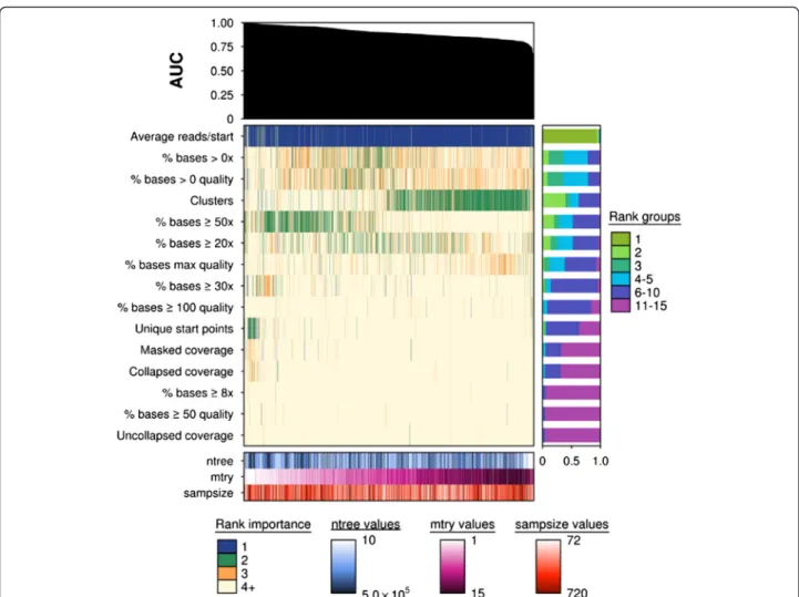
Variables differed in their sensitivity to parameter changes when evaluating variable importance (Fig. 4). The variable “Average reads/starts” was robust against parameter changes and was considered the most import-ant in 94 % of all samples, whereas “Clusters” exempli-fied strong parameter sensitivity and was positively correlated tomtry. On the other hand, “% bases≥50 %”
was found to have higher VIMs with lowermtryvalues.
Our order for variable importance deviated from that of the original study [6], where “% bases≥8×” was re-ported as the most discriminative variable. We examined how variable importance changed with differing ntree
values (n= 10) while holdingmtryandsampsize constant
(mtry= 3, sampsize= 720; Additional file 15) and
ob-served that largerntreevalues led to more stable VIMs.
Discussion
There are two common assumptions regarding RF models. The first is that the default parameters lead to good performance [37, 38] and the second is that the al-gorithm is robust to parameter changes [19, 21, 42]. To help quantify the wide-spread nature of these assump-tions we manually reviewed all papers published in BMC Bioinformatics between January 1, 2015 and November 21, 2015 (Additional file 16). We looked for papers that referenced the canonical RF paper [18] during this ~11 month period. Of the 16 papers that implemented RFs, exactly half performed a parameterization study to optimize parameters, and only 5/16 papers reported the final parameter setting used. That is, about half of RF-studies could benefit from improved parameterization and another third from improved reporting. This high-lights clearly the gap between machine learning theory
and practice, and gaps in methods reporting that are not being caught by peer-review.
Parameterization is difficult and its absence from the model fitting process may be due to limited experience, a lack of readily available heuristics or limited resources [43]. Consequently, these factors lead to the inappropri-ate selection of parameters or lack thereof, directly influencing learning [44]. We sought to determine the effects of parameterization on classification accuracy and variable importance measures. Our findings suggested
data-dependent parameter sensitivities ultimately influ-ence classification accuracy and VIMs for binary classifi-cation problems. Our findings may not extend to regression analyses or multi-class problems, where the relationship between the variables and response is much more complex.
We observed that the default parameters have the potential to perform well, however results across all tests indicated that parameter tuning enabled higher model performance. The majority of high performing parameter
Fig. 4Importance ranks can be sensitive to parameter changes in lowp/nstudies. Summary of the variable importance ranks for each sequencing metric (n= 15). An AUC plot is provided at the top indicating the relative performance of each model, represented by each column. Each model was fitted from a unique combination ofntree(n= 10),mtry(n= 15) andsampsizeparameters (n= 10) and their respectively outcomes (importance value)
for each metric. Each column of the main heatmap corresponds to a model's importance values, and were ranked from 1–15, where 1 represented the most important feature and 15 the least. The importance values were ordered according to previously calculated AUC scores using predicted vote and true class labels. Each row represents a metric and are ordered according to the mean rank of its importance values. The importance values were simplified in the main heatmap and illustrate four groups only.Blueindicates a rank of 1,greena rank of 2,golda rank of 3, andbeigea rank of 4 and greater. A summary of overall rank groups for a particular metric are illustrated in a barplot on the right of the main heatmap and a covariate heatmap with all parameter combinations is illustrated at the bottom of the plot. Thentreeparameter is illustrated inblue,mtryinpinkandorangeforsampsizein orange. Some parameters demonstrate robust behaviour to parameter changes such as“Uncollapsed coverage”and“% bases≥50 quality”, which were ranked between 11–15 inclusive in 96 % and 95 % of all samples, respectively. These variables possessed VIMs that suggested they were less influential on classification accuracy. Yet,“Average reads/starts”was insensitive to parameter changes and was considered the most important variable. Another variable“Clusters”was parameter sensitive, illustrating that variables vary in their sensitivity to parameter changes which can ultimately influence classification accuracy
combinations did not coincide with general patterns observed in the pattern selection process i.e., in most samples higher parameter values led to greater classifica-tion accuracy and the top performing parameters had lower values. Such models may have performed well due to random chance or were over-fit. These results emphasize the importance of parameter tuning and how one cannot rely on any arbitrary parameter set to perform well. This also suggests that existing publications imple-menting untuned models may improve classification ac-curacy through model tuning. To reduce computation time and work for parameter selection, we applied a RF regression model, which predicted model performance more accurately than the more expensive 10-fold cross-validation and stratified 10-fold cross-cross-validation. The RF regression model was also better at discriminating poor performing parameter sets from high performing param-eter sets.
To our knowledge, this is the first computational genomic study that addresses parameter sensitivities using a comprehensive range of values for two unique biological data types. In particular, we observed that the low p/n data was sensitive to changes in mtry and the
high p/n data demonstrated a synergism between all three parameters. Additionally, not all variables exhibited robust behaviour towards parameter changes when determining VIMs (e.g., “Clusters” and “% bases≥50×”). These findings challenge the assumption that RFs are relatively robust. Parameters that did not a play key role independently had an observable and significant syner-gism when constructing RF regression models with interaction terms (from section Parameters can be used to predict performance).
We also noted that our variable importance ranks did not coincide with [6]. This was largely explained by the bias in feature importance for the RF algorithm. Variables that were highly correlated to truly influential variables or have more categories will be over-selected by the algo-rithm and do not reflect the true relative contribution of a variable in a classification or regression problem [20]. Chong et al. [6] implemented an alternate algorithm,
“cforest”, from the R package“party”to generate unbiased VIMs. One area for future research is to investigate the sensitivity of parameter changes in the“cforest”algorithm. Moreover, characteristics of the data, such as, p > > n and minor class imbalances were observed. The numer-ous variables in the highp/ndata constrained the selec-tion range of mtry parameters, potentially confounding
the results. In such samples, mtry≠p. This was not the
sample for the lowp/n data, where we were able to test all possible values of mtry. This limitation may also be
viewed as beneficial since the number of randomly se-lected variables at each split is constrained and therefore, limits tree correlation within a forest.
An additional data characteristic limiting the classifica-tion accuracy in RF could be class imbalance [45, 46]. The unequal number of classes in a dataset is technically considered class imbalance, however, in the scientific community, class imbalance corresponds to data with significant to extreme disproportional class numbers, such as, 100:1 or 10,000:1 [47]. These types of “ imbal-anced data” were not considered here. Furthermore, the minor classes“bad library” and“death” in the small p/n data and highp/ndata respectively, had a higher classifi-cation accuracy suggesting, in some instances, the heterogeneity of a sample is more influential on classifi-cation accuracy. We also aimed to mitigate class imbal-ance effects through stratified sampling and by using the AUC performance metric. Alternate methods such as, cost sensitive learning [48] and artificially balancing the data through down sampling the majority class [49], over sampling the minority class [50], or both [51] have been shown to deal with class imbalance effectively. Artificial balancing ensures that class priors are equal in tree clas-sifiers and that the minority class is included in the bootstrap sample. On the other hand, cost sensitive learning incurs a greater cost for misclassified minority samples over majority samples. Minor class imbalances were not observed to be an issue in this study, however, data should be analysed with caution in highly imbal-anced studies.
Conclusions
We analysed the effects of parameterization using ex-haustive selection methods and showed that tuning can be successfully applied to a non-parametric machine learning algorithm to improve prediction accuracy. Although we only examined two different genomic sets, we observed that parameter sensitivities are data-specific, necessitating per-dataset tuning. Our findings illustrate this through discordant correlations between parameters and performance scores for lowp/nand high p/n data. The model fitting process is a fundamental step in machine learning and careless parameter selec-tion can lead to sub-optimal models and potentially missed findings.
Methods
Datasets
We explored parameterization of RFs on two datasets. The first was a sequencing-derived dataset (low p/n data) [6] and the second was a microarray-derived data-set (highp/ndata) [13], reflecting low and highp/ndata, respectively.
The lowp/ndata (15 variables with 1,296 samples) con-tained 15 quality metrics describing overall coverage, coverage distribution, basewise coverage and basewise quality of 53 whole genomes. The data was derived for the
International Cancer Genome Consortium (ICGC) project to predict the amount of sequencing that is required to reach a given coverage depth for 1/8 lane samples [6]. The outcome column was a list of binary values (0 for“bad li-brary” or 1 for“good library”) indicating whether the tar-get coverage depth was reached (30× for normal, 50× for tumour). The data was split into training and validation sets, as described by the lowp/npaper [6] and contained 720 and 576 samples, respectively.
The highp/n data contained gene expression data for 442 lung adenocarcinomas and basic clinical covariates (stage, age and sex) to predict lung cancer patient out-come (0 for “no death” or 1 for“death”). The data were collected from six contributing institutions and grouped into four subsets based on the laboratory where processed (University of Michigan Cancer Center (UM), Moffitt Cancer Center (HLM), Memorial Sloan-Kettering Cancer Center (MSKCC), and Dana-Farber Cancer Institute (DFCI)). All facilities processed the data using the same robust and reproducible protocol.
The first two datasets, UM and HLM, were grouped together to form the training set (12,138 variables with 255 samples), while the MSKCC data (104 samples) and DFCI data (82 samples) formed the validation set (186 samples).
Parameter selection
The mtry parameter values were selected using factor
levels of the default value. Since the nature of this super-vised learning problem is that of classification and not regression, the default value ofmtryis the square root of
the number of variables or features in the data 18 √p, whereas, in regression the default is p/3. The study by [21] reported mtry as the most sensitive parameter with
values of mtry factor = 1/2 (1/2• 18 √p), mtry factor = 1
(18 √p) and mtry factor = 2 (2•18√p) showing good
performance. Given this information and the number of variables in the data, one to all variables were selected as mtry values for the SeqControl dataset (p= 1-15), the
mtry values 1, 5, 11, 22, 55, 110, 220, 550, 1100, 2200
were selected for the NSCLC data (p= 12,138). The NSCLC values were obtained by selecting factor levels (1/100, 1/20, 1/10, 1/2, 1, 2, 5, 10, 20), multiplying them with pand taking the largest integer preceding a speci-fied number i.e., for a value of 3.4, 3 was used.
The values forntreewere selected similarly to those for
mtry. We imposed factor levels to the default value and
took the product to create the ntree values. The factor
levels were 1/50, 1/10, 1/5, 4/10, 1, 2, 20, 100, 200 and 1000. The final ntree values were 10, 50, 100, 200, 500,
1000, 1e4, 5e4, 1e5, 5e5. The selected ntree values were
the same for both datasets.
The final parameter sampsize, had the same factor levels for both datasets and was a sequence of values
from 0.1–1, increasing by increments of 0.1. To obtain the finalsampsizevalues, we multiplied the total number of samples in training by the sampsize factor levels and took the smallest integer proceeding a number i.e., for a value of 3.4, 4 was used.
Selected parameters were used to train models with the function “randomForest” using sampling with re-placement. The data was partitioned according to the original papers, as described above. In the SeqControl data experiment, we aimed to predict whether the target of sequencing depth coverage was achieved using 1/8 lane (1 for “good library”, 0 for “bad library”). In the NSCLC data experiment, we aimed to predict patient outcome (1 for “death”, 0 for “no death”). A table of complete parameter settings for the SeqControl data and NSCLC data can be found in Additional file 1.
Model training
The data were trained using the function “ randomFor-est” from the R package “randomForest” (v4.6-10) [21, 52]. A series of RFs were trained on each dataset using a unique combination of the three parameters: ntree, mtry
and sampsize. For the SeqControl data, we used 15mtry
values, 10 ntree values, and 10 sampsize values. These
values and numbers differed slightly in the NSCLC training: 10mtryvalues, 10ntree values, and 10sampsize
values. A resulting total of 1500 and 1000 unique com-bination were obtained for model fitting on the SeqCon-trol data and NSCLC data, respectively.
After training, each model was then validated on inde-pendent validation data to obtain class probabilities (votes). The votes and true class labels were then used to estimate model performance by calculating the AUC score.
Performance prediction using parameters as variables
In order to determine whether model performance could be predicted, we performed regression using RF, on a sub-set of parameters and their respective AUC scores. AUC scores were calculated by comparing the predicted votes from each model to the true classifications. We initially attempted this from a linear model approach, however, classification accuracy was low due to overfitting. After subsetting 2/3 of the data into training and 1/3 for valid-ation, we performed model tuning and selected the model with the lowest mean squared error. Tuning was con-ducted using a grid of parameters (Additional file 17) and 5-fold cross validation. We then applied the optimal set-tings (ntree= 200, mtry= 2, sampsize= 200) to train a RF
model. The response for our model was AUC score and the variables werentree,mtryandsampsize. The expression
for the model formula included the terms in an additive and interaction format i.e.,sampsize+mtry+ntree+
After training and validating the models, we were able to assess performance using the following metrics, Spear-man's ρ, Spearman's p-value (P) and Lin's ρc. Lastly,
importance values were found for each variable (ntree,mtry
orsampsize) in the form of Gini VIM.
Model selection using 10-fold cross-validation and stratified 10-fold cross-validation
Ten-fold cross-validation was used to estimate the generalization error of each unique RF model (n= 1500) for the SeqControl data. This method of cross-validation has been suggested to perform better than the more ex-pensive leave-one-out cross-validation [53]. The data was subsetted into 10 even folds, with nine groups se-lected for training and the last reserved for validation. This process was iterated until each fold was used in the validation stage once, so that the number of samples in validation was equal to the number of samples in the original training set (n= 720).
The above was repeated for stratified 10-fold cross-validation with an even distribution of the minority class among each fold. A total of 72 samples appeared in each fold with approximately 14 samples of the minority class and 58 of the majority class. AUC scores were used to estimate accuracy and correlations were calculated be-tween non-cross-validation, 10-fold cross-validation and stratified 10-fold cross-validation results. A table com-paring the above three methods is in Additional file 2.
Ranking variable importance
Additional information pertaining to variable importance was collected from training and validating the SeqCon-trol models using permutation VIM [54]. Permutation VIM can be interpreted as the mean decrease in accur-acy of a RF due to the removal of a variable. The magni-tude of the value is directly proportional to the relative contribution of a particular variable in classifying samples, that is, the greater the decrease or drop in ac-curacy, the more a feature is correlated to the response.
The model for the SeqControl data had additional set-tings that were implemented, such as “importance”,
“localImp”, “proximity” and “keep.inbag”. These argu-ments were all set to “TRUE” to keep results relatively consistent with the original paper [6].
Due to the exhaustive parameter selection method of grid searching, we parallelized jobs using Perl High Per-formance Computing Interface (HPCI) [55] and paralle-lized jobs further by using the R package, “foreach” (v1.4.2) [56].
Statistical model evaluation
We evaluated the performance of models using several statistical measures in the R statistical environment (v3.1.3) [57]. For classification accuracy, we calculated
the AUC using the predicted votes and the true class labels with the function “auc” from the package pROC (v1.8) [58]. For non-parametric tests comparing the parameter performance in classification, we used the function“cor”from the base“stats”package (v3.2.0) [57] to calculate Spearman's ρ and to find the correlation coefficient between the AUC scores and the parameter of interest. Spearman's ρ, Spearman's p-value and the equation for Lin's ρc from the paper [59] were used to
determine the correlation between true and predicted AUC values in performance prediction. All p-values were adjusted using the function “p.adjust” from the base “stats” package (v3.2.0), using the Benjamini-Hochberg procedure.
Data visualization
Figures were generated in the programming language LaTeX and in the R statistical environment (v3.1.3) using custom R scripts for the “lattice” (v0.2-31) [60] and
“latticeExtra”(v0.6-26) [61] packages. Additional files
Additional file 1:RF parameter settings. RF parameter settings for low
p/ndata (SeqControl;p= 15) and highp/ndata (NSCLC;p= 12,138). (CSV 515 bytes)
Additional file 2:AUC results for lowp/ndata. Lowp/nresults for prediction accuracy using AUC as the performance metric for non-validation results, 10-fold non-validation and stratified 10-fold cross-validation. Ranks indicate the relative performance of different models with lower ranks representing higher performing models i.e., a rank of 1 is the best model. The default settings (ntree= 500,mtry= 3,sampsize= 720)
are found on row 1502 of the table. (CSV 116 kb)
Additional file 3:Pairwiset-test results forsampsizeintra-parameter groups for the lowp/ndata. Allp-values were adjusted using a Benjamini-Hochberg procedure. There were no groups that differed significantly from each other. (TXT 333 bytes)
Additional file 4:Pairwiset-test results forntreeintra-parameter groups
for the lowp/ndata. Allp-values were adjusted using a Benjamini-Hochberg procedure. The onlyntreevalue found to differ from every other ntreegroup was 10. (TXT 456 bytes)
Additional file 5:Intra-parameter values display variation in lowp/n
studies. We evaluated the parameterssampsize,ntreeandmtryby
performing pairwise t-tests with a Benjamini-Hochberg adjustment. AUC scores were grouped by parameter values as indicated by a unique colour (orange forsampsize, blue forntreeand pink formtry), resulting in
10 groups forsampsize(n= 150), 10 groups forntree(n= 150) and 15
groups formtry(n= 100). A horizontal line is present in each plot,
indicating the median of the lowest parameter value. Parameter values forsampsizewere not found to differ significantly from each other, whereas,ntree= 10 differed significantly from every other group and all mtryvalues demonstrated a difference with at least one other group.
These findings suggest that lowerntreevalues were associated with lower
classification accuracy, with an opposite trend observed in themtry
parameter, where higher values were negatively correlated with classification accuracy. (TIFF 1373 kb)
Additional file 6:Pairwiset-test results formtryintra-parameter groups
for the lowp/ndata. Allp-values were adjusted using a Benjamini-Hochberg procedure. Eachsampsizegroup was found to differ from at least 12 other groups. (TXT 2 kb)
Additional file 7:Performance results are correlated between non-validation results, 10-fold non-validation and stratified 10-fold cross-validation. Correlations between non-cross-validation and cross-validation results of fitted random forest models to perform feature selection. (a) Non-cross-validation results were correlated to 10-fold Non-cross-validation results (ρ= 0.084,p< 0.01,ρc= 3.9 × 10⁻⁴). (b) Non-cross-validation results were
also correlated to stratified 10-fold cross-validation results (ρ= 0.1,p< 10−4,
ρc= 2.9 × 10⁻⁴). (c) A very strong correlation was observed between
strati-fied 10-fold cross-validation and 10-fold cross-validation (ρ= 0.65,p< 10−179,
ρc= 0.63) with minimum AUCs of 0.9967 and 0.9952, respectively and 97 %
of models overlapping at an AUC of 1. (TIFF 5780 kb)
Additional file 8:AUC results for highp/ndata. Validation results for all highp/nmodels (n= 1000) using the MSKCC data, DFCI data, and combined MSKCC and DFCI data. The AUC results and ranks are provided for each combination ofntree,mtryandsampsizeparameters. Lower ranks
represent higher model performance with 1 representing the most accurate model and 1000 representing the worst performing model. Logical columns are present to indicate whether a parameter set performed better than the default or well across all validation sets. Model performance was defined as good if the parameter set resulted in an AUC of > 0.6 across all validation sets. The default settings (ntree= 500, mtry= 110,sampsize= 255) are found on row 596 of the table. (CSV 28 kb)
Additional file 9:Intra-parameter values display variation for highp/n
studies (combined validation data). The parameterssampsize,ntreeand mtrywere analysed by performing pairwise t-tests with a
Benjamini-Hochberg adjustment. AUC scores were grouped by parameter values as indicated by colour (orange forsampsize, blue forntreeand pink formtry).
In general, lower intra-parameter values forsampsize,ntree, andmtrywere
found to differ significantly from higher intra-parameter values, with higher parameter values exhibiting a positive correlation with AUC. (TIFF 1207 kb)
Additional file 10:Pairwiset-test results forntreeintra-parameter groups
for the combined NSCLC validation data. Allp-values were adjusted using a Benjamini-Hochberg procedure. Lowerntreegroups were found to differ
from higherntreeparameter groups for example,ntree10 fromntree10,000 −500,000. (TXT 1019 bytes)
Additional file 11:Pairwiset-test results formtryintra-parameter groups
for the combined NSCLC validation data. Allp-values were adjusted using a Benjamini-Hochberg procedure. In general lowermtryvalues were
found to differ significantly from highermtryvalues for example,mtry1
frommtry110−2200. (TXT 1009 bytes)
Additional file 12:Pairwiset-test results forsampsizeintra-parameter groups for the combined NSCLC validation data. Allp-values were adjusted using a Benjamini-Hochberg procedure. Significant differences were observed between large and smallsampsizevalues, in particular,
sampsize26 fromsampsize102−255;sampsize51 fromsampsize128−255;
sampsize77 fromsampsize128−255, etc. (TXT 1 kb)
Additional file 13:AUC performance can be predicted for lowp/ndata using parameters as variables. Prediction accuracy (AUC) using the random forest classifier for lowp/ndata with Gini importance measures. (a) The model for the SeqControl data shows a strong correlation between predicted and observed AUC scores (ρ= 0.92,p< 10−208) and a Lin’s concordance correlation coefficient (ρc) value of 0.89. (b) The Gini
importance measures for the lowp/nAUC values show thatmtryis the
most informative variable followed byntreeandsampsize. (TIFF 80 kb)
Additional file 14:AUC performance can be predicted for highp/n
data using parameters as variables. Prediction accuracy using the random forest classifier for highp/nvalidation data with Gini importance measures. (a) The combined validation data demonstrated a strong correlation between the predicted and observed AUC values (ρ= 0.48,p< 10−20) and a
ρcvalue of 0.33. (b) The relative order of Gini importance for the combined
data wassampsizefollowed bymtryand lastly,ntree. (TIFF 68 kb)
Additional file 15:Variable importance ranks according tontreevalue. The ranks for the default parameters with uniquentreevalues as column
heads and sequencing quality metrics as row heads. The ranks stabilize at
ntree= 10,000. Using this criteria, the variable identified as the most
important was“Average reads/starts”in 40 % of samples, whereas, [6] identified“% bases≥8×”as the most important variable using the cforest
algorithm. Belowntree1,000,“% bases≥8×”was ranked as the most
important variable in 40 % of samples. Although greaterntreevalues may
lead to more consistent rankings for variable importance, these values may become more biased through sampling with replacement methods [20]. (CSV 667 bytes)
Additional file 16:Random forest usage in papers. A summary table of papers referencing random forest over a seven month period (January 1 to November 4) from BMC Bioinformatics. Information was recorded whether the paper uses a RF algorithm, and if so, whether they parameterized and report the tuned parameters. Eleven of sixteen papers use the RF algorithm and less than half of samples performed model tuning. An even fewer number of papers reported the optimized values [62–87]. (CSV 434 bytes)
Additional file 17:Parameter grid for predicting performance. A summary table of parameters that were used to perform model tuning for predicting AUC using a subset of parameters,ntree,mtryandsampsize.
A total of 162 parameters were used in model tuning and the optimal parameters (ntree= 200,mtry= 2,sampsize= 200) were selected to fit the
final model. (CSV 124 bytes)
Acknowledgements
We are grateful to the reviewers who have contributed to the significant improvement of this paper, and to all members of the Boutros laboratory for their technical support and insightful comments.
Funding
This study was conducted with the support of the Ontario Institute for Cancer Research to PCB through funding provided by the government of Ontario. Dr. Boutros was supported by a Terry Fox Research Institute New Investigator Award and a CIHR New Investigator Award. This work was supported by Prostate Cancer Canada and is proudly funded by the Movember Foundation - Grant #RS2014-01.
Availability of data and material
Using public datasets that are already available. Data from the SeqControl experiment may be accessed through the original paper from Nature Methods (http://www.nature.com/nmeth/journal/v11/n10/full/ nmeth.3094.html). The data used can be found in the Supplementary information as Supplementary table 10. Data from the lung adenocarcinoma study may be accessed through the original paper from Nature Medicine (http://www.nature.com/nm/journal/v14/n8/full/nm.1790.html). The microarray data can be found in the methods section of the paper and accessed at: https://www.ebi.ac.uk/arrayexpress/search.html?query=Affymetrix +lung+adenocarcinoma and accession number, E-GEOD-68571.
Authors’contributions
BFH: Performed statistical and bioinformatics analyses. BFH: Wrote the first draft of the manuscript. BFH, PCB: Initiated the project. PCB: Supervised research. All authors read and approved the final manuscript.
Competing interests
The authors declare that they have no competing interests.
Consent for publication
Not applicable.
Ethics approval and consent to participate
Not applicable.
Author details 1
Informatics and Bio-computing Program, Ontario Institute for Cancer Research, Toronto, Canada.2Department of Medical Biophysics, University of Toronto, Toronto, Canada.3Department of Pharmacology and Toxicology, University of Toronto, Toronto, Canada.4MaRS Centre, 661 University Avenue, Suite 510, Toronto, Ontario M5G 0A3, Canada.
References
1. Cruz JA, Wishart DS. Applications of Machine Learning in Cancer Prediction and Prognosis. Cancer Inform. 2006;2:59–77.
2. Chen X, Liu M. Prediction of protein–protein interactions using random decision forest framework. Bioinformatics. 2005;21:4394–400.
3. Nielsen H, Brunak S, von Heijne G. Machine learning approaches for the prediction of signal peptides and other protein sorting signals. Protein Eng Des Sel. 1999;12:3–9.
4. Burbidge R, Trotter M, Buxton B, Holden S. Drug design by machine learning: support vector machines for pharmaceutical data analysis. Comput Chem. 2001;26:5–14.
5. Murphy RF. An active role for machine learning in drug development. Nat Chem Biol. 2014;7:327–30.
6. Chong LC, Albuquerque MA, Harding NJ, Caloian C, Chan-seng-yue M, De Borja R, Fraser M, Denroche RE, Beck TA, Van Der KT, Bristow RG, Mcpherson JD, Boutros PC. SeqControl: process control for DNA sequencing. Nat Methods. 2014;11:1071–8.
7. Ben-Hur A, Ong CS, Sonnenburg S, Schölkopf B, Rätsch G. Support vector machines and kernels for computational biology. PLoS Comput Biol. 2008;4, e1000173.
8. Lafferty J, McCallum A, Pereira FCN. Conditional Random Fields : Probabilistic Models for Segmenting and Labeling Sequence Data. In: Proc 18th Int Conf Mach Learn. 2001. p. 282–9.
9. Statnikov A, Wang L, Aliferis CF. A comprehensive comparison of random forests and support vector machines for microarray-based cancer classification. BMC Bioinforma. 2008;9:1–10.
10. Guyon I, Weston J, Barnhill S. Gene Selection for Cancer Classification using Support Vector Machines. Mach Learn. 2002;46:389–422.
11. Hilario M, Kalousis A, Müller M, Pellegrini C. Machine learning approaches to lung cancer prediction from mass spectra. Proteomics. 2003;3:1716–9. 12. Tan AC, Gilbert D. Ensemble machine learning on gene expression data for
cancer classification. Appl Bioinforma. 2003;2:1–10.
13. Shedden K, Taylor JMG, Enkemann SA, Tsao MS, Yeatman TJ, Gerald WL, Eschrich S, Jurisica I, Giordano TJ, Misek DE, Chang AC, Zhu CQ, Strumpf D, Hanash S, Shepherd FA, Ding K, Seymour L, Naoki K, Pennell N, Weir B, Verhaak R, Ladd-Acosta C, Golub T, Gruidl M, Sharma A, Szoke J, Zakowski M, Rusch V, Kris M, Viale A, et al. Gene expression-based survival prediction in lung adenocarcinoma: a multi-site, blinded validation study. Nat Med. 2008;14:822–7.
14. Ayers M, Symmans WF, Stec J, Damokosh AI, Clark E, Hess K, Lecocke M, Metivier J, Booser D, Ibrahim N, Valero V, Royce M, Arun B, Whitman G, Ross J, Sneige N, Hortobagyi GN, Pusztai L. Gene expression profiles predict complete pathologic response to neoadjuvant paclitaxel and fluorouracil, doxorubicin, and cyclophosphamide chemotherapy in breast cancer. J Clin Oncol. 2004;22:2284–93.
15. Shipp M, Ross KN, Tamayo P, Weng AP, Kutok JL, Aguiar RCT, Gaasenbeek M, Angelo M, Reich M, Pinkus GS, Ray TS, Koval MA, Last KW, Norton A, Lister A, Mesirov J, Neuberg D, Lander ES, Aster JC, Golub TR. Diffuse large B-cell lymphoma outcome prediction by gene- expression profiling and supervised machine learning. Nat Med. 2002;8:68–74.
16. Liu JJ, Cutler G, Li W, Pan Z, Peng S, Hoey T, Chen L, Ling XB. Multiclass cancer classification and biomarker discovery using GA-based algorithms. Bioinformatics. 2005;21:2691–7.
17. Yasui Y, Pepe M, Thompson ML, Adam B-L, Wright JR GL, Qu Y, Potter JD, Winget M, Thornquist M, Feng Z. A data-analytic strategy for protein biomarker discovery: profiling of high-dimensional proteomic data for cancer detection. Biostatistics. 2003;4:449–63.
18. Breiman L. Random Forests. Mach Learn. 2001;45:5–32.
19. Díaz-Uriarte R, De Andrés SA. Gene selection and classification of microarray data using random forest. BMC Bioinforma. 2006;7:1–13.
20. Strobl C, Boulesteix A-L, Zeileis A, Hothorn T. Bias in random forest variable importance measures: illustrations, sources and a solution. BMC Bioinforma. 2007;8:25.
21. Liaw A, Wiener M. Classification and Regression by randomForest. R News. 2002;2:18–22.
22. Qi Y, Bar-Joseph Z, Klein-Seetharaman J. Evaluation of Different Biological Data and Computational Classification Methods for Use in Protein Interaction Prediction. Proteins. 2006;63:490–500.
23. Criminisi A, Shotton J, Konukoglu E. Decision Forests: A Unified Framework for Classification, Regression, Density Estimation, Manifold Learning and Semi-Supervised Learning. Found Trends® Comput Graph Vis. 2011;7:81–227.
24. Efron B, Tibshirani R. Introduction to the Bootstrap. New York: Chapman & Hall; 1993.
25. Svetnik V, Liaw A, Tong C, Culberson JC, Sheridan RP, Feuston BP. Random forest: a classification and regression tool for compound classification and QSAR modeling. J Chem Inf Comput Sci. 2003;43:1947–58.
26. Breiman L. Out-of-Bag Estimation. 1996. p. 1–13. 27. Breiman L. Bagging Predictors. Mach Learn. 1996;24:123–40.
28. Breiman L. Heuristics of Instability and Stabilization in Model Selection. Ann Stat. 1996;24:2350–83.
29. Hastie T, Tibshirani R, Friedman J. The Elements of Statistical Learning: Data Mining, Inference, and Prediction. 2nd ed. New York: Springer; 2005. 30. Segal MR. Machine Learning Benchmarks and Random Forest Regression.
2004.
31. Bauer E, Kohavi R. An Empirical Comparison of Voting Classification Algorithms : Bagging, Boosting, and Variants. Mach Learn. 2011;38:1–38. 32. Dietterich TG. An Experimental Comparison of Three Methods for
Constructing Ensembles of Decision Trees: Bagging, Boosting, and Randomization. Mach Learn. 2000;40:139–57.
33. Opitz D, Maclin R. Popular Ensemble Methods: An Emperical Study. J Artif Intell Res. 1999;11:169–98.
34. Nagi S, Bhattacharyya DK. Classification of microarray cancer data using ensemble approach. Netw Model Anal Heal Informatics Bioinforma. 2013;2: 159–73.
35. Snoek J, Larochelle H, Adams RP. Practical Bayesian Optimization of Machine Learning Algorithms. Adv Neural Inf Process Syst. 2012;1–9. 36. Okun O, Priisalu H. Random Forest for Gene Expression Based Cancer
Classification: Overlooked Issues. In: Proc 4th Int Meet Comput Intell Methods Bioinforma Biostat Portofino, Italy. 2007. p. 483–90.
37. Sun YV, Bielak LF, Peyser PA, Turner ST, Sheedy PF, Boerwinkle E, Kardia SLR. Application of machine learning algorithms to predict coronary artery calcification with a sibship-based design. Genet Epidemiol. 2008;32:350–60. 38. Sun YV. Multigenic Modeling of Complex Disease by Random Forest. Adv
Genet. 2010;72:73–99.
39. Benjamini Y, Hochberg Y. Benjamini and Y FDR.pdf. J R Stat Soc Ser B. 1995; 57:289–300.
40. Archer KJ, Kimes RV. Empirical characterization of random forest variable importance measures. Comput Stat Data Anal. 2008;52:2249–60. 41. Calle ML, Urrea V. Letter to the editor: Stability of Random Forest
importance measures. Brief Bioinform. 2011;12:86–9.
42. Goldstein BA, Briggs FBS, Polley EC. Random Forests for Genetic Association Studies. Stat Appl Genet Mol Biol. 2011;10:1–34.
43. Domingos P. A few useful things to know about machine learning. Commun ACM. 2012;55:78–87.
44. Li J-B, Chu S-C, Pan J-S. Kernel Learning Algorithms for Face Recognition. New York: Springer; 2013. p. 1–17.
45. Dudoit S, Fridlyand J. Classification in microarray experiments. Stat Anal gene Expr microarray data. 2003;1:93–158.
46. Sun Y, Kamel MS, Wong AKC, Wang Y. Cost-sensitive boosting for classification of imbalanced data. Pattern Recognit. 2007;40:3358–78. 47. He H, Garcia EA. Learning from Imbalanced Data. IEEE Trans Knowl Data Eng.
2009;21:1263–84.
48. Domingos P. MetaCost: A General Method for Making Classifiers. In: Proceedings of the 5th ACM SIGKDD International Conference on Knowledge Discovery and Data Mining. San Diego: ACM Press; 1999. p. 155–64.
49. Kubat M, Matwin S. Addressing the Curse of Imbalanced Training Sets: One-Sided Selection. In: Kaufmann M, editor. Proceedings of the 14th International conference on Machine Learning. 1997. p. 179–86. 50. Ling CX, Li C. Data Mining for Direct Marketing : Problems and Solutions.
In: Proceedings of the Fourth International Conference on Knowledge Discovery and Data Mining. New York: AAAI Press; 1998.
51. Chawla NV, Bowyer KW, Hall LO. SMOTE: Synthetic Minority Over-sampling Technique. J Artif Intell Res. 2002;16:321–57.
52. Breiman L, Cutler A, Liaw A, Wiener M. Breiman and Cutler’s random forests for classification and regression. 2015.
53. Kohavi R. A Study of Cross-Validation and Bootstrap for Accuracy Estimation and Model Selection. In: Kaufmann M, editor. International Joint Conference on Artificial Intelligence (IJCAI). 1995. p. 1137–43.
54. Leo Breiman. Manual - Setting up, using, and udnerstanding random forests v4.0. https://www.stat.berkeley.edu/~breiman/Using_random_ forests_v4.0.pdf.
55. Boutros lab. HPCI. http://search.cpan.org/dist/HPCI/.
56. Revolution Analytics. doMC: Foreach parallel adaptor for the multicore package. 2014.
57. R Core Team. R: A language and environment for statistical computing. 2015. 58. Robin X, Turck N, Hainard A, Tiberti N, Lisacek F, Sanchez J-C, Müller M.
pROC: an open-source package for R and S+ to analyze and compare ROC curves. BMC Bioinforma. 2011;18:77.
59. Lin LI. A Concordance Correlation Coefficient to Evaluate Reproducibility. Biometrics. 1989;45:255–68.
60. Sarkar D. Lattice: Multivariate Data Visualization with R. New York: Springer; 2008. 61. Sarkar D, Andrews F. latticeExtra: Extra Graphical Utilities Based on Lattice. 2013. 62. Sun J, Zhao H. The application of sparse estimation of covariance matrix to
quadratic discriminant analysis. BMC Bioinforma. 2015;16:48.
63. Shankar J, Szpakowski S, Solis NV, Mounaud S, Liu H, Losada L, Nierman WC, Filler SG. A systematic evaluation of high-dimensional, ensemble-based regression for exploring large model spaces in microbiome analyses. BMC Bioinforma. 2015;16:31.
64. Wu AC-Y, Rifkin SA. Aro: a machine learning approach to identifying single molecules and estimating classification error in fluorescence microscopy images. BMC Bioinforma. 2015;16:102.
65. Lee J, Lee K, Joung I, Joo K, Brooks BR, Lee J. Sigma-RF: prediction of the variability of spatial restraints in template-based modeling by random forest. BMC Bioinforma. 2015;16:94.
66. Limongelli I, Marini S, Bellazzi R. PaPI: pseudo amino acid composition to score human protein-coding variants. BMC Bioinforma. 2015;16:123. 67. Hofner B, Boccuto L, Göker M. Controlling false discoveries in
high-dimensional situations: boosting with stability selection. BMC Bioinforma. 2015;16:144.
68. Fratello M, Serra A, Fortino V, Raiconi G, Tagliaferri R, Greco D. A multi-view genomic data simulator. BMC Bioinforma. 2015;16:151.
69. Ruiz-Blanco YB, Paz W, Green J, Marrero-Ponce Y. ProtDCal: A program to compute general-purpose-numerical descriptors for sequences and 3D-structures of proteins. BMC Bioinforma. 2015;16:162.
70. Sanders J, Singh A, Sterne G, Ye B, Zhou J. Learning-guided automatic three dimensional synapse quantification for drosophila neurons. BMC Bioinforma. 2015;16:177.
71. Schönenberger F, Deutzmann A, Ferrando-May E, Merhof D. Discrimination of cell cycle phases in PCNA-immunolabeled cells. BMC Bioinforma. 2015;16:180. 72. Novianti PW, Jong VL, Roes KCB, Eijkemans MJC. Factors affecting the
accuracy of a class prediction model in gene expression data. BMC Bioinforma. 2015;16:199.
73. Cheng X, Cai H, Zhang Y, Xu B, Su W. Optimal combination of feature selection and classification via local hyperplane based learning strategy. BMC Bioinforma. 2015;16:219.
74. Ogoe HA, Visweswaran S, Lu X, Gopalakrishnan V. Knowledge transfer via classification rules using functional mapping for integrative modeling of gene expression data. BMC Bioinforma. 2015;16:226.
75. Kuhring M, Dabrowski PW, Piro VC, Nitsche A, Renard BY. SuRankCo: supervised ranking of contigs in de novo assemblies. BMC Bioinforma. 2015;16:240. 76. Khurana JK, Reeder JE, Shrimpton AE, Thakar J. GESPA: classifying nsSNPs to
predict disease association. BMC Bioinforma. 2015;16:228.
77. Ren H, Shen Y. RNA-binding residues prediction using structural features. BMC Bioinforma. 2015;16:249.
78. Serra A, Fratello M, Fortino V, Raiconi G, Tagliaferri R, Greco D. MVDA: a multi-view genomic data integration methodology. BMC Bioinforma. 2015;16:261.
79. Korir PK, Geeleher P, Seoighe C. Seq-ing improved gene expression estimates from microarrays using machine learning. BMC Bioinforma. 2015;16:286.
80. Sakellariou A, Spyrou G. mAPKL: R/ Bioconductor package for detecting gene exemplars and revealing their characteristics. BMC Bioinforma. 2015;16:291. 81. Huang H, Fava A, Guhr T, Cimbro R, Rosen A, Boin F, Ellis H. A methodology
for exploring biomarker-phenotype associations: application to flow cytometry data and systemic sclerosis clinical manifestations. BMC Bioinforma. 2015;16:293.
82. Blagus R, Lusa L. Boosting for high-dimensional two-class prediction. BMC Bioinforma. 2015;16:300.
83. Bellot P, Olsen C, Salembier P, Oliveras-Vergés A, Meyer PE. NetBenchmark: a bioconductor package for reproducible benchmarks of gene regulatory network inference. BMC Bioinforma. 2015;16:312.
84. König C, Cárdenas MI, Giraldo J, Alquézar R, Vellido A. Label noise in subtype discrimination of class C G protein-coupled receptors: A systematic approach to the analysis of classification errors. BMC Bioinforma. 2015;16:314. 85. Cremona MA, Sangalli LM, Vantini S, Dellino GI, Pelicci PG, Secchi P, Riva L.
Peak shape clustering reveals biological insights. BMC Bioinforma. 2015;16:349. 86. Ditzler G, Morrison JC, Lan Y, Rosen GL. Fizzy: feature subset selection for
metagenomics. BMC Bioinforma. 2015;16:358.
87. Landoni E, Miceli R, Callari M, Tiberio P, Appierto V, Angeloni V, Mariani L, Daidone MG. Proposal of supervised data analysis strategy of plasma miRNAs from hybridisation array data with an application to assess hemolysis-related deregulation. BMC Bioinforma. 2015;16:388.
• We accept pre-submission inquiries
• Our selector tool helps you to find the most relevant journal
• We provide round the clock customer support
• Convenient online submission
• Thorough peer review
• Inclusion in PubMed and all major indexing services
• Maximum visibility for your research Submit your manuscript at
www.biomedcentral.com/submit