Full text document (pdf)
Copyright & reuse
Content in the Kent Academic Repository is made available for research purposes. Unless otherwise stated all content is protected by copyright and in the absence of an open licence (eg Creative Commons), permissions for further reuse of content should be sought from the publisher, author or other copyright holder.
Versions of research
The version in the Kent Academic Repository may differ from the final published version.
Users are advised to check http://kar.kent.ac.uk for the status of the paper. Users should always cite the published version of record.
Enquiries
For any further enquiries regarding the licence status of this document, please contact:
If you believe this document infringes copyright then please contact the KAR admin team with the take-down information provided at http://kar.kent.ac.uk/contact.html
Citation for published version
Oduro, Samuel Dua (2016) Bayesian econometric modelling of informed trading, bid-ask spread
and volatility. Doctor of Philosophy (PhD) thesis, University of Kent,.
DOI
Link to record in KAR
http://kar.kent.ac.uk/61094/
Document Version
informed trading, bid-ask spread
and volatility
Samuel Dua Oduro
Centre for Actuarial Science, Risk and Investment
School of Mathematics, Statistics and Actuarial Science
University of Kent
This dissertation is submitted in the subject of Actuarial Science for
the degree of
Doctor of Philosophy
And to my wife Joyce and children Loretta, Rodney, Phoebe and Nathaniel whose sacrifices has seen me through this journey.
I hereby declare that except where specific reference is made to the work of others, the contents of this dissertation is original and has not been submitted in whole or in part for consideration for any other degree or qualification in this, or any other University. This dissertation is the result of my own work and includes nothing which is the outcome of work done in collaboration, except where specifically indicated in the text.
Samuel Dua Oduro September 2016
To God, I give thanks for his protection through this academic journey. May His name be praised. The thesis has been made possible through the contributions of numerous individuals whom I was privilege to meeting at Kent. Firstly I would like to express my profound gratitude to Professor Jim E. Griffin and Dr Jaideep S. Oberoi who constituted my joint-supervisory team. I am indeed very thankful for their immense guidance, support, constructive criticism and detailed scrutiny of the entire research work. It was a rare privilege to work with such intelligent, friendly, firm and ac-commodating gentlemen. Secondly, I would like to thank the School of Mathematics, Statistics and Actuarial Science for the generous funding which enabled me focus on my research. I would like to thank Professor David Veredas of Vlerick Business School in Belgium for agreeing to examine this thesis. I am most grateful to him. To Mrs Claire Carter, our wonderful and always cheerful postgraduate research officer, I say
Tapadh leibh. You have always been there to support me not only on administrative procedures but personal life issues as well. Special thanks to Dr Dhirendra Kumar Sakaria, Dr Evangelia Mitrodima and Dr Abera Ayalew Muhamed for their friend-ship and support when the going went though in Canterbury. I appreciate the time I shared with you all. I am also very indebted to my mother-inlaw Madam Felicia Afia Asantewaa who took care of my children while I was away in Canterbury. I would like to appreciate Mr Samuel Mireku Agyapong and his wife Faustina Acheampong for the invaluable support to myself and my family before and during my relocation to Canterbury. Sincere thanks to my brother Mr Emmanuel Kwame Oduro and sis-ter Mrs Giftina Appiah-Agyei Sarpong for their prayer support. Finally, I am very indebted to my wife Joyce and children Loretta, Rodney, Phoebe and Nathaniel who endured my absence while I was in Canterbury far away from home. No amount of financial reward will suffice the patience you had for me on occasions when I indirectly extended my frustration from this research to you. God bless you all.
Recent developments in global financial markets have increased the need for research aimed at the measurement and possible reduction of liquidity risk. In particular, market crashes have been partly blamed on the sudden withdrawal of liquidity in markets and increases in liquidity risk. To this end, it is important to develop bet-ter approaches for inferring or quantifying liquidity risk. Liquidity risk caused by some investors trading on their information advantage (informed trading) has been a subject of market microstructure research in the last few decades. Researchers have employed information-based models that use observed or inferred order flow to inves-tigate this problem. The Probability of Informed Trading (PIN) is a measure which uses inferred order flow to quantify the extent information asymmetry. However, a number of computational issues have been reported to effect the estimation of PIN. Using an alternative methodology, we address the numerical problem associated with the estimation of PIN. Varied evidence of a relationship between volume and bid-ask spread has been documented in the extant literature. In particular, theory suggests that bid-ask spread and volume are jointly driven by a common process as both vari-ables measure an aspect of liquidity. The complex relationship between these varivari-ables is time-varying since the informed trading component of order flow changes as trading takes place. Thus, volume and bid-ask spread may provide insight on the time-varying composition of economic agents trading an asset. We exploit the nonlinear relation-ship between traded volume and bid-ask spread to develop a model that can be used to infer informed and uninformed trading components of volume. The structure of the model and estimation methodology enhances the sequential processing and incor-poration of past volume and bid-ask spread as conditioning information. The model is applied to two equities that trade on the New York Stock Exchange. Finally, to increase our understanding on the effects of liquidity risk on volatility, we also exam-ine whether separating volume into informed and uninformed components can provide further insight on the relationship between liquidity risk and volatility.
Contents xi
List of Figures xiii
List of Tables xv
1 Introduction 3
1.1 Measuring Information Asymmetry . . . 5
1.1.1 Spread decomposition models . . . 5
1.1.2 Price Impact Models . . . 6
1.1.3 Vector Autoregressive (VAR) Models . . . 7
1.1.4 Probability of Informed Trading (PIN) . . . 8
2 A Bayesian Approach To Probability Of Informed Trading 13 2.1 Introduction . . . 13
2.2 The Benchmark PIN Model . . . 15
2.3 Bayesian Inference Of Benchmark Model . . . 20
2.3.1 Method 1 : Gibbs Sampler . . . 21
2.3.2 Method 2: Metropolis-Hastings Algorithm . . . 27
2.4 Extension Of The Benchmark PIN Model . . . 30
2.5 Bayesian Inference Of The Extended PIN Model . . . 35
2.5.1 Method 1: Gibbs Sampler . . . 35
2.5.2 Method 2: Metropolis-Hastings Algorithm . . . 40
2.6 Hypothetical Data Implementation . . . 42
2.7 Real Data Estimation . . . 49
2.7.1 Discussion . . . 59
3 Estimating Daily Information Asymmetry Risk From High Frequency
Data 63
3.1 Introduction . . . 64
3.2 Empirical Analysis . . . 68
3.3 Concluding Remarks . . . 73
4 Learning About Informed Trading Via Volume - Spread Relationship 75 4.1 Introduction . . . 75
4.2 The Model . . . 82
4.3 Empirical Analysis . . . 93
4.4 Concluding Remarks . . . 102
5 Investigating The Link Between Volatility, Informed And Uninformed Trading 105 5.1 Introduction . . . 105
5.2 The Models . . . 108
5.3 Model Estimation . . . 113
5.4 Empirical Analysis . . . 118
5.5 One Day Ahead Volatility Forecasting . . . 126
5.6 Concluding Remarks . . . 134
6 Conclusions And Further Research 137
2.1 Information and order arrival process in Easley et al. (1996) model . . . 16
2.2 Information and order arrival process in Easley et al. (2002) model . . . 30
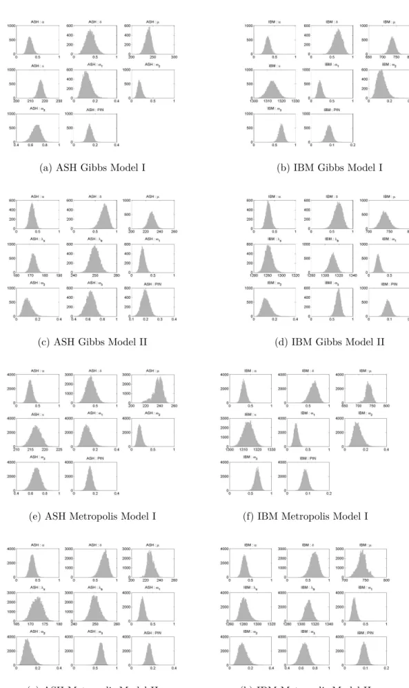
2.3 Posterior distributions for the simulated data of size 60 . . . 47
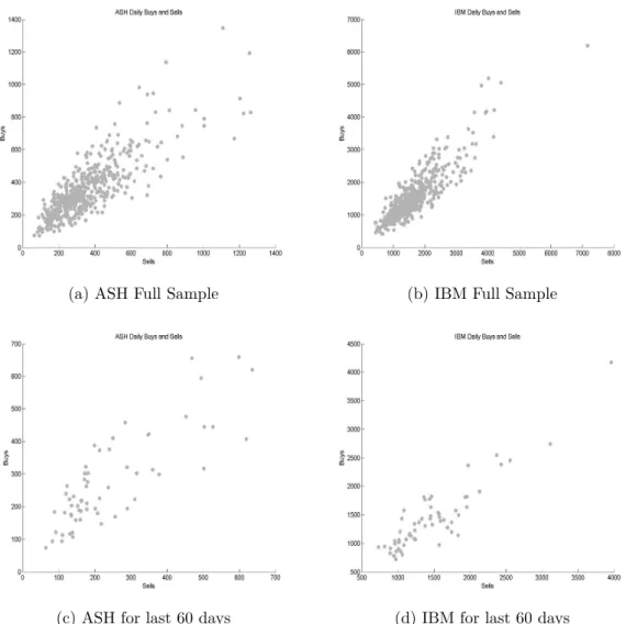
2.4 Daily buy and sell orders . . . 50
2.5 Posterior estimates for recent 60 trading days . . . 57
2.6 Posterior estimates for entire sample . . . 58
3.1 Comparison of daily PIN and VPIN . . . 72
4.1 Model A1 - Posterior distributions of parameters . . . 96
4.2 ASH model A1 - latent processes, volume and relative spread . . . 98
4.3 IBM model A1 - latent processes, volume and relative spread . . . 99
4.4 Model A2 - latent processes . . . 100
4.5 Comparison of daily PIN andht . . . 101
5.1 ASH - realized variance compared with ht and τt . . . 124
5.2 IBM - realized variance compared with ht and τt . . . 125
5.3 Benchmark models - comparison of one day ahead volatility forecasts. . 127
5.4 HAR versus other models - comparison of one day ahead volatility fore-casts. . . 128
5.5 ASH - Comparison of one day ahead volatility forecasts . . . 129
2.1 Parameter values for simulated data . . . 42
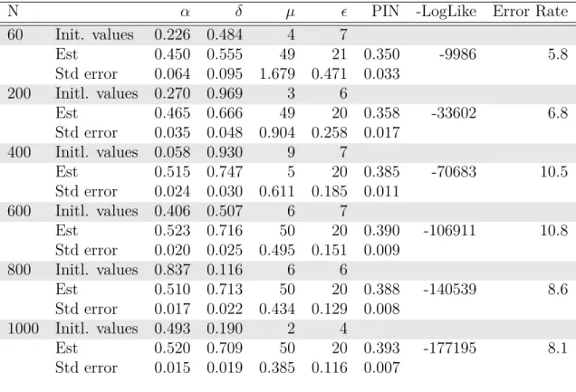
2.2 Maximum likelihood estimates of the simulated data for Model I . . . . 43
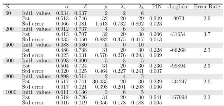
2.3 Maximum likelihood estimates of the simulated data for Model II . . . 44
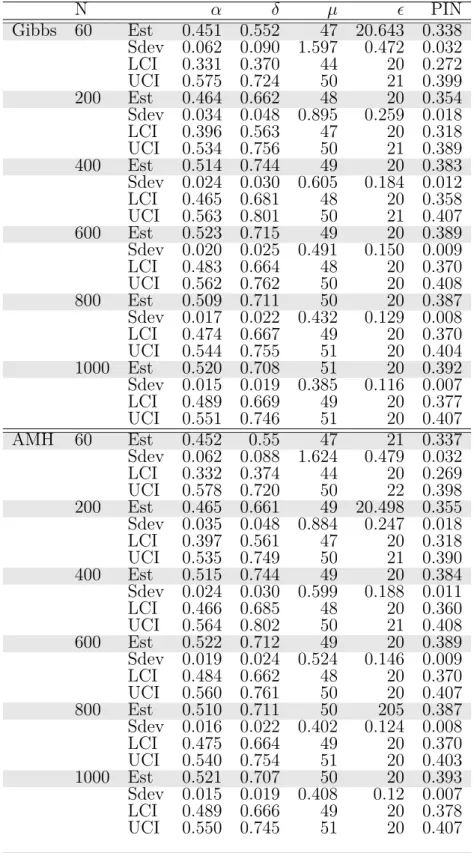
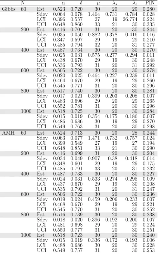
2.4 Posterior estimates of the simulated data for Model I . . . 45
2.5 Posterior estimates of the simulated data for Model II . . . 46
2.6 MLE for simulated data based on Noah Stoffman SAS1code . . . 48
2.7 Summary of daily buy and sell trades . . . 49
2.8 Maximum likelihood estimates of real data for Model I . . . 51
2.9 Maximum likelihood estimates of the real data for Model II . . . 51
2.10 MLE from Stoffman SAS code on real data . . . 52
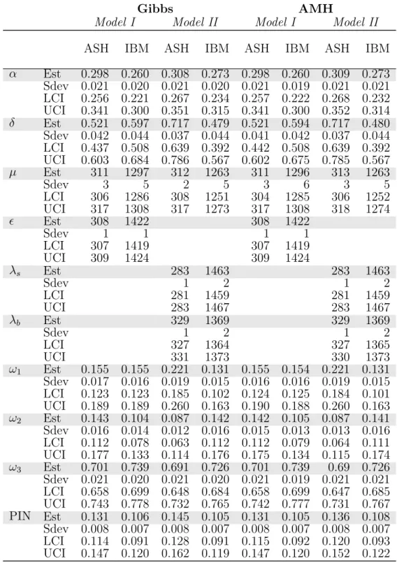
2.11 Posterior Estimates for the full sample . . . 53
2.12 Posterior estimates for last 60 days . . . 56
3.1 Summary of high frequency buy and sell trades . . . 68
3.2 Summary of daily PIN estimates . . . 69
3.3 Summary of VPIN . . . 70
4.1 Descriptive statistics of data . . . 93
4.2 Model A1 - Posterior estimates . . . 94
4.3 Model A2 - Posterior estimates . . . 94
5.1 Estimates from benchmark models . . . 118
5.2 ASH - Posterior estimates . . . 119
5.3 IBM - Posterior estimates . . . 120
5.4 RMSE and LPS of one day ahead volatility forecasts . . . 132
Introduction
Financial markets provide platforms for diverse participants including private in-vestors, institutional inin-vestors, brokers and designated market-makers to trade finan-cial securities. In addition to the facilitation of trade between market participants, the markets collect and make available trade-related information such as prices, traded volume, time of trade, number of transactions and other relevant variables about as-sets. Market participants take account of this information when they make purchase and sale decisions.
Academic researchers also use the trade-related information from financial markets to develop theories and models that can be used to learn about the trading behaviour of market participants. A branch of the finance literature that studies investor trading behaviour in financial markets is called market microstructure. This research area has been defined differently by several academics. A common definition that can be drawn from papers including Madhavan (2000), O’Hara (1995) and Spulber (1996) is that market microstructure explores the evolution of asset prices while taking into consideration the following micro-level market issues:
1. The effect of market regulations and mechanisms on the evolution of asset prices. 2. How well the organisation of markets enhances the easy exchange of assets in
large volumes with little or no impact on the price of the asset (liquidity). 3. How information generated from the demand and supply decisions of market
Market microstructure theory assumes that financial market participants have differ-ent information sets which influence their trading behaviour. Market participants, therefore, reveal the information they hold about the asset through their demand and supply decisions. Depending on the quality of information available, market partici-pants alter their expectations on the stream of future cash-flow of an asset and hence the value they place on the asset.
At the core of the extant literature, economic agents in financial markets are cate-gorised into informed and uninformed. The uninformed market participants are some-times referred to as liquidity traders. This categorisation is based on the assumed motives behind the trading decisions of market participants. Informed market partic-ipants are considered to have superior knowledge or the sophistication to determine whether an asset is mis-priced. They, therefore, enter into trades hoping to gains from their information advantage. On the other hand, uninformed market participants do not have any information on the future price of the asset and hence trade on a multi-tude of reasons. These reasons may include portfolio re-balancing, the need for funds for other investment projects and consumption smoothing.
The likelihood of a market participant entering into a transaction with other market participants who may potentially have superior knowledge about the value of the asset creates what is referred to as information asymmetry. Bagehot (1971) made the ar-gument that the differences between the prices at which investors are able and willing to buy or sell (bid-ask spread) an asset exist because some investors possess superior information. This implies that the size of the bid-ask spread is a function of informa-tion asymmetry. Informainforma-tion asymmetry is a fundamental source of uncertainty faced by market makers and liquidity providers. Investigating the presence or otherwise of informed trading in an asset and within the market is very important since information asymmetry affects the liquidity of an asset and the market in general.
In a seminal paper, Glosten and Milgrom (1985) formally presented a theoretical model for the idea of Bagehot (1971). According to Glosten and Milgrom (1985) traders arrive at the market sequentially to have their orders executed. In their model bid and ask prices are set based on the liquidity providers’ belief of the proportion of informed traders in the market. Thus in the absence of exogenous transaction cost there exist a positive bid-ask spread. On the other hand, Kyle (1985) postulates
that informed traders submit their orders strategically in a gradual manner. This strategic behaviour of informed traders ensures that the impact of their trades on asset price is minimal. Some academic papers have subsequently explored the information asymmetry problem by extending the work of Glosten and Milgrom (1985). Many papers based on initial work of Kyle (1985) also explore the impact of information asymmetry on trading cost.
Papers including Chordia et al. (2001), Acharya and Pedersen (2005), Brennan and Subrahmanyam (1996) and Easley and O’Hara (2003) argue that in equilibrium, high levels of information asymmetry create significant trading costs. This causes unin-formed traders to demand higher returns resulting in assets being purchased at a discount. Chordia et al. (2001) also indicate that information asymmetry affects the volatility of assets. French and Roll (1986) found evidence of increased price volatil-ity principally caused by private information of informed traders. Using a theoretical model, Wang (1993) also argues that in a market with information asymmetry, less informed traders demand an extra premium for the uncertainty of trading against bet-ter informed traders. Price volatility will, therefore, increase as less informed traders post quotes that widen the bid-ask spread.
1.1
Measuring Information Asymmetry
A number of approaches have been taken in the market microstructure literature to provide proxies for and measures of information asymmetry. In what follows we provide a brief review of some of the prominently used methods. This review however is not intended to be an exhaustive review of the numerous methods in the literature.
1.1.1
Spread decomposition models
A basic measure of illiquidity is the bid-ask spread. The bid-ask spread measures the rent market-makers charge for the provision of immediate liquidity. The adverse selection theory put forward by Glosten and Milgrom (1985) suggests that a trader offering to sell a large amount of his/her stock holdings unexpectedly will have to take a lower price for the asset if the counter-party to the trade believes that the seller of the stock has information which other traders do not know.
Various authors including Glosten and Harris (1988), foster1993variations, Madhavan et al. (1997), Huang and Stoll (1997) and Sadka (2006), have used a trade indicator regression model to decompose the bid-ask spread intoinventory-holding cost, adverse-selection cost and order-processing cost components. Liquidity suppliers incorporate into the bid-ask spread the costs associated with the execution and processing of orders they receive. These may include costs such as brokerage fees and transaction tax. Apart from these costs, liquidity providers are exposed to the risk of trading with better informed traders. The adverse-selection component of the bid-ask spread is the compensation demanded by liquidity traders for trading with informed traders. Also, since market makers hold inventory to meet their obligation of providing immediate liquidity when demanded, they are exposed to price changes. Hence they demand compensation for this price risk in the form of inventory-holding cost.
Let changes in mid-quote that prevailed before the transaction at time t be denoted as rt = (p
ask
t +pbidt )/2−(paskt−1+pbidt−1)/2. Buyer and seller initiated trades at time t are also
denoted by qt = +1 and qt = −1 respectively. If St is the quoted spread prior to
the transaction at time t, then the Huang and Stoll (1997) model which encompasses many of the trade indicator models is of the form
rt= (α+β) St−1 2 qt−1+α(1−2π) St−2 2 qt−2+εt, εt∼ N(0, σ 2), (1.1)
where E[qt−1♣qt−2] = (1−2π)qt−2. The model parameters α and β are the adverse
selection and inventory components of the quoted spread. The order processing com-ponent is calculated as 1−α−β. The probability that the trade at timetis opposite in sign to the trade att−1 is π. The adverse selection component is used as a proxy for information asymmetry. A temporary increase in the information asymmetry between the informed and uninformed investors should cause a temporary positive deviation in the bid-ask spread from its normal level.
1.1.2
Price Impact Models
Informed market participants are likely to evaluate the impact of their trades on the price of the asset and hence would act strategically when trading. Kyle (1985) introduced one of the early strategic information models for a single asset market in which a monopolistic market maker operates. The market maker in this market
sets break-even prices in such a way that the price sensitivity (referred to as price impact) to trades balances losses and gains resulting from transactions with informed and uninformed traders respectively.
In this model a trade from an informed trader should cause a permanent price impact because it partly reflects the traders’ private information. The market subsequently incorporates this information into the price. Studies including Easley and O’Hara (1987), Glosten and Harris (1988), Glosten (1989) and Kyle (1985) argue that price impact of trade better captures the illiquidity effect of information asymmetry. The Kyle (1985) model is of the form
∆Pt=γ0+γ1Xtqt+εt, εt∼ N(0, σ2), (1.2)
where ∆Ptis price change,Xtis total volume of shares traded between timet−1 andt
respectively. However, other researchers have used various transformations of volume such as square root of volume for Xt. For the same trading interval if the trade is
inferred to be a buyer initiated trade we have qt = 1 while a seller initiated trade is
qt =−1. In equation 1.2, γ1 measures the effect of information asymmetry on prices
while public information is captured in the error termεt. The model has been widely
applied to different asset classes.
Cont et al. (2014), Foster and Viswanathan (1993), Glosten and Harris (1988) and Huh (2014) have extended and applied this model in various ways to answer the same research problem. The drawback of this model is that at very low frequencies such as daily level, aggregate trades will have to be classified as either buyer or seller initiated. This may render the estimates of the model parameters less accurate compared to estimating the model at high frequencies.
1.1.3
Vector Autoregressive (VAR) Models
Hasbrouck (1991) introduced the Vector Autoregressive (VAR) model to study the relationship between economic and financial variables. It is also used as a model to measure information asymmetry. Other models including the price impact model of Kyle (1985) have assumed that information asymmetry has instant impact on asset prices. However, the intuition behind the VAR is that the impact of information on asset prices takes effect gradually.
Defining signed volume at time t as xt = qtXt , Hasbrouck (1991) proposed the fol-lowing model, rt= K X i=1 αirt−i+ K X i=0 βixt−i+ε1,t, ε1,t ∼ N 0, σ2 1 (1.3a) x0t = K X i=1 γirt−i+ K X i=1 ρixt−i+ε2,t, ε2,t ∼ N 0, σ22 . (1.3b)
The model error terms ε1,t and ε2,t are updates to public and private information
sets respectively. Hasbrouck (1991) chose the value of K to be 5. The proxy for information in this model is xt. It can be any trade related variable such as duration
between trades. The estimation of the impulse response function PK
i=0E(rt+i) provides
a measure of the private information of the trade.
1.1.4
Probability of Informed Trading (PIN)
The Probability of Informed Trading, introduced by Easley et al. (1996) is another measure of information asymmetry risk which is based on the asymmetric sequential trade model of Glosten and Milgrom (1985). Since the introduction of PIN, it has been extensively used as a proxy for liquidity risk in finance and in particular the market microstructure literature. Examples of the application of PIN as a risk measure are Borisova and Yadav (2015), and Chung and Li (2003).
PIN is used as a possible risk factor in the determination of expected asset returns. In the US market, Easley et al. (2002) extended Easley et al. (1996) to investigate the effect of information asymmetry on expected asset returns. They conclude that assets with higher PIN have correspondingly higher expected returns in comparison with assets that have lower PIN. In another study, Easley et al. (2010) established that PIN plays a significant role in providing explanatory power in a regression model where cross-sectional asset return is the response variable. Brennan et al. (2012) re-port the existence of a significant positive relationship between expected returns and price changes generated by sell orders. Motivated by the findings in Brennan et al. (2012), Subrahmanyam et al. (2013) studied the asymmetric relationship between the components of PIN. They found that the component of PIN attributable to trading
based on unfavourable information (sell orders) is priced.
The PIN has traditionally been estimated on aggregate daily buyer and seller ini-tiated trades. A number of studies including Boehmer et al. (2007), Easley et al. (1997b), Easley et al. (2010), Lei and Wu (2005), Vega (2006) and Lin and Ke (2011) have indicated that the PIN may be biased. The estimation of the underlying param-eters of PIN is prone to numerical instability as a result of the nature of the likelihood function. This leads to corner solutions, especially for frequently traded assets. In Chapter 2, we use a Bayesian approach to estimate the model parameters of the PIN measure. This alternative estimation methodology does not rely on any optimisation routine and hence avoids the numerical problems reported in the maximum likelihood estimation approach of calculating PIN. The methodology also provides a natural way of estimating the uncertainty about the model parameters and that of the PIN measure.
The Bayesian methodology Chapter 2 is implemented on high frequency buyer and seller initiated trades to aid the estimation of daily PIN. This is done in Chapter 3 where we compare the time series of daily PIN with the Volume Synchronized Proba-bility of Informed Trading (VPIN) introduced by Easley et al. (2011) as an alternative measure of information asymmetry. The VPIN is widely used by many finance pro-fessionals to measure order toxicity.
Researchers are continually exploring the theoretical relationship between various mar-ket variables to build new information-based models which better estimate information asymmetry. One such relationship is that which exists between volume and bid-ask spread. In particular, theory suggests that bid-ask spread and volume are jointly de-termined. Copeland and Galai (1983), Glosten and Milgrom (1985) and Kyle (1985) posit that investors review their bid and ask quotes in response to their beliefs about the composition of market participants. In reviewing their quotes, market makers learn from the orders made by other investors who take the opposite side of the trade. A wider bid-ask spread may be an indication of a higher estimate of information asymmetry or other risks including inventory risk. A wider bid-ask spread will have a feedback effect on subsequent trading decisions. Informed traders experiencing a fall in their anticipated profits due to the increased cost of trading will reduce their order
sizes subsequently.
Studies including Lesmond (2005) and Venkatesh and Chiang (1986) use the bid-ask spread to test for increased information asymmetry before the disclosure of events such as earnings or dividend announcements. Empirical predictions by Admati and Pfleiderer (1988), Copeland and Galai (1983), Easley and O’Hara (1987), Foster and Viswanathan (1990), Glosten (1987, 1989) and Kyle (1985) show that bid-ask spread is positively related to information asymmetry. Admati and Pfleiderer (1988) suggested that informed traders are attracted to the market when discretionary liquidity traders are present in the market. This way, informed traders can conceal the information content of their trades and hence minimise the possible impact of their trades on the cost of trading. Contrary to this intuition, Foster and Viswanathan (1993) show that volume and bid-ask spread exhibit similar characteristics during any typical trading day. Both volume and bid-ask spread decrease from a high level a few minutes after trading has begun in the morning and then rise again a few hours after lunchtime, peaking during the last hour of the trading day.
Hasbrouck (1991) also argued that bid-ask spreads respond continuously to trades. The dynamic changes in bid-ask spread suggest that market participants’ perception of information asymmetry is not the same all the time. The bid-ask spread is, therefore, a natural measure of liquidity reflecting investors’ expectations of market movements as they learn from the trading process. Thus, the temporal relationship between volume and bid-ask spread may provide insight on the time-varying composition of economic agents trading an asset.
None of the information-based models above has explored the relationship between volume and bid-ask spread in an attempt to infer the unobservable informed trading. Motivated by this, we propose an alternative approach of inferring informed trading in Chapter 4. We model the joint relationship between traded volume and bid-ask spread dynamically using a state space model while decomposing volume into two components with corresponding effects on bid-ask spread.
We depart from the use of derived variables such as the buyer or seller initiated trades or volume which has predominantly been used in the literature. Using our model, it is possible to account for the uncertainty about model parameters and unobserved
processes. The structure of the model and estimation methodology enhances the in-corporation of past volume and bid-ask spread as conditioning information. To the best of our knowledge, this is the first attempt at exploiting the predicted relation-ship between traded volume and bid-ask spread to extract unobserved informed and uninformed trading using the Kalman Filter in a Bayesian framework.
Other branches of the finance literature have extensively explored the relationship between asset returns and volume to learn about information in asset prices. This has led to many volatility forecasting models of varied complexity. In the market microstructure literature, the relationship between trade related data have been used to study the relationship between informed trading and volatility. These studies have resulted in mixed findings which are contingent on the underlying assumptions about the behaviour of market participants. In Chapter 5 we propose alternative models that can be used to explore the temporal relationship between volatility, informed trading and uninformed trading. The models exploit the predicted relationship between traded volume, bid-ask spread and volatility. We use the models to generate one-step-ahead volatility forecasts. The models investigated in Chapter 5 are compared with the Heterogeneous Autoregressive (HAR) model introduced by Corsi (2009).
The modelling approach we take in Chapters 4 and 5 are unique from what has been done in the literature in the sense that we do not rely on ordinary least squares estimation which assumes that the effect of information asymmetry is fixed over the entire sample period. We are also able to account for parameter uncertainty and fat tails in the observed market data.
A Bayesian Approach To
Probability Of Informed Trading
2.1
Introduction
During the last three decades researchers and finance practitioners have been inves-tigating how to quantify information asymmetry risk in financial markets. In recent times investigations about informed trading risk has increased partly in response to financial market crashes. A school of thought in the financial literature attributes the market crashes to the temporary withdrawal of liquidity by some investors. It is, therefore, appropriate that in times of market uncertainty and temporary liquidity dry-up, we revisit existing approaches used for quantifying information asymmetry risk.
The Probability of Informed Trading is a widely used measure of information asym-metry risk in the finance literature. The underlying parameters of PIN model are estimated using maximum likelihood estimation. In the estimation of the parameters underlying the PIN, a number of numerical computational issues have been docu-mented in Boehmer et al. (2007), Easley et al. (1997b), Easley et al. (2010), Lei and Wu (2005), Vega (2006), Yan and Zhang (2012) and Lin and Ke (2011). The literature cited reports that due to the nature of the likelihood function of the PIN model sometimes MLE leads to floating-point exceptions. Secondly, the maximum
likelihood estimates of some of the underlying parameters of PIN lie on the boundary of the parameter space. Also, one need to choose initial values of the MLE carefully to achieve stable results. Thus the estimates are likely to be dependent on the choice of the initial values used by the optimiser. Finally, in circumstances where the likeli-hood function has several maxima, the MLE optimiser may settle on a local maximum which may not necessarily be the global maximum we seek. These computational is-sues potentially effect the accuracy of the PIN estimate which in turn will impact any risk management decision drawn based on the PIN.
Boehmer et al. (2007), Easley et al. (2010, 1997b), Lei and Wu (2005), Vega (2006), Yan and Zhang (2012) and Lin and Ke (2011) have suggested alternative solutions to the computational problems of PIN estimation. However, there seems to be no concrete solution for the known problems. Motivated by the search for improvement in estima-tion of PIN as well as the search for alternative estimaestima-tion methods to PIN, we employ a Bayesian approach to the estimation of the parameters of Easley et al. (1996) infor-mation asymmetry model. Using the Bayesian methodology, we can account for the uncertainty in the estimation of the model parameters. This approach also avoids the numerical problem of the MLE optimisers. Another motivation for using a Bayesian method is its ability to handle complex models where tractable analytical formulations are difficult to write down in closed-form and hence to estimate. Furthermore, we have a natural way of calculating the standard errors of the model parameters and the PIN from their respective posterior distributions.
In section 2.2, we provide a brief introduction to the theory underpinning the Easley et al. (1996) model. The estimation method is also discussed. We proceed with a description of our method of estimation in section 2.3. The theory and estimation method of Easley et al. (2002), which is an extension of the Easley et al. (1996) is described in section 2.4. In section 2.4, we give details of the Bayesian estimation method of the extended model. In section 2.6 and 2.7, we carry out empirical imple-mentation of the methods detailed in sections 2.2, 2.3, 2.4 and 2.5 for a simulated data set and real data respectively. The results obtained from the empirical investigation are also discussed. Finally we provide some conclusions in section 2.8.
2.2
The Benchmark PIN Model
Glosten and Milgrom (1985) introduced the sequential information model for a market involving a risk-neutral market maker and two economic agents, namely the informed and uninformed traders. The informed and uninformed traders submit their orders to either buy or sell an asset. The market maker subsequently updates her information about the arrival of informed traders and then posts bid and ask prices that protect her against losses from trading with the informed traders. The market maker continues this Bayesian learning until all possible private information held by informed traders are incorporated into the price of the asset.
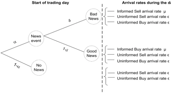
In the Glosten and Milgrom (1985) market setting, informed traders are assumed to be competitive and risk-neutral while liquidity traders buy or sell for reasons other than information on the fundamental value of the asset. Easley et al. (1996) proposed a structural model based on the sequential information model of Glosten and Milgrom (1985). Easley et al. (1996) model assume that within any trading day, the number of buyer and seller initiated trades from informed, and uninformed traders are realisations of independent Poisson distributions with mean µ and ϵ respectively. In the model a news event occur at the beginning of each trading day with probability α. With a probability δ, the news event on a "bad news day" will have a negative impact on the value of the asset. Otherwise on a "good news day", there will be a positive impact on the value of the asset.
On any given trading day liquidity traders are present in the market to either buy or sell the asset for reasons other than news. On a bad news day, informed traders expect an adverse effect on the value of the asset and are therefore likely to sell the asset. The total numbers of buy and sell orders on a bad news day are assumed to follow Poisson distributions with means ϵ and µ+ϵ respectively. On a good news day, informed traders have an incentive to buy the asset if they judge that the current asset value is under-priced and therefore expect to make gains from their private information. The total number of buy and sell orders on a good news day are Poisson with meansµ+ϵ
and ϵ respectively.
The assumption that informed traders trade on private information implies that in-formed traders are absent from the market on a day classified as a no news day. Thus
on a no news day, the total number of buyer and seller initiated trades are each Pois-son with mean ϵ. In this model, we do not observe the arrival of investors or the occurrence of a news event. However, we infer them from the observable market data. Figure 2.1 below is a representation of the information and order arrival process for the model
Fig. 2.1 Information and order arrival process in Easley et al. (1996) model
Let Bt and St denote the daily number of buyer and seller initiated trades inferred
using the Lee and Ready (1991) trade classification algorithm. The density of a buy or sell order on any given trading day t is given as follows
P (Bt, St♣Θ) =ω1 e−(µ+2ϵ)(µ+ϵ)St St! ϵBt Bt! +ω2 e−(µ+2ϵ)(µ+ϵ)Bt Bt! ϵSt St! +ω3 e−2ϵϵBt+St Bt!St! , (2.1) where Θ = (α, δ, µ, ϵ), ω1 = αδ, ω2 = α(1−δ) and ω3 = 1−α. The corresponding
joint likelihood function over a number of trading dayst = 1, . . . , T is
L(Bt, St♣Θ) = T Y t=1 ω1 e−(µ+2ϵ)(µ+ϵ)St St! ϵBt Bt! +ω2 e−(µ+2ϵ)(µ+ϵ)Bt Bt! ϵSt St! +ω3 e−2ϵϵBt+St Bt!St! . (2.2) Easley et al. (1996) estimate the model parameters by maximising equation 2.2 and
define PIN as
PIN = αµ
αµ+ 2ϵ, (2.3)
which is interpreted as the ratio of the expected number of informed trades to the total number of trades. Easley et al. (1996) suggested a minimum of 60 days worth of data to achieve stable estimates of the parameters. Due to the floating-point ex-ception, boundary solution problems of the MLE and other numerical issues of the maximum likelihood estimation reported in papers including Lei and Wu (2005), Vega (2006), Yan and Zhang (2012) and Lin and Ke (2011), we carry out the following fac-torisation of the log likelihood function
logL(Bt, St♣Θ) = T X t=1 −2ϵ+ (Bt+St) lnϵ+χ+ ln eL1−χ+eL2−χ+eL3−χ , (2.4)
prior to maximisation. In equation 2.4, we have the following:
L1 =−µ+Stln(1 + µϵ) + lnω1,
L2 =−µ+Btln(1 + µϵ) + lnω2,
L3 = lnω3, and
χ= max(L1, L2, L3).
Since the PIN is not a parameter estimate but rather a measure calculated based on the parameters any MLE optimser employed will not provide the standard error associated with the estimation of PIN. For this reason, we derive below the asymptotic variance of the PIN. Let f(Θ) be a multivariate function of the parameter set Θ. The delta method is a useful technique that can be used to derive the asymptotic variance of maximum likelihood estimators. According to the delta method (see Schervish (2012)), the asymptotic variance of f(Θ) is
V ar[f(Θ)] =∇f×X
Θ×(∇f)
′, (2.5)
where ∇f = ∂∂fΘ is a vector of the first derivates of the function f(Θ) with respect to the parameters. The term P
The PIN for the Easley et al. (1996) model can be re-written as = 1 + αµ2ϵ −1 . P IN = 1 + 2ϵ αµ −1 . (2.6)
Since news arrival is a Bernoulli variable with parameterα, informed and uninformed trade arrival intensities are poisson random variables with parametersµand ϵ respec-tively, we have α(1−nα), µn and ϵ
n as their respective asymptotic variances. The variance
of PIN in the Easley et al. (1996) model can therefore be estimated via the delta method as follows. The gradient vector is
∇P IN = ∂(P IN) ∂α ∂(P IN) ∂µ ∂(P IN) ∂ϵ = " 1 + 2ϵ αµ #−2 2ϵ α2µ 2ϵ αµ2 −2 αµ (2.7)
and the variance-covariance matrix is n−1
α(1−α) 0 0 0 µ 0 0 0 ϵ
assuming independence of parameters. Defining Ω = [1 + 2ϵ αµ]
−2 and using equation
2.5 we have V ar(P IN) = n−1Ω 2ϵ α2µ 2ϵ αµ2 −2 αµ α(1−α) 0 0 0 µ 0 0 0 ϵ 2Ωϵ α2µ 2Ωϵ αµ2 −2Ω αµ
and show that
V ar(P IN) = 4Ω 2 n ϵ α2µ2 + ϵ2µ α2µ4 + α(1−α)ϵ2 α4µ2 (2.8) We compare results of the maximisation of equation 2.4 with the estimates of the
2.3
Bayesian Inference Of Benchmark Model
Our goal is to learn about PIN and its underlying parameters from observed trans-action data. The maximum likelihood estimation approach taken in the literature assumes that the model parameters are unknown but fixed. However, in a Bayesian setting, we assume that model parameters are random and unknown. The theory behind the PIN model relates to a market maker who sets quotes and updates her knowledge about the trading behaviour of other market participants. The methodol-ogy is well suited for the estimation of PIN and its parameters since it allows for the updating of knowledge about model parameters using data from the trading process. In Bayesian inference, we express the uncertainty about the unknown model parame-ters through the rules of probability. We achieve this through the Bayes’ rule which states that the probability of the parameter set Θ given the observed data is
p(Θ♣Bt, St) = p(Θ)p(Bt, St♣Θ) p(Bt, St) ∝p(Θ)p(Bt, St♣Θ). (2.9) The denominator in 2.9, p(Bt, St) = R
p(Bt, St♣Θ)dΘ, is a normalising constant. The
term p(Θ), referred to as the prior density is not dependent on the data. It is used to express the prior knowledge and uncertainty about the model parameters before observing the data. The termp(Bt, St♣Θ), usually referred to as thelikelihood function
is the probability density function of the data conditional on the model parameters. In Bayesian inference, the primary object of interest isp(Θ♣Bt, St) which is referred to as
the posterior density. It summarises our updated knowledge of the model parameters having observed the data. It pools together information from the prior and likelihood to provide the updated information. From the posterior density, we can compute point estimates like the mean, mode and credible intervals for the model parameters. In this chapter, we employ two Bayesian Markov Chain Monte Carlo (MCMC)
meth-ods, namely the Gibbs Sampler and the Metropolis Hastings Algorithm to infer the parameters of the Easley et al. (1996) model. These methods are capable of exploring the entire support of the posterior distribution of the model parameters.
Given daily buyer and seller initiated trades Bt and St, and defining Dt as
Dt=
1, bad news day with probability ω1 =αδ
2, good news day with probability ω2 =α(1−δ)
3, no news day with probability ω3 = 1−α,
then we can write the following conditional buy and sell order distributions
St♣Dt= 1 ∼P n(µ+ϵ) Bt♣Dt = 1∼P n(ϵ) St♣Dt= 2 ∼P n(ϵ) Bt♣Dt = 2∼P n(µ+ϵ) St♣Dt= 3∼P n(ϵ) Bt♣Dt = 3∼P n(ϵ),
where P n(.)1 is the probability mass function of a Poisson random variable.
2.3.1
Method 1 : Gibbs Sampler
The latent variableDtis the process which determines the composition of traders in the
market on a daily basis. This underlying process is unobservable and hence is inferred from transaction data, as a missing data problem within the Bayesian framework. Since we do not observe trader arrival rates, good, bad or no news days, we employ the data augmentation procedure to impute these missing observations. We do this by directly sampling from the posterior distribution ofDtconditional on the available
data. In this section, we employ the theory of data augmentation to derive the density function of buy and sell trades.
1
P n(x;θ) = e−θθx
Density of buy and sell trades on a bad news day (Dt = 1)
Sell trades initiated by informed and liquidity traders on a bad news day are denoted as Si
t and Stu respectively. These are assumed to follow Poisson distributions with
meansµ and ϵrespectively. Hence the total daily seller initiated trades, St=Sti+Stu
is also Poisson with meanµ+ϵ. Given the total number of sell ordersSt, the number
of informed seller initiated tradesSi
t are binomial withSt trials and probability µ/µ+ϵ.
Uninformed seller initiated trades are determined as Su
t =St−Sti. All buyer initiated
trades on a bad news day are made by liquidity traders. The distributions of buyer and seller initiated trades are given as follows:
St♣Dt= 1∼P n(µ+ϵ), Bt♣Dt = 1∼P n(ϵ), Si t♣St, Dt= 1∼Bin St, µµ+ϵ ,
whereBin(.)2 is the probability mass function of the Binomial random variable. The
probability of a buy or sell initiated trade, on a bad news day is
f1 Bt, St, Sti,Θ =P Bt, St, Sti♣Dt= 1,Θ =P (Bt♣Dt= 1,Θ)P St, Sti♣Dt= 1,Θ =P (Bt♣Dt= 1,Θ)P Sti♣St, Dt= 1,Θ P (St♣Dt= 1,Θ) =e −ϵϵBt Bt! St Si t ! µ µ+ϵ Sti ϵ µ+ϵ St−Sit(µ+ϵ)Ste−(µ+ϵ) St! = St Si t ! e−(µ+2ϵ)ϵBt Bt!St! µSi tϵSt−Sti =e −µµSi t Si t! e−ϵϵBt Bt! e−ϵϵSt−Si t (St−Sti)! . (2.10)
Density of buy and sell trades on a good news day (Dt= 2)
The total number of buyer initiated tradesBt on a good news day comprises of buyer
initiated trades Bi
t and Btu made by informed and uninformed traders respectively.
2
Bn(n;r;θ) = nθ
These buyer initiated trades are assumed to be Poisson with meanµandϵ, henceBtis
Poisson withµ+ϵ. Conditional on the total daily buyer initiated tradesBt, the number
of buyer initiated trades from informed trades Bi
t are binomial distributions with Bt
trials and probabilityµ/µ+ϵ. The uninformed buyer initiated trade is calculated asBu
t =
Bt−Bit. All seller initiated trades on a good news day are made by liquidity traders.
Thus we have Bt♣Dt = 2 ∼ P n(µ+ϵ), Bti♣Bt, Dt = 2 ∼ Bin
Bt,µµ+ϵ
and St♣Dt =
2∼P n(ϵ) as the distributions of the buyer and seller initiated trades on a good news day. The probability density of a buy and sell trades, on a good news day is given below f2 Bt, St, Bti,Θ =P Bt, Bt, Bti♣Dt= 2,Θ =P (St♣Dt = 2,Θ)P Bi t♣Bt, Dt= 2,Θ P(Bt♣Dt= 2,Θ) =e −ϵϵSt St! Bt Bi t ! µ µ+ϵ Bit ϵ µ+ϵ Bt−Bit(µ+ϵ)Bte−(µ+ϵ) Bt! =e −µµBi t Bi t! e−ϵϵSt St! e−ϵϵBt−Bi t (Bt−Bti)! . (2.11)
Density of buy and sell trades on a no news day (Dt= 3)
Easley et al. (1996) assume that informed traders do not trade on no news days. Hence the total number of buyer and seller initiated trades are made solely by liquidity traders. The arrivals are independent Poisson distributions Bt♣Dt = 3 ∼ P n(ϵ) and
St♣Dt= 3∼P n(ϵ) respectively. The probability density of a buyer or seller initiated
trade on a no news day is
f3(Bt, St,Θ) =P (Bt, St♣Dt= 3,Θ) =P (St♣Dt= 3,Θ)P(Bt♣Θ)P (Bt♣Dt= 3,Θ) =e −2ϵϵBt+St Bt!St! . (2.12)
The Poisson mixture assumption underlying the model can be seen in equations 2.10, 2.11 and 2.12. We define the following indicator random variable dt,j = 1¶Dt=j♦, for
j = 1,2,3. Putting equations 2.10, 2.11 and 2.12 together, the density function of buy and sell orders is
P (Bt, St♣Θ, Dt) = " f1(Bt, St,Θ) #dt,1" f2(Bt, St,Θ) #dt,2" f3(Bt, St,Θ) #dt,3 = " e−µµSi t Si t! e−ϵϵBt Bt! e−ϵϵSt−Si t (St−Sti)! #dt,1" e−µµBi t Bi t! e−ϵϵSt St! e−ϵϵBt−Bi t (Bt−Bti)! #dt,2" e−2ϵϵBt+St Bt!St! #dt,3 . (2.13)
Posterior Density And Full Conditional Distributions
Since the probability of news arrival α and its effect δ are both positive values that lie strictly in the interval (0, 1) we choose beta distributions for their prior distribu-tions. Likewise we choose gamma prior distributions for the positive parameters µ
and ϵ. Finally, we choose a Dirichlet prior for the type of day classifier Dt. The prior
distributions for parameter set Θ = (α, δ, µ, ϵ, Dt) are
P(α♣ρ, φ) = 1 Beta(ρ,ε)α ρ−1(1−α)φ−1 , P(δ♣ν, τ) = Beta1(ν,τ)δν−1(1−δ)τ−1 , P(µ♣γ0, β0) = βγ0 0 Γ(γ0)µ γ0−1e−β0µ. P(ϵ♣γ1, β1) = βγ1 1 Γ(β1)λ γ1−1 s e−β1λs, Dt∼Dirichlet(π1, π2, π3) and
With these conjugate prior distributions the resulting posterior distributions will have kernels which are proportional to standard probability distributions. The Gibbs Sampler can then be easily applied to sample from the posterior distributions. We set each of the hyper-parameters ρ, φ, ν, τ, γ0, γ1, β0, β1 to the value 1 and
π1 = π2 = π3 = 1/3. This means that α and δ can take on any number between
zero and one with probability 1. The priors for ϵ and µ are informative since their respective means and variances are equal to 1. The hyper-parameter choices will have little influence on the parameter estimates since after a large enough iterations of the
Gibbs Sampler, the markov chain converges to the true parameter. From Bayes’ theo-rem, the posterior density for the parameter set Θ = (α, δ, µ, ϵ) is proportional to the product of the likelihood and prior. This is given as
P (Θ♣Bt, St)∝P (Θ) T Y t=1 " P(Bt, St♣Dt,Θ)P (Dt♣Θ) # =µγ0−1e−β0µϵγ1−1e−β1ϵαρ−1(1−α)φ−1δν−1(1−δ)τ−1 " (αδ)T1(α(1−δ))T2(1−α)T3 # × T Y t=1 " e−µµSi t Si t! e−ϵϵBt Bt! e−ϵϵSt−Si t (St−Sti)! #dt,1" e−µµBi t Bi t! e−ϵϵSt St! e−ϵϵBt−Bi t (Bt−Bti)! #dt,2" e−2ϵϵBt+St Bt!St! #dt,3 . (2.14) The full conditional distributions of the parameters Θ = (α, δ, µ, ϵ) are needed for the Gibbs Sampler. From equation 2.14 we have the following full conditional densities for the parameters
µ∼ Ga γ0+ T X t=1 [(Sti)dt,1 + (Bi t)dt,2], T1+T2+β0 ! (2.15a) δ ∼ Be ν+T1, T2+τ (2.15b) α∼ Be ρ+T1+T2, T3+φ (2.15c) ϵ∼ Ga γ1+ T X t=1 [Bd1 t +Std1 −(Sti)d1+Std2 +Btd2−(Bit)d2 +Btd3 +Std3], 2T+β1 , (2.15d)
where T1, T2 and T3 are the number of good, bad and no news days respectively such
that T =T1+T2+T3.
Gibbs Sampling Procedure
The algorithm recursively draw samples from the full conditional posterior distribu-tions where the most recent values of the parameters are used in the simulation. The procedure is as follows:
• Choose an arbitrary initial type of day (good, bad and no news day) classification for the (Bt, St). Denote the initial classification as Dt(0).
• Set initial values for the parameter set Θ. Denote it as Θ(0)=α(0), δ(0), ϵ(0), µ(0).
• Repeat for k = 1 to Gsweeps
– Sample Bti(k)♣D (k−1) t ∼Bin Bt, µ (k−1) µ(k−1)+ϵ(k−1) , t= 1, . . . , T – Sample Sti(k)♣D (k−1) t ∼Bin St, µ (k−1) µ(k−1)+ϵ(k−1) , t= 1, . . . , T – Update µ(k)♣α(k−1), ϵ(k−1), δ(k−1), Bi(k) t , S i(k) t – Update α(k)♣µ(k), ϵ(k−1), δ(k−1), Bi(k) t , S i(k) t – Update ϵ(k)♣µ(k), α(k), δ(k−1), Bi(k) t , S i(k) t – Update δ(k)♣µ(k), α(k), ϵ(k), Bi(k) t , S i(k) t – Compute L1 = logω(1k)− µ(k)+ 2ϵ(k)+B tlogϵ(k)+Stlog µ(k)+ϵ(k) – Compute L2 = logω(2k)− µ(k)+ 2ϵ(k)+S tlogϵ(k)+Btlog ϵ(k)+µ(k)
– Compute L3 = logω(3k)−2ϵ(k)+ (St+Bt) logϵ(k)
– compute χ= max (L1, L2, L3) – Compute p1 = e L1−χ 3 P j=1 eLj−χ , p2 = e L2−χ 3 P j=1 eLj−χ and p3 = e L3−χ 3 P j=1 eLj−χ
– UpdateDt(k), the classification of (Bt, St) by sampling from the multinomial
distribution with probability
p1, p2, p3
,
wherep1,p2 andp3 are the probabilities that at the beginning of the trading day there
2.3.2
Method 2: Metropolis-Hastings Algorithm
The Metropolis Hastings algorithm is a MCMC algorithm for drawing samples from the posterior distribution of high dimensional parameter and intractable complex model problems. The algorithm is used to draw samples of the parameter set Θ′ =
(α′, δ′, µ′, ϵ′) from an approximating distribution which has the same support as the
posterior density. The approximating distribution which we denote as q
Θ′,Θ(t−1)
is referred to as a proposal density.
The algorithm involves two basic steps. Firstly a draw from the proposal density is obtained. Secondly, the draw is either retained or rejected. Details of the algorithm are summarised as follows
1. Initialise the algorithm with values Θ(0) from the parameter space of Θ.
2. At iterationt, a draw Θ′ is taken from the proposal densityqΘ′,Θ(t−1)where
Θ(t−1) is the value of the parameter in the previous step.
3. The new draw is accepted with probability min
1,π(Θπ(Θ(t−′)1)q(Θ)q(Θ(t−′,1)Θ,(Θt−′)1))
, where
π(Θ) is the posterior density.
4. Steps 2 and 3 are repeated for a large number of iterations.
Now we proceed to derive the posterior density needed for the sampling. For easy com-parison of results we use the same conjugate prior distributions and hyper-parameters for α, δ, µ, ϵ and Dt which were chosen for the Gibbs Sampler. The choices as
indi-cated earlier is to ensure that we have the draws not falling on the boundary of the respective parameter space. The joint posterior density of buyer and seller initiated
trades is given as P (Θ, Dt♣Bt, St)∝P(α♣ρ, φ)P(δ♣ν, τ)P(µ♣γ0, β0)P(ϵ♣γ1, β1) × T Y t=1 αδe−(µ+2ϵ)(µ+ϵ)St ϵBt +α(1−δ)e−(µ+2ϵ)(µ+ϵ)Bt ϵSt + (1−α)e−2ϵϵBt+St =αρ−1(1−α)φ−1 δν−1(1−δ)τ−1 µγ0−1e−β0µϵγ1−1e−γ1ϵ × T Y t=1 αδe−(µ+2ϵ)(µ+ϵ)St ϵBt +α(1−δ)e−(µ+2ϵ)(µ+ϵ)Bt ϵSt + (1−α)e−2ϵϵBt+St , (2.16) Taking logarithm of the posterior density in equation 2.16 we have
ln (P (Θ♣Bt, St)) = T X t=1 ln eL1−χ+eL2−χ+eL3−χ + T X t=1 −2ϵ+ (Bt+St) ln(ϵ) +χ +(γ0−1) ln (µ)−β0µ+ (γ1−1) ln (ϵ)−β1ϵ+ (ρ−1) ln (α) +(φ−1) ln (α) + (ν−1) ln (δ) + (τ −1) ln (δ), where L1 =−µ+Stln(1 + µϵ) + ln(αδ), L2 =−µ+Btln(1 + µϵ) + ln[α(1−δ)], L3 = ln(1−α) and χ= max(L1, L2, L3).
We use a random walk Metropolis-Hastings algorithm with standard Gaussian innova-tions to draw samples from the posterior distribution of the parameters. The random walk proposal is Θ′ = Θ(t−1)+ε, whereε
t ∼ N(0, ξ). Since the random walk proposal
density is symmetric, the acceptance probability simplifies to
acceptance probability = min ( 1,P(Bt, St♣Θ ′)P(Θ′) P(Bt, St♣Θ)P(Θ) ) . (2.17)
We start off the Bayesian estimation with arbitrary initial values for algorithm. The Markov chain initially explores regions of the parameter space around the initial values and finally converge to most probably parameter space. However, including samples around the initial values in the posterior mean calculation can produce substantial bias in the mean estimate. The practice of discarding an initial portion of a Markov chain sample so that the effect of initial values on the posterior inference is minimised is known as burn-in period. To improve the convergence of the Markov chain, we implemented the Adaptive Metropolis-Hastings algorithm (AMH) developed by Haario et al. (2001) which we briefly describe below.
The Haario et al. (2001) AMH algorithm
1. For each element of the parameter set Θ = (α, δ, µ, ϵ), set initial values Θ(0),ξ(0),
MCMC samples G, burnin n0, and t0
2. For t= 1,2, . . . do
3. Sample Θ′ = Θ(t)+ε
t where εt ∼ N
0, ξ(t)
4. Accept the next iterate Θ(t+1)= Θ′ with probability given in equation 2.17
5. Compute ξ(t+1) = ξ(0) if t≤t 0, sd×ϕ×Id+ts−1d × " t P j=1Θ (j)Θ(j)T − t P j=1 Θ(j) t P j=1 Θ(j) T t # , if t > t0
where ϕ is a small positive constant, Id is a d-dimensional identity matrix and
sd is a scale parameter
6. end for
7. Collect samples Θ(n0+1), . . . ,Θ(n0+G)
The scaling parameter sd = 2.42/d where d is the dimension of Θ. This value was
proposed in Gelman et al. (1996) to optimise the mixing properties of the Metropolis algorithm.
2.4
Extension Of The Benchmark PIN Model
Buyer and seller initiated trades made by liquidity traders in Easley et al. (1996) were assumed to be Poisson with the same arrival rates. Easley et al. (2002) relaxed this assumption since in reality, liquidity traders who want to buy or sell an asset do not arrive at the market at the same rate. In this model the means of the liquidity trader buyer and seller initiated trade distributions are λb and λs respectively. All other
assumptions in the previous model remain unchanged.
Since order arrivals on a bad news day are assumed to follow independent Poisson distributions, the total number of buyer and seller initiated trades on a bad news day are Poisson with means λb and µ+λs respectively. On a good news day, the total
number of buyer and seller initiated trades are also Poisson with parameters µ+λb
and λs respectively. Likewise, on a no news day the total number of buyer and seller
initiated trades are Poisson with parametersλb and λs respectively.
Figure 2.2 is a representation of the information and order arrival process for the model.