Software reliability prediction using neural network

(1)

Software Reliability Prediction Using

Neural Network

Thesis submitted in partial fulfillment of

the requirements for the degree of

Bachelor of Technology in Computer Science and Engineering

by

Rosalin Maharana

Roll No-110CS0303

under the guidance of

Dr. Durga Prasad Mohapatra

Department of Computer Science and Engineering National Institute of Technology Rourkela

Rourkela-769008, Odisha, India May 2014

(2)

Certificate

This is to certify that the work in the thesis entitled “Software Reliability Prediction

Using Neural Network” by Rosalin Maharana is a record of an original research work carried out under my supervision and guidance in partial fulfillment of the requirements for the award of the degree of Bachelor of Technology in Computer Science. The thesis fulfills all requirements as per the regulations of this Institute and has reached the standard needed for submission. Neither this thesis nor any part of it has been submitted for any degree or academic award elsewhere.

Dr. Durga Prasad Mohapatra

Department of Computer Science and Engineering National Institute of Technology Rourkela

Department of Computer Science and Engineering

National Institute of Technology Rourkela

(3)

Acknowledgement

On the submission of the Thesis report, we would like to extend our gratitude and sincere thanks to our supervisor Dr. D. P. Mohapatra, for his constant motivation and support during the course of this work in the last one year. We truly appreciate and value his esteemed guidance and encouragement from the beginning to the end of this thesis. He has been our source of inspiration throughout the thesis work and without his invaluable advice and assistance it would not have been possible for us to complete this thesis.

We would also like to give our most sincere thanks to Dr. S. K. Rath, Head of the Department of Computer Science and Engineering for his support during our work. A special acknowledgement goes to Mr Manmath Kumar Bhuyan, a PhD scholar for his guidance throughout the thesis. We would also like to express our thanks to all who extended their unlimited help to us during our project work and its subsequent documentation.

Last but not least we would like to thank all professors and members of the department of Computer Science and Engineering, NIT Rourkela for their generous help in various ways in completion of this thesis.Furthermore, we would like to take the name of our parents and God who directly or indirectly encouraged and motivated us during this dissertation.

(4)

Declaration

I hereby declare that all the work contained in this report is my own work

unless otherwise acknowledged. Also, all of my work has not been previously

submitted for any academic degree. All sources of quoted information have

been acknowledged by means of appropriate references.

Rosalin Maharana

NIT Rourkela

(5)

Abstract

Software engineering is incomplete without Software reliability prediction. For characterising any software product quality quantitatively during phase of testing, the most important factor is software reliability assessment. Many analytical models were being proposed over the years for assessing the reliability of a software system and for modeling the growth trends of software reliability with different capabilities of prediction at different testing phases. But it is needed for developing such a single model which can be applicable for a relatively better prediction in all conditions and situations. For this the Neural Network (NN) model approach is introduced. In this thesis report the applicability of the models based on NN for better reliability prediction in a real environment is described and a method of assessment of growth of software reliability using NN model is presented. Mainly two types of NNs are used here. One is feed forward neural network and another is recurrent neural network. For modeling both networks, back propagation learning algorithm is implemented and the related network architecture issues, data representation methods and some unreal assumptions associated with software reliability models are discussed. Different datasets containing software failures are applied to the proposed models. These datasets are obtained from several software projects. Then it is observed that the results obtained indicate a significant improvement in performance by using neural network models over conventional statistical models based on non homogeneous Poisson process.

(6)

i

List of Figures

Figure 2.1: A simple model of artificial neuron---9

Figure 3.1: Flowchart for back propagation algorithm---12

Figure 3.2: A sample feed forward network---13

Figure 3.3: A sample recurrent neural network---15

Figure 4.1: Performance of FFNN for Dataset1---22

Figure 4.2: Snapshot of performance of FFNN for Dataset1---23

Figure 4.3: Performance of FFNN for Dataset2--- 24

Figure 4.9: Performance of RNN for Dataset1---30

List of Tables

Table 4.1: Table of different software failure datasets used---17

Table 4.2: Feed forward neural network model results ---20

Table 4.3: Recurrent neural network model results---20

Table 4.4: Comparison with analytical models---21

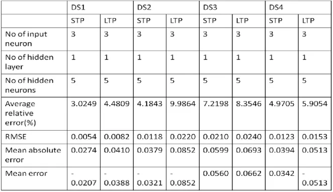
Table 4.5: Comparison between LTP and STP for feed forward neural network---21

(8)

1

Chapter 1 Introduction

Software is playing an ever-increasing role in our real time systems. Therefore there has been a gradual growth of concern over quality of software products and reliability has become a main concern from both software user’s point of view and software developers’ point of view. Also the rapid growth of software products in size and complexity has drawn the attention of researchers to be more focused on quality assessment by the estimation of the time of software testing period quantitatively to avoid any unwanted and unforeseen situation during operational phase. In this thesis report the applicability of neural network models for better reliability prediction in real environment are explored empirically and an assessment method of growth of software reliability using artificial neural network (ANN) mode is presented.

Artificial neural networks are generally known as “Neural Networks” and act in a way similar to the human brain. Non linearity and complexity of the brain is very high and behaves like a parallel computer. It has the ability for organizing its structural constituents known as neurons; hence it performs certain computation very quickly than the fastest computer present on earth. The brain structure is very intense and it builds up its own rules through experiences. Experiences are built up over time with the development of the human brain through many stages. A developing neuron is as similar as a plastic brain. To adapt with the surrounding environment the developing nervous system has the property of plasticity. Plasticity appears to be essential to the functioning of neurons as information processing units in the human brain. Similarly this same thing happens with neural networks made up of artificial neurons. A neural network is a machine that is designed to model the way in which the brain performs a particular task. To achieve good performance, neural networks should have a massive interconnection of simple computing cells referred to as

(9)

2

“neurons” or “processing units”. Neural networks perform essential computations through a process of learning.

Thus a neural network consists of simple processing units and big parallel distributed processors. The ability of storing experiential data and making it available for use comes naturally to it. Artificial neural network do not approach the complexity of the brain. It is similar to brain in two ways: 1.A learning process is used to acquire knowledge from its surrounding by the network. 2. The acquired knowledge is stored by the interneuron connection strengths known as synaptic weights. The procedure used to perform the process of learning is called learning algorithm. Function of learning algorithm is to modify the synaptic weights of the networks in an orderly manner in order to attain a desired design objective.

1.1 Motivation of Our Work

The software market is very competitive in this dynamic world. Software industries attempt to release software to grab the market as soon as it is ready. Now it is a challenge for software developers to rapidly design, implement, test, and maintain complex hardware or software systems as per the demands of the users. Also it is a challenge for software companies to deliver good quality and error free software in right time. The impact of the failures produces severe consequences such as environmental impact, inconvenience, economical losses, loss of human life etc. Needless to say, the reliability of computer systems has become a major concern for our society. Software reliability is an important facet of software quality characteristic. Many researchers have used neural networks to predict software reliability. Different neural networks with different learning methods also have been modelled. It is also observed that connectionist models perform better than the previous parametric models. Prediction of software reliability using computational intelligence (CI) can be very accurate and significant compared to traditional statistical methods. CI can offer promising approaches to software reliability prediction and modeling.

(10)

3

With this motivation, we implemented different neural network models with different learning algorithms and compared their performance results for software reliability prediction with the statistical methods and observed that neural networks perform better than the analytical models. The details of the work are described in the next chapter.

1.2 Objective of Our Work

The main objective of this research work is to implement different connectionist models with different learning regimes. Different datasets containing software failures are applied to the proposed models. These datasets are obtained from several software projects. Then different issues related to method of data representation, some unrealistic assumptions incorporated with software reliability models, and network architecture are discussed.

We have tried to implement the feed forward neural network architecture first with back propagation learning method for reliability prediction. As no work is done regarding the implementation of recurrent neural network with back propagation algorithm till now, so mainly our objective is to implement recurrent neural network architecture with back propagation learning algorithm. Followings are the key points of our implementation.

 Feed Forward Neural Network with one hidden layer and multiple hidden layer along with back propagation learning method

 Recurrent Neural Network with back propagation learning method

 Long term predictability and Short term predictability of feed forward neural networks

 Evaluation of effectiveness of the above proposed models by using different performance parameters

(11)

4

1.3 Organisation of The Thesis

The rest of this thesis report is organised into chapters as follows.

 Chapter 2 describes about the related work done and gives an overall literature review.

 Chapter 3 provides the background concepts used in the remaining part of the thesis. Some theoretical concepts regarding software reliability measures, artificial neural network and back propagation learning algorithm are described. Some basic concepts of feed forward and recurrent neural network are presented.

 Chapter 4 provides a brief review and implementation details of the project work.

 Chapter 5 describes the experimental results of the implemented network models and their performance results.

 Chapter 6 concludes the thesis report with a summary and possible future extension of this work.

1.4 Literature Review

Artificial Neural Network (ANN) is a powerful technique for Software Reliability Prediction.

Werbos [9] proposed back-propagation learning as an alternative to regression technique to identify sources of forecast in uncertainty in a recent gas market model. Thus it can be concluded that neural network models are very useful for regression techniques of forecasting in uncertainty of any data.

Shadmehr et al. [10] estimated model parameters of pharmacokinetics system using feed forward multilayered network and predicted the noise resides in the measured data sample. The authors compared the results with that of the optimal

(12)

5

Bayesian estimator and found the performance was better than the maximum likelihood estimator [11].

The ANN tools and feed forward network using back propagation algorithm are applied for reliability and software quality prediction [12–14]. The authors developed a connectionist model and took failure data set as input to produce reliability as output. These papers describe network architecture, method of data representation and some unrealistic assumptions associated with software reliability models.

Karunanithi et al. [15] predicted software reliability using feed forward network and recurrent network. The authors compared the result with 14 different literature representative data sets and suggested that neural network produced better predictive accuracy compared to analytical models at end-point predictions.

Sitte [16] analyzed two methods for software reliability prediction: 1) neural networks and 2) parametric recalibration models. These approaches differentiate the neural networks and parametric recalibration models in the context of software reliability prediction and conclude that neural networks are much simpler and better predictors.

Tian et al. [7] predicted software reliability using recurrent neural network. Bayesian regularization is applied to train the network. The authors commented that their proposed approach produced less average relative prediction error than well known prediction techniques.

RajKiran et al. [17] implemented the use of wavelet neural networks (WNN) to predict software reliability. In this paper, the authors employed two kinds of wavelets i.e. Morlet wavelet and Gaussian wavelet as transfer functions. They made a comparison on test data with multiple linear regression (MLR), multivariate adaptive regression splines (MARS), back-propagation trained neural network (BPNN) and threshold accepting trained neural network (TANN), pi-sigma network (PSN), general regression neural network (GRNN) and found that its performance is better than others.

(13)

6

Lo [18] designed a model for software reliability prediction using artificial neural networks. This approach examines several conventional software reliability growth models without assuming some unrealistic things.

Fuzzy Wavelet Neural Network (FWNN) is used for phase space reconstruction technology and for software reliability prediction [19]. In this work, the network architecture is designed easily by taking the failure data as input.

(14)

7

Chapter 2 Background

2.1 Software Reliability

The probability that a software will perform a required function under stated conditions for a specified period of time is known as software reliability. Software reliability assessment is a very vital factor to characterise the quality of any software product quantitatively during testing phase.

Software Reliability Measures

 Failure Rate: It is the rate of occurrence of failures. It also represents number of failures in specified period of time.

 Mean Time Between Failures (MTBF): It is the average time between failures. No of hours taken to pass before a failure occurs is the MTBF. It is the inverse of failure rate.

 Reliability: The probability that an item will perform a required function without failure under the stated conditions for a specified period of time is called reliability. It takes into account the mission time.

 Availability: The probability that an item is in operable state at any time is called availability. It accounts for repairs and down time.

Software Reliability Growth Models

It includes two types of models

 Parametric models

 Nonparametric models

Parametric models are based on non homogeneous Poisson process. Neural network is non parametric model and based on statistical failure data. Nonparametric models are more flexible.

(15)

8

Different Reliability Metrics

 Failure rate

 Next time to failure

 Time between failures

 Cumulative failures detected

2.2 Artificial Neural Network

 It is can be defined as a system where data can be processed through a number of nodes similar to neurons in brain.

 Each node is assigned with a function and it determines the node output with the help of some parameters available locally to it for a set of given input.

 By adjusting weight of these parameters the node function can be altered as intended.

2.3 Neural Network Modeling

 Like a brain, a neural network also performs in similar fashion. It has some learning mechanism designed within it for modelling the reliability.

 A number of neurons constitute NN which are simple processing elements. These neurons are connected to each other directly through communications links associated with some weight.

 Supervised learning method is used to train the NN with a series of sample input and to compare the responses overall for the pre specified period of time with the expected sample output.

 The training procedure is carried out until expected and convincing responses are provided by the network. The neurons are arranged layer by layer and the connection patterns within and in-between layers make the network architecture.

 The network can be either single-layered or multi-layered; layers of interconnected links between the neuron slabs determine it.

(16)

9

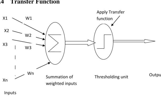
2.4 Transfer Function

Figure 2.1: A simple model of artificial neuron

Let I=input to the neural network

Where Then Y=F (I)

where Y is the output of the neural network and F is the transfer function.

Hyperbolic Tangent Transfer Function

Y=F ( I)=

-

Y varies between -1 and +1.

| | | | X2 X1 X3 W1 W2 Wn W3 Summation of weighted inputs Thresholding unit Xn Inputs Output Apply Transfer function

(17)

10

Log Sigmoid Transfer Function

Y=F ( I)=

Y varies between 0 and +1.

Both log sigmoid and hyperbolic tangent functions are continuous. In this thesis report we have used log sigmoid as transfer function.

(18)

11

Chapter 3 Work Details

We have implemented feed forward neural network and recurrent neural network with back propagation learning algorithm.

3.1 Back Propagation Learning Algorithm

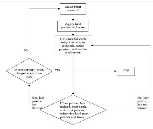
Algorithm:

1. Initialize the weights 2. Repeat

3. For each training pattern 4. Train on that pattern

5. Find error for each pattern and mean square error for total no of patterns

6. Update the connecting weights by calculating errors layer by layer backward

7. End

(19)

12

Figure 3.4: Flowchart for back propagation algorithm

3.2 Approach for Feed Forward Neural Network

• Here Back Propagation Learning rule is applied to a feed forward network.

• The basic feed forward neural network architecture comprises in two steps.

– 1) feed forward NN

– 2) back propagation

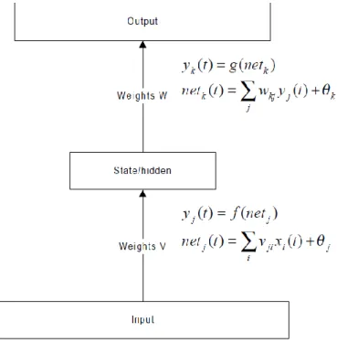
• Here the input vector is propagated through a weight layer. It is combined with the previous state activation as it depicted in next Figure 3.2.

• The conventional feed-forward neural network consists of two-layered network. The network comprises of two steps mapping.

y(t) = G(F(x(t)) ………...(1)

• The back-propagation learning techniques are used in the above equation 1 to update the weights of the network (F and G) for training the feed forward back propagation network. The operation is restricted in this paper to (“hidden/state” layer and “output” layer).

(20)

13

• The input vector ’x’ is propagated with a layer associated with weight V as depicted in equation 3.

yj(t) = f(netj)(t) ---(2)

n

net_j(t) = Σ (v_ji)(x_i(t) )+ θ_i---(3) i

where n is the number of inputs nodes, θ_i is a bias and f is an activation function.

• The output of the network is calculated by state and weight W associated with that output layer.

y_k(t) = g(net_k(t))--- (4) m

g(net_k(t)) =Σ y_j(t)w_kj+ θ_k--- (5) j

where m is the number of states or ‘hidden’ nodes, θ_k is a bias and g is an activation function.

Here sigmoid function is taken as activation function.

(21)

14

3.3 Approach for Recurrent Neural Network

• Here Back Propagation Learning rule is applied to a recurrent network.

• The basic recurrent neural network architecture comprise in two steps.

– 1) feed forward NN

– 2) back propagation with recurrent.

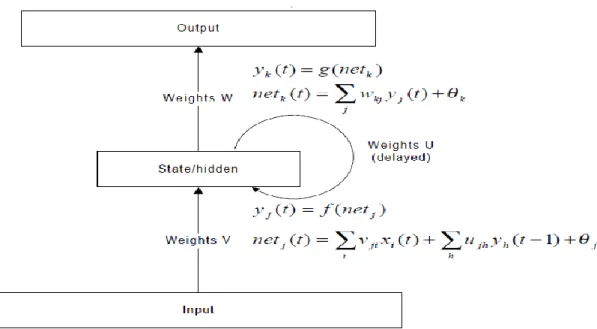
• Here the input vector is propagated through a weight layer. It is combined with the previous state activation through an additional recurrent weight layer, R as it depicted in next Figure 3.3.

• The conventional feed-forward neural network consists of two-layered network. The network comprises of two steps mapping

y(t) = G(F(x(t)) ………..(1)

• The back-propagation learning techniques are used in the above equation 1 to update the weights of the network (F and G) for training the Recurrent Back Propagation Network. The operation is restricted in this paper to (“hidden/state” layer and “output” layer).

• The input vector ’x’ is propagated with a layer associated with weight V and combined with previous state activation associated with recurrent weight U as depicted in equation 3.

y_j(t) = f(net_j)(t) ---(2) n m

netj(t) = Σ (vji)(xi(t) )+Σ (ujh)(yh(t − 1) )+ θi---(3)

i h

where n is the number of inputs nodes, θ_i is a bias, m is the number of states or ‘hidden’ nodes, and f is an activation function.

• The output of the network is calculated by state and weight W associated with that output layer.

yk(t) = g(netk(t))--- (4)

m

g(netk(t)) =Σ yj(t)wkj + θk--- (5)

j

(22)

15

Here sigmoid function is taken as activation function.

(23)

16

Chapter 4 Implementation & Results

4.1 Implementation setup

 The FFNN and RNN with back propagation learning algorithm is implemented using MATLAB 7.10.0.499.

 In our prediction experiment, failure data during system testing phase of various projects collected at Bell Tele-phone Laboratories, Cyber Security and Information Systems In-formation Analysis Centre(CSIAC) by John D. Musa are considered.

 CSIAC provides software failure datasets in order to support the project manager to monitor testing, estimating the project schedule, and helping the researchers to evaluate the reliability model.

 The data set consists of

o Failure Number

o Failure Interval Lengths/Time Between Failures (TBF) in CPU secs

o Day of Failure of software project

 We have taken 5 numbers of application software testing data set for demonstration of predictive performance and prediction accuracy as shown in Figure 5.1.

 70% of each dataset is used for training the model and the rest failure data is used for validating the model.

(24)

17

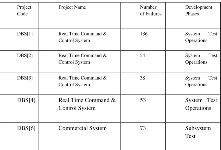
Table 4.1: Table of different software failure datasets used

Project Code

Project Name Number

of Failures

Development Phases

DBS[1] Real Time Command &

Control System

136 System Test

Operations

Control System

54 System Test

Operations

Control System

38 System Test

Operations

DBS[4] Real Time Command & Control System

53 System Test Operations

DBS[6] Commercial System 73 Subsystem Test

• For FFNN proposed model,

– Cumulative Execution time is taken as input

– No of Cumulative Failures is taken as output

– Both cumulative execution time and no of cumulative failures are normalized in the range 0 to 1.

– Graph is plotted with cumulative execution time in X-axis and no of cumulative failures in y-axis.

• For RNN proposed model

– Cumulative execution time for nth failure is taken as input

(25)

18

– Graph is plotted with no of failure taken in X-axis and cumulative execution time in y-axis.

– Cumulative execution time is normalized in the range 0 to 1.

4.2 Different Performance Measures

• The following performance measures are being used to validate the proposed models:

– Relative Error(%): REi = ( | (Pi-Ai ) / Ai | ) * 100

n

– Average Relative Error(%): 1/n ∑ REi

n 2

– Root Mean Squared Error: RMSE = √ [ ( ∑ (P_i-A_i) ) / n ] n

– Mean Absolute Error: [ ∑ | Pi-Ai | ] / n

n – Mean Error: [ ∑ (Pi-Ai) ] / n where P_i=Predicted Value A_i=Actual Value n=total no of observations/patterns

4.3 Prediction Types

• Neural Networks can predict software reliability in two ways:

– Long Term Prediction

(26)

19

Short term prediction (STP)

Suppose we have a software failure dataset having the following format. Cumulative

execution time No of failures

t1 x1 t2 x2 t3 x3 | | tk xk t(k+1) x(k+1) | | tn xn t(n+1) x(n+1)

We can interpret no of failures as a function of cumulative execution time . Suppose y is the function, then y can be written as y(t)=x

• Then a neural network can be modeled by with 3 layers taking k input neurons in input layer, 1 output neuron in output layer and a hidden layer.

• Taking y(t1),y(t2),y(t3)…y(tk) as inputs to the neural network and Predicting y’(t(k+1)) as output(where y(t(k+1)) is taken as target value) is known as short term prediction or 1-step ahead prediction .

Long term prediction(LTP)

Considering the neural network model as explained in previous section,

 y(t1),y(t2),y(t3)…y(tk) are taken as inputs to the neural network and y’(t(k+1)) is predicted as output(where y(t(k+1)) is taken as target value).

 Then y(t2),y(t3),y(t4)…y’(t(k+1)) are taken as inputs to the neural network and y’(t(k+2)) is predicted as output(where y(t(k+2)) is taken as target value).

 Continuing like this up to nth pattern is known as long term prediction or n-step ahead prediction.

(27)

20

4.4 Results and Discussion

Different dataset are taken and results are shown in the following tables and

figures.

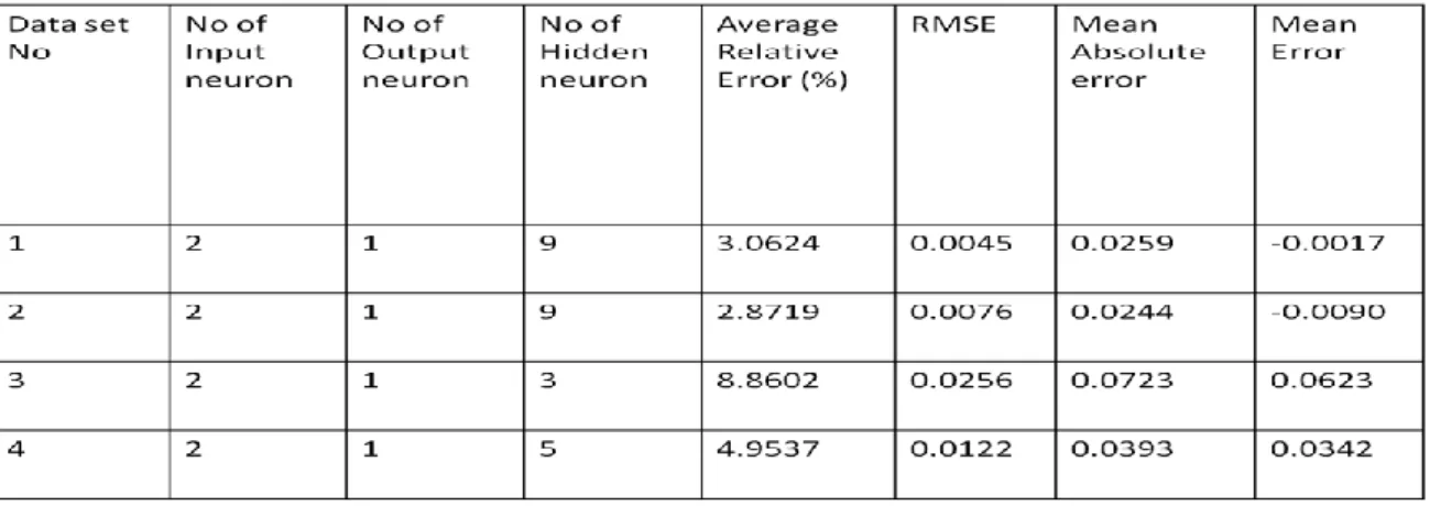
Table 4.2: Feed forward neural network model results

(28)

21

Table 4.4: Comparison with analytical models

(29)

22

4.5 Graphs and Screenshots

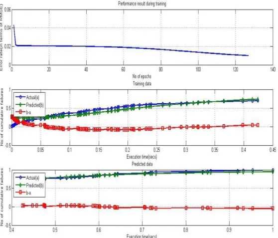
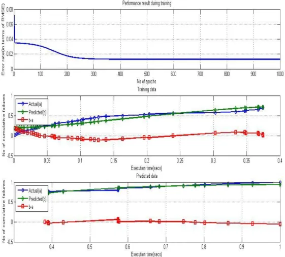
Figure 4.1: Performance of FFNN for Dataset1

In the above figure, plots for feed forward neural networks are shown. The first graph is the plot between number of epochs vs. error rate in terms of RMSE during training. It shows how the error rate gradually decreases with the no of epochs by the use of back propagation learning. The second and third graph is the plot between cumulative execution time vs. no of cumulative failures for Dataset1. Second graph is plotted for the training period and third graph is plotted for the prediction period. In both second and third graph blue colour line represents actual data, green colour line represents predicted data and red colour line represents difference between predicted data and actual data.

(30)

23

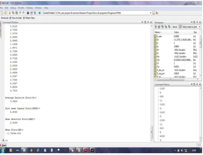
Figure 4.2: Snapshot of performance of FFNN for Dataset 1

In the above figure, the snapshot of different performance measure values using FFNN for Dataset1 is shown.

(31)

24

(32)

25

Figure 4.4: Snapshot of performance of FFNN for Dataset2

(33)

26

(34)

27

(35)

28

(36)

29

(37)

30

Figure 4.9: Performance of RNN for Dataset1

In the above figure, plots for recurrent neural networks are shown. The upper two graphs are the plot between no of cumulative failures vs. cumulative execution time for Dataset1. Upper left graph is plotted for the training period and upper right graph is plotted for the prediction period. In both upper graphs red colour line represents actual data; blue colour line represents predicted data. In the lower two graphs red colour line represents difference between predicted data and actual data.

(38)

31

(39)

32

(40)

33

Chapter 5 Conclusion and Future Work

5.1 Conclusion

We have successfully implemented the feed forward and recurrent neural network with back propagation learning algorithm. The observations conclude that neural network model performs better in terms of less error in prediction as compared to existing analytical models and hence it is a better alternative to do software reliability test using neural network. However it can be seen from the figures that the NN method proposed in this paper using back propagation algorithm provides a good fit than analytical models.As the connection weights are randomly initialized, thus the neural network gives different results for the same datasets and thus the performance of the network varies. The usefulness of a Neural Network method is dependent on the nature of dataset up to a greater extent. In most cases STP gives better result than LTP. Neural Network model gives better result for larger datasets than smaller datasets.These models are easily compatible with different smooth trend data set and projects. We have implemented the program in MATLAB. But the programs can be implemented in other languages such as Java, Python etc.

(41)

34

5.2 Future Work

Software reliability can be predicted using hybrid intelligent system. In addition to neural network model genetic programming can be applied further. Novel recurrent architectures for Genetic Programming (GP) and Group Method of Data Handling (GMDH) to predict software reliability can be proposed.

Further, research can be extended by developing GP and GMDH based ensemble models to predict software reliability. In the ensemble models, GP and GMDH are considered as constituent models.

(42)

35

References

[1] J. D. Musa, “Software Reliability Data,” Data & Analysis Centre for Software, January 1980.

[2] R. Iyer and I. Lee, “Measurement-based analysis of software reliability,” Handbook of Software Reliability Engineering, McGraw-Hill, pp. 303 – 358, 1996.

[3] J. D. Musa and K. Okumoto, “A Logarithmic Poisson Execution Time Model for Software Reliability Measurement,” in ICSE, EEE Press Piscataway. NJ, USA: Proceedings of the 7th International Conference on software Engineering, pp. 230–238, 1984.

[4] T. R. Benala, S. Dehuri, and R. Mall, “Computational Intelligence in Software Cost Estimation: An Emerging Paradigm,” ACM SIGSOFT Software Engineering, vol. 37, no. 3, pp. 1–7, May 2012.

[5] IEEE, “Standard glossary of software engineering terminology,” Standards Coordinating Committee of the IEEE Computer Society, 1991.

[6] Simon Haykin, “Neural Networks A Comprehensive Foundation”, Pearson Prentice Hall, 2nd Edition, 2001.

[7] L. Tian and A. Noore, “Software Reliability Prediction Using Recurrent Neural Network with Bayesian Regularization,” International Journal of Neural Systems, vol. 14, no. 3, pp. 165–174, June 2004.

[8] A. L. Goel, “Software reliability models: Assumptions, limitations, and applicability,” IEEE Transaction on Software Engineering, vol. 11, no. 12, pp. 1411–1423, December 1985.

[9] P. Werbos, “Generalization of Back propagation with Application to Recurrent Gas Market Model,” Neural Network, vol. 1, pp. 339–356, 1988.

[10] R. Shadmehr and D. Z. DSArgenio, “A Comparison of a Neural Network Based Estimator and Two Statistical Estimators in a Sparse and Noisy Data Environment,” in IJCNN, vol. 1, Washington D.C, pp. 289–292, June 1990.

(43)

36

[11] N. Karunanithi, Y. Malaiya, and D. Whitley, “Prediction of Software Reliability Using Neural Networks,” in Proceedings IEEE International Symposium on Software Reliability Engineering. Austin, TX: IEEE, pp. 124– 130, May 1991.

[12] T. M. Khoshgoftaar, A. S. Pandya and H. More, “A Neural Network Approach For Predicting Software Development Faults.” Research Triangle Park, NC: Proceedings of Third International Symposium on Software Reliability Engineering, pp. 83–89, October 1992.

[13] Y. Singh and P. Kumar, “Prediction of Software Reliability Using Feed Forward Neural Networks,” in Computational Intelligence and Software Engineering (CiSE), I. Conference, Ed. IEEE, pp. 1–5, 2010.

[14] M. M. T. Thwin and T. S. Quah, Eds., Application of Neural Network for Predicting Software Development Faults using Object-Oriented Design Metrics, vol. 5. Proceedings of the 9th International Conference on Neural Information Processing (ICONIP’02), November 2002.

[15] N. Karunanithi and D. Whitley, “Prediction of Software Reliability Using Feed forward and Recurrent Neural Nets,” in Neural Networks, 1992. IJCNN, vol. 1. Baltimore, MD: IEEE, pp. 800–805, June 1992.

[16] R. Sitte, “Comparison of software-reliability-growth predictions: neural networks vs. parametric-recalibration,” Reliability, IEEE Transactions, vol. 48, no. 3, pp. 285–291, September 1999.

[17] N. RajKiran and V. Ravi, “Software Reliability Prediction using Wavelet Neural Networks,” in International Conference on Computational Intelligence and Multimedia Applications, vol. 1. Sivakasi, Tamil Nadu: IEEE, pp. 195 – 199, December 2007.

[18] J. H. Lo, “The Implementation of Artificial Neural Networks Applying to Software Reliability Modeling,” Control and Decision Conference, 2009. CCDC '09, Chinese, pp. 4349 – 4354, June 2009.

[19] L. Zhao, J. pei Zhang, J. Yang, and Y. Chu, “Software reliability growth model based on fuzzy wavelet neural network,” in 2nd International Conference on Future Computer and Communication (ICFCC), vol. 1. Wuhan: IEEE, pp. 664– 668, May 2010.

(44)

37

[20] R. Mohanty, V. Ravi, and M. R. Patra, “Hybrid Intelligent Systems for Predicting Software Reliability,” Applied Soft Computing, vol. 13, no. 1, pp. 189–200, August 2013.

Software reliability prediction using neural network