Vangumalli, Dinesh
and
Nikolopoulos, Konstantinos
and
Litsiou, Konstantia
(2019)Clustering, Forecasting and Forecasting clusters: using medoids,
k-NNs and random forests to improve forecasting. Working Paper. Bangor
Business School, United Kingdom.
Downloaded from:
http://e-space.mmu.ac.uk/623180/
Version:
Published Version
Publisher:
Bangor Business School
Please cite the published version
Clustering, Forecasting and Cluster Forecasting:
using k-medoids, k-NNs and random forests
for cluster selection
DINESH REDDY VANGUMALLIOracle America, Inc
KONSTANTINOS NIKOLOPOULOS *
forLAB, BangorUniversity Business School
CORRESPONDING AUTHOR
Bangor Business School Hen Goleg 2.06, Bangor University, College Road, Bangor, LL57 2DG, UK
KONSTANTIA LITSIOU
Department of Marketing, Retail and Tourism Manchester Metropolitan University Business School All Saints Campus, Oxford Road, Manchester, M15 6BH, UK.
1
Clustering, Forecasting and Cluster Forecasting:
using k-medoids, k-NNs and random forests
for cluster selection
Abstract
Data analysts when facing a forecasting task involving a large number of time series, they regularly employ one of the following two methodological approaches: either select a single forecasting method for the entire dataset (aggregate selection), or use the best forecasting method for each time series (individual selection). There is evidence in the predictive analytics literature that the former is more robust than the latter, as in individual selection you tend to overfit models to the data. A third approach is to firstly identify homogeneous clusters within the dataset, and then select a single forecasting method for each cluster (cluster selection). This research examines the performance of three well-celebrated machine learning clustering methods: k-medoids, k-NN and random forests. We then forecast every cluster with the best possible method, and the performance is compared to that of aggregate selection. The aforementioned methods are very often used for classification tasks, but since in our case there is no set of predefined classes, the methods are used for pure clustering. The evaluation is performed in the 645 yearly series of the M3 competition. The empirical evidence suggests that: a) random forests provide the best clusters for the sequential forecasting task, and b) cluster selection has the potential to outperform aggregate selection.
2
1. Introduction and motivation
Data analysts often have to forecast big datasets containing large number of time series. For that task they usually employ one of the following two methodological approaches: either select a single forecasting method for the entire dataset (aggregate selection), or use the best forecasting method for each time series (individual selection). In both approaches the selection of the best method is usually done via minimising an out-of-sample forecasting error metric within a holdout – hiding the last few data points of every time series. We typically select the holdout to be as long as the actual forecasting horizon. There are alternative selection methods based of best fit within sample criteria but are less popular in the forecasting literature (Makridakis et al., 1998)
There is evidence in the forecasting literature that aggregate selection is more robust and provides better forecasts than the individual selection. This can be attributed to the fact that with individual selection you tend to overfit models to the data, and thus when extrapolating out of sample the produced forecasts are worse. For example in the largest forecasting competition to date – the M4 competition that was just completed in 2019 (Makridakis et al., 2019), ETS is outperformed by damped exponential smoothing, that is one of the exponential smoothing models that ETS selects from. Furthermore, Nikolopoulos and Thomakos (2019) elaborate on the robustness of the Theta method and explain why it outperforms so regularly selection methods like ETS or ARIMA, where a selection takes place between a large variety of models within the same method. It has also to be noted that individual selection is more computationally intensive than aggregate selection.
However, there is also empirical evidence for the contrary as well. Fildes and Petropoulos (2015) explore the circumstances under which individual model selection is beneficial and when this approach should be preferred to aggregate selection. Their analysis provides evidence that individual selection works best when specific sub-populations of data are considered, for example trended or seasonal series, but also when the comparative performance of the alternative methods is consistent over time.
3
A third and less-researched approach, is to firstly identify homogeneous clusters within the dataset, and then select a single forecasting method for each cluster (cluster selection). This is the main motivation of this paper: to explore which clustering methods give the best possible clusters, that when forecasted at a later stage with a single method, would give the best possible forecasting performance in term of accuracy. There is also a secondary motivation: to see how the forecasting performance of cluster selection compares to aggregate selection.
The researcher during the clustering process must be cautious, as a decision needs to be made on the number of clusters. If we allow too many clusters, then we are converging to individual selection, while if we force too few clusters, then we are much closer to aggregate selection. So we may impose the number of the clusters a priory, but we do not decide on the nature and the characteristics of those clusters as this would become a classification problem. We need to let the clustering methods to determine unsupervised the clusters based on the characteristics of the time series and the level of homogeneity of the entire dataset.
This research provides an empirical investigation between three well-celebrated clustering methods: k-medoids, Nearest Neighbors and in specific k-NN and random forests. These methods are very often used in the literature for classification tasks, but since in our case there are is no set of predefined classes, we do use them for a pure clustering task.
The evaluation is performed in the 645 yearly series of the M3 dataset (Makridakis and Hibon, 2000). Analysis is restricted in a non-seasonal dataset so as to avoid impinging the clustering capacity of the respective techniques, but the analysis could obviously be extended in the remaining of the M3 datasets after classical seasonal decomposition is applied. The remaining of the paper is organized as follows: the second section discusses the literature and background theory of clustering, while section three attempts a review of mainstream forecasting techniques. In the fourth section the research design adopted and the data used in the analysis are discussed while in the fifth the results are presented. Section six provides a brief discussion and implications for theory and practice, while the final section concludes with the findings, limitations and a roadmap for future research.
4
2. Clustering
Clustering aims to identify structure in unlabelled data by objectively organizing it into homogeneous groups, where the within-groups similarity is minimized and the between groups dissimilarity is maximized. Classification is a similar in nature but quite different task, where in that case there is a set of predefined classes, and for every data point (an image, a time series, etc) in our dataset, a decision needs to be made in which class it will be allocated.
Clustering analysis is usually performed on static data. Time series data however, unlike static data, do change over time. Just as with the case with static data, the aim is to determine groups of similar time series. There has been some research in the past grouping time series data based on similarity (Agrawal, Faloutsos & Swami, 1993; Rafiei Mendelzon, 1997). In the case of time series, the data maybe discrete or continuous, uniformly or non-uniformly sampled, univariate or multivariate, and of equal or unequal length. The non-uniformly sampled data must be converted into uniformed data before clustering algorithms are used on them.
The process of clustering involves a sequence of steps that are discussed below (Anderberg, 1973; Cormack, 1971; Everitt, 1980; Lorr, 1983):
The entities which are to be grouped are selected and the sample of elements is chosen to be representative of the cluster structure.
The variables that have sufficient information to permit clustering are selected.
The researcher decides whether to standardize the data or not.
A similarity or dissimilarity measure is selected in order to reflect the degree of closeness or separation between data.
A clustering method must be selected according to the different types of cluster structures.
The number of clusters must be determined which is an important decision to make.
Lastly, interpret, test and replicate the resulting cluster analysis.
Although there may be variations to this process to suit a particular application, this sequence presents the critical steps in the cluster analysis.
5
An important element in clustering algorithms is the function used to measure the similarity between two (usually vectors of) data being compared. The data used can be in various forms like raw values, transition matrices, vectors, and so on. There have been several efforts in finding the appropriate measures because it is of fundamental importance to pattern classification, clustering, and information retrieval problems (Duda et. al, 2001). The most common distance measures used in the literature are summarised in Appendix B.
2.1
k-
means and
k-
medoids clustering algorithm
The k-means clustering algorithm is one of the most popular ones in academia and practice. This algorithm does not work well with categorical attributes but it works very well for numerical ones. The k-Means algorithm follows the next steps:
Step 1: Initially, choose k cluster centers to coincide with k randomly defined points inside the hypervolume containing the pattern set.
Step 2: Assign each pattern to the closest cluster center.
Step 3: Recompute the cluster centers using the current cluster memberships.
Step 4: If a convergence criterion is not met, go to step 2.
Typical convergence criteria are: minimal reassignment of patterns to new cluster centers, or minimal decrease in squared error.
Although the k-means algorithm is widely popular, there are some significant drawbacks. Firstly, the algorithm is sensitive to the initial configuration; and the partition that is created is not necessarily the globally best partition. Secondly, the k-means algorithms are not robust. The sample mean and variance are very sensitive to outliers and so a simple error may distort the estimation process completely. Thirdly, it is difficult to estimate the number of clusters as the algorithm is non-hierarchical. Fourthly, it is possible to create empty clusters with the Forgy/Lloyd algorithm if the initialization is unsuccessful. Fifthly, the MacQueen’s method is sensitive to the order in which the points are relocated and this leads to different solutions each time. Lastly, a large amount of clean data is required for successful clustering.
6
Most of these disadvantages do disappear if a similar approach is followed: the k-medoids. While
k-means does minimize the total squared error, the k-medoids minimizes the sum of differences between points in a cluster and a point rendering as the center of that cluster; so in contrast to the
k-means algorithm, k-medoids does choose one of the datapoints as centers (the medoids).
2.2
k
- Nearest Neighbors classification and clustering algorithm
k-Nearest Neighbors (k-NN) is a supervised classification algorithm which combines the classification of the k nearest points in order to determine the classification of a point. It is one of the simplest machine learning algorithms where an object is classified by a majority vote of its neighbors; k is positive and typically small. It is considered a supervised process because it classifies a point based on the known classification of other points. It is a non-parametric algorithm as it does not make any assumptions on the underlying data distribution. Also, it does not use the training datapoints to do any generalization, that is, there is no explicit training phase.
The k-NN algorithm works as follows: An object with unknown group membership is to be classified into a particular group. First, the distance of the object to every other object in the training set have known group membership is calculated. Then, the k closest neighbors in the training set are identified and the most frequent classification is assigned to the object. This is the predicted classification of the object. If k = 1, the object is simply assigned to the class of its very nearest neighbor. The neighbors are taken from a set of objects for which the classification is already known and this acts as the training set for the algorithm. The objects in the training set are the vectors in a multidimensional feature space, each having a specified class label. The training phase of the algorithm only consists of storing the feature vectors and class labels of the training samples. In the classification phase, k is a constant defined by the user, and a new object or test data point with given features is classified by assigning to it the label that is most frequent among the k training data points or objects nearest to that new object.
7
Despite k-NN predominantly been used for classification tasks, there are ways to efficiently use the algorithm for clustering as well, where in that case it is usually referred to as
unsupervised nearest neighbours. The strategy for achieving the clustering involves getting the k nearest neighbours within a specific radius around a given point - inside or outside the dataset. There are obviously far more advanced k-NN clustering approaches than the basic one (Bubeck and Project, 2009)
2.3 Classification and clustering with Regression Trees
Classification and Regression Trees (CART) are modern statistical techniques ideally suited for both exploring and modelling complex data (Breiman et al. 1984, Clark and Pregibon 1992, Ripley 1996). The relationships between the variables of such data may not be linear and necessitate higher order interactions. In order to explore such relationships, CART can be used to analyse either categorical (classification trees) or continuous (regression trees) outcomes. The variation of a single response variable by one or more explanatory variables is explained by the trees. The response variable is usually either categorical or numeric, and the explanatory variables can be categorical and/or numeric. The tree is constructed by splitting the data repeatedly via a simple rule. The data, at each split, is partitioned into two mutually exclusive groups. Each group is made as homogeneous as possible. The splitting procedure is then applied to each group separately with an objective to partition the response into homogeneous groups and at the same time keep the tree reasonably small. The size of a tree equals the number of final groups. Splitting is continued until a large tree is grown, which is then pruned back to the desired size. Each group is typically characterized by either the distribution (categorical response) or mean value (numeric response) of the response variable, group size, and the values of the explanatory variables that define it. As with any other split, there are certain measures available in CART too for deciding the split such as Gini index.
CART analysis has many advantages over the standard statistical methods. Unlike the standard regression techniques, where the relationship between the response variable and predictor variable is pre-specified, regression trees do not assume any relation. It is primarily a method of constructing a set of decision rules on the predictor variables (Breiman et al., 1984 and Clark and Pregibon, 1992). CART allows for the possibility of interactions and nonlinearities among variables (Moore et al., 1991). The splitting rules in CART provide greater insight into the spatial
8
influence of the predictors (Iverson and Prasad, 1998). However, there are certain disadvantages compared to standard regression techniques. Firstly, the simple linear functions are approximated. Secondly, for certain data, it is difficult to set a model by selecting an optimum parameter through cross-validation; and thus the output can be discontinuous for certain data which depends on the threshold used. Lastly, the output can be unstable, that is, small changes in the data can yield highly divergent trees. However, this problem of instability can be solved by using an average of the ensemble of trees, instead of a single tree, as suggested by the random forest technique.
2.4 Bagging Trees and Random Forecasts
The variance of the output from CART can be reduced by creating similar datasets through bootstrapping, i.e., resampling with replacement and regression trees are grown without pruning and then averaging (Breiman, 1996). The trees exhibit instability when the separate analyses differ considerably, so averaging improves the result. However, there is a disadvantage regarding Bagging Trees, i.e. the interpretation of individual trees is difficult as the technique involves 50-80 trees to be averaged. In certain cases where the trees do not vary much, a single regression tree can be used for interpretation but if the trees vary widely, a single tree is only one of the several possible interpretations of the relationship and so the uncertainty regarding the interpretation is much higher in this case.
Random Forests is a novel technique designed to produce accurate predictions that do not over- fit the data (Breiman, 2002). This technique is similar to Bagging Trees as in both the techniques, the bootstrap samples are used to construct multiple trees. But, the difference is that each tree is grown with a random subset of predictors in the case of Random Forests. Since a large number of trees ranging from 1000 to 2000 are grown, they are called random forests. The number of predictors used to find the best split at each node is a randomly chosen. Just as in the case of bagging trees, the trees are grown to maximum size without pruning and the aggregation is done by averaging the trees.
There is no need for cross-validation in the case of random forests as out-of-bag samples are used to calculate the error rate and variable importance. Due to the fact that large number of trees is grown, there is limited generalization error which means that there is no problem of overfitting, which is very important for prediction. Random Forests maintain prediction strength and at the
9
same time induce diversity among trees (Breiman, 2001) by growing each tree to maximum size without pruning and selecting only the best split among a random subset at each node. The main advantages of the random forests compared to single tree regression is that the correlation among the unpruned trees is reduced due to the random predictor selection and by taking the ensemble of the trees; the variance is also kept low. In addition, the predicted output is dependent on only one parameter: the number of predictors chosen randomly at each node. Random Forests have been found empirically to perform well in the field of genetics (Wu et al, 2008). Random Forests not only has the ability to extract patterns within DNA but also provide the flexibility to deal with different users’ needs (Goldstein et al., 2011).
However, the main disadvantage of the random forests is that one cannot examine individual trees separately; it is more like a “black box” kind of approach. The random forests method is certainly more interpretable than methods such as neural networks because, random forests do provides metrics that aid in the interpretation. For example, the variable importance is evaluated based on how much worse the prediction would be if the data for that predictor were permuted randomly. The resulting tables can be used to compare relative importance among predictor variables (Prasad, Iverson, and Liaw, 2006).
3. Forecasting
The M-competition (Makridakis et al., 1982) was a landmark scientific empirical achievement in many fronts. Several questions regarding forecasting accuracy and whether automatic and often more complex methods produce superior results (or not) were answered. In this competition, 21 forecasting methods were compared for a variety of time series data, using 1001 time series. The results of the M-competition suggested that more complex forecasting methods and methods with adaptive parameters did not improve the accuracy significantly. Furthermore, in the case of long-range extrapolations, if there is more historical data, the accuracy can be improved as the forecast horizon increases. Due to criticism on M-competition regarding being applicable only in forecasting for inventory or production scheduling tasks, M2-competition was designed, which went beyond the automatic methods to resemble the actual procedure use in budget forecasting (Makridakis et al., 1993). The M2-competition involved 29 actual series which were used to make monthly forecasts for 15 months. It was found that although the data used in the M-competition and the M2-competition came from different sources and cover different time periods, yet the conclusions were similar.
10
The M3-competiton (Makridakis and Hibon, 2000) database was extended to include 3003 time series as well as more methods and evaluation metrics. Evaluation covered six different types of time series: micro, industry, finance, demographic and other and four frequencies: yearly, quarterly, monthly and other. The results corroborated to those of previous competitions with the main findings including: a) the non-superiority of more complex methods, b) the importance of the forecasting horizon, c) the importance of the evaluation metrics, and d) the improvement rendered by employing combinations. For a brief high-level description of the methods participated in M3, the reader may visit Appendix C.
More recently in 2019, Makridakis and his team (Makridakis, Spiliotis and Assimakopoulos, 2019) run the M4 competition, where yet again the results of all previous completions were y confirmed. Furthermore, for the first time where results on which methods produce the best prediction intervals were also presented, as well as emphasis on replicability and big data was given as the number of series that needed to be forecasted was raised to 100,000. It was the first time that a hybrid method won – developed by Uber technologies – where elements of machine learning were for the first time employed. Finally, for the first time combinations were allowed to formally compete – and not just been used as benchmark - and the performance was very promising. For a detailed description on what works best on selection of time series extrapolation methods, for real and simulated data, the reader may also revisit the work from Petropoulos et al. (2014).
A methodologically different approach is to apply regression analysis that estimates relationships among observed variables, instead on focusing only in the past values of one variable i.e. the time series forecasting doctrine. The main objective is to estimate and predict the value of one variable by taking into account the values of other related observed variables. Simple regression, multiple regression and non-linear regression can be used for forecasting or prediction. In a time series context, when forecasting multiples series without any additional information available in the form of ques of information (Nikolopoulos et al., 2007), only very basic regression models over time (and lags of) and lags are usually produced and evaluated. Regression can also be applied over time t in order to provide a linear trend (or via transformations non-linear ones).
11
4. Empirical Research design
We used Microsoft Excel to calculate the accuracy measures while R was used to implement the clustering and classification techniques.
The basic steps of the analysis are as below:
We hide the last six data points from each series and the remaining data points for each series are used to cluster the time series data. The yearly series can have as few as 20 data points, where in that case only 14 data points are used for the clustering.
Then we standardize the data with zero mean and unit variance.
Clusters are obtained with each of the clustering methods we use. The Dynamic Time Warping (DTW) distance measure was used for the clustering. It allows for the non-linear mapping of one signal to another by minimizing the distance between them.
For each identified cluster, we select the best forecasting method with the criterion being the symmetric MAPE1. This is not done via hiding a further six data points, so it is not
empirically decided. As for the M3 data we do have the hidden data and we have the forecasts that were prepared for the competition for all participants2, we do use the best
forecasts for each cluster. This is done for consistency with the published forecasts, but mainly as the aim if this study is to identify the best clustering method in between the three competing approaches and thus how we derive the forecasts is irrelevant. In essence, we evaluate the maximum accuracy potential achieved via the clustering given we use the best ex-post performing method for each cluster. In a similar study to this by Teraoka (2014), the best forecasting method for each cluster was instead empirically decided via a further holdout, random forests was the best clustering method, and overall cluster selection outperformed both individual and aggregate selection.
1 For a more detailed discussion on alternative accuracy metrics the reader may visit Appendix D.
2 The data (M3data.xls) and forecasts (M3Forecast.xls) are publicly available in packages in R for the M3-competitoin for 24 different participating methods.
12
5. Data Analysis
5.1
k
-medoids clustering
According to the within-cluster sum of squares (wss3) plot below (Figure 1), which was generated
using the entire dataset of the 645 yearly series, the wss rapidly dropped after 3 clusters; however it is unclear if the optimal number of clusters should be 3 or 4.
Figure 1. wss plot using 645 yearly series
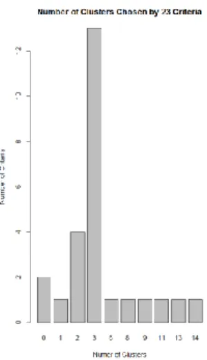
Thus, we decided to use at a second stage the NbClust package in R which provides 30 indices for determining the number of clusters (Charrad et al., 2014). In this instance, 23 indices were used to determine the optimum number of clusters, which was found to be 3. Among the 23 indices, 13 of them proposed 3 as the best number of clusters (Figure 2).
Figure 2. NbClust package determined the suggested number of clusters for the dataset
13
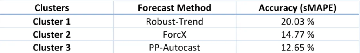
In Table 6 (Appendix A) we see that the RBF forecasting method (Appendix C) with 16.42% performs best for aggregate selection, which is followed by ForcX (16.48%) and AutoBox2 method (16.59%). When the yearly series is clustered using k-medoids technique, it is found that ROBUST-Trend (20.03%) worked best for cluster 1, followed by AutBox2 (21.02%). For cluster 2, ForcX (14.77%) and ROBUST-Trend (14.97%) performed best. For cluster 3, PP-Autocast (12.65%) performed best, followed by Dampen (12.66%) and Comb S-H-D (13.06%). So, there is not any forecasting method that works best for all clusters (Table 1).
Clusters Forecast Method Accuracy (sMAPE) Cluster 1 Robust-Trend 20.03 %
Cluster 2 ForcX 14.77 %
Cluster 3 PP-Autocast 12.65 %
Table 1. Best performing forecast method for each cluster with accuracy for 645 yearly series (k-medoids)
The number of observations in cluster 1, cluster 2 and cluster 3 are 180, 276 and 189 respectively (Table 11, Appendix A). So, when the weighted average of accuracy measure (best performing forecasting method for each cluster) for these 3 clusters is taken (Table 1), the overall performance for the yearly M3-dataset for sMAPE is 15.61%; which is lower than the best method without clustering i.e. RBF which has error of 16.42%. So, clustering the yearly series first and then forecasting produced a better result. Table 11 indicates that almost all the data of MACRO type are in cluster 2 and more than half of the data of type INDUSTRY are in cluster 1.
5.2 Random forests: 2 clusters
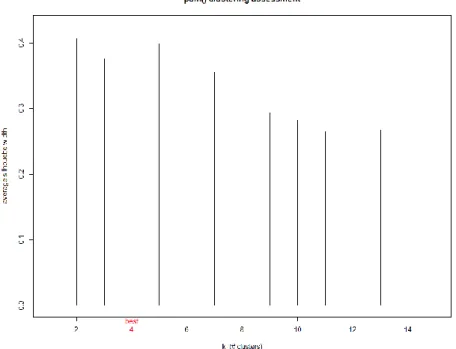
Partitioning Around Medoids (PAM) is a simple gradient descent procedure to directly minimize the within-group dissimilarity. In this, clustering is represented by medoids: given a set of medoids, each point is assigned to the closest medoid cluster. PAM clustering is very reliable and robust but is very slow when compared with other clustering techniques such as k-means (Kaufman, and Rousseeuw, 2009). Clustering through random forests is performed by using PAM. Firstly, the optimum number of clusters for the random forests clustering is found by calculating the average silhouette width for clusters ranging from 2 to 15. It is found that 4 is the optimum number of clusters for our dataset (Figure 3). The average silhouette width for k=2 clusters is also close to the value of k=4 clusters. Then, by using an alternative partitioning around medoid function called "pamNew", a variant of PAM, clusters are obtained. “pamNew” corrects the clustering membership assignment by taking account of the silhouette strength which is standard output of PAM (Shi et al., 2004).
14
Figure 3. PAM Plot to find optimum number of clusters for Random Forests
When we use 2 clusters, Robust-Trend (16.81%) worked best for cluster 1, followed by AutoBox2 (17.62%). For cluster 2, ForcX (14.77%) performed the best. There are other methods such as RBF (15.15%) and PP-Autocast (15.56%) which also performed better and are close enough (Table 7, Appendix A). So, here too, there is no one particular forecast method that works perfect for both the clusters. Robust -Trend method performs the best for Cluster 1 and ForcX method works well for Cluster 2 (Table 2).
Clusters Forecast Method Accuracy (sMAPE) Cluster 1 Robust-Trend 16.81 %
Cluster 2 ForcX 14.77 %
Table 2. Best performing forecast method for each cluster with accuracy for 645 yearly series (random forests for 2 clusters)
The number of observations in cluster 1 and cluster 2 are 273 and 372 respectively (Table 12, Appendix A). This clustering approach resulted in an overall sMAPE of 15.63% for the entire dataset, better than aggregate selection result but still marginally worse than k-medoids with three clusters. Table 12 shows that most of the Demographic time series are in cluster 2 which indicates that these type of data are homogenous.
15
5.3 Random forests: 4 clusters
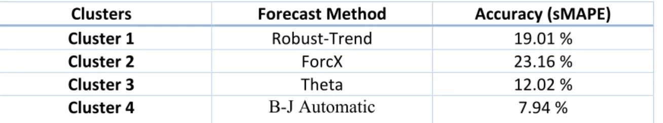
When we use random forests with 4 clusters, Robust -Trend (19.01%) worked best for cluster 1, followed by Theta (19.95%). For cluster 2, ForcX (23.16%) performed the best. For cluster 3, Theta (12.02%), Comb S-H-D (12.07%) and RBF (12.09%) performed the best. For cluster 4, B-J Automatic (7.94%) performed the best, followed by Robust-Trend (8.15%) and ForecastPro (8.48%).
Clusters Forecast Method Accuracy (sMAPE) Cluster 1 Robust-Trend 19.01 %
Cluster 2 ForcX 23.16 %
Cluster 3 Theta 12.02 %
Cluster 4 B-J Automatic 7.94 %
Table 3. Best performing forecast method for each cluster with accuracy for 645 yearly series (random forests for 4 clusters)
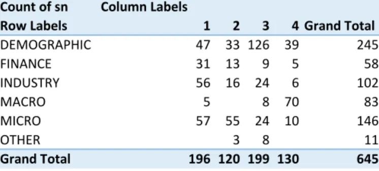
The number of observations in cluster 1, cluster 2, cluster 3 and cluster 4 are 196, 120, 199 and 131 respectively (Table 13, Appendix A), giving us overall a sMAPE of 15.40% which is lower than the best method without clustering and is the best performing approach so far. Table 13 shows that most of the data of type Macro is in cluster 4 and more than half of the data of type Demographic is in cluster 3. The Macro data are quite homogenous, for which Robust-Trend method seems to be working well.
5.4
k
-NN clustering: 3 clusters
The ‘specClust’ package in R was used to determine the optimum number of clusters for clustering using k-NN. The ratio of ‘between cluster sum of squares’ (between_SS) to ‘total sum of squares’ (total_SS= between_SS + totalwithin_SS) should be maximum in order to select particular number of clusters and it is found that the ratio is maximum (85.7%) when there are 4 clusters, compared to 3 clusters (80.8%) and 5 clusters (82.5%). Thus, we selected 4 clusters for k-NN clustering of the 645 yearly series. Nevertheless, in order to empirically check and validate the result, analysis is done by taking 3 and also 4 clusters.
16
For cluster 1, ForcX (14.77%) and Robust-Trend (14.97%) were the top performers. Robust-Trend worked best for cluster 2 (20.03%), followed by AutBox2 (21.02%). For cluster 3, PP-Autocast (12.65%) performed the best, followed by Dampen (12.66%) and Comb S-H-D (13.06%).
Clusters Forecast Method Accuracy (sMAPE)
Cluster 1 ForcX 14.60 %
Cluster 2 Robust-Trend 20.37 %
Cluster 3 Robust-Trend 15.08 %
Table 4. Best performing forecast method for each cluster with accuracy for 645 yearly series (k-NN for 3 clusters)
The number of observations in cluster 1, cluster 2 and cluster 3 are 245, 105 and 295respectively (Table 14, Appendix A) and the overall sMAPE is 15.75%. Table 14 shows that most of the Demographic data are in cluster 1 while the Macro data in cluster 3. Robust-Trend works well for the cluster with the Macro data.
5.5
k
-NN clustering: 4 clusters
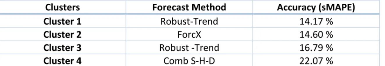
When employing four clusters, Robust-Trend (14.17%) worked best for cluster 1, followed by ForcX (14.41%) and AutBox2 (14.49%). For cluster 2, ForcX (14.60%) worked best, followed by Single (14.72%) and RBF (14.75%). For cluster 3, Robust-Trend (16.79%) performed the best, followed by AutoBox2 (18.19%) and ForcX (18.49%). For cluster 4, Comb S-H-D (22.07%) performed the best, followed closely by Theta (22.15%), PP-Autocast (22.24%) and Dampen (22.33%) (Table 10, Appendix A).
Clusters Forecast Method Accuracy (sMAPE) Cluster 1 Robust-Trend 14.17 %
Cluster 2 ForcX 14.60 %
Cluster 3 Robust -Trend 16.79 %
Cluster 4 Comb S-H-D 22.07 %
Table 5. Best performing forecast method for each cluster with accuracy for 645 yearly series (k-NN for 4 clusters)
The number of observations in cluster 1, cluster 2, cluster 3 and cluster 4 are 235, 236, 96 and 79 respectively (Table 15, Appendix A) and the overall sMAPE is 15.70% which is slightly lower than the 3 cluster version of k-NN.
17
6. Implications for theory and practice
Since this study provides preliminary evidence that cluster selection seems to be a viable alternative to aggregate selection, we can claim we corroborated with empirical evidence on the stream of theory arguing for first filtering, clustering and mining the data before you apply any extrapolative technique. This is the main theoretical and methodological contribution of our research.
For practitioners there are far more takeaways. This is something that can be done and implemented in practice quite easily. So practitioners should neither follow a ‘one size fits all’ approach, where one extrapolation method is used from your entire data; nor try use a different method for each series, as overfitting a method to the data will provide less accurate out-of-sample forecasts as literature suggests. The golden-rule solution might be somewhere in the middle, where first clustering, and then forecasting might outperform both former approaches.
The latter is also an important recommendation for software designers per s , and most specifically Forecasting Support Systems designers, where features for clustering before applying extrapolation techniques, should be offered to users as an alternative to expert systems that aim to individual series/model selection only.
7. Conclusion and Future Research
When the 645 yearly series dataset is first clustered, the accuracy of the forecasts seems to be improved, thus cluster selection is a promising alternative to both aggregate selection – that has been promoted from forecasting competitions (Makridakis and Hibon, 2000), as well as individual selection that is promoted form forecasting support systems vendors like Forecastpro. Among the three clustering methods applied, the random forests clustering method worked better than the other two techniques, i.e. k-medoids and k-NN.
18
Random forests is empirically proven in this study to be the best clustering method for cluster selection forecasting in between the three clustering approaches, both overall (for any number of identifired clusters) as well as for the maximum number of clusters i.e. four clusters in this study: the latter is very important as it could be claimed that the comparison is fair in between the clustering methods only when the number of clusters is fixed4; although obviously each method
might determine different clusters.
As in any other research that is based in one dataset, despite that being non-homogeneous and thus results can be generalised, the fact that one frequency (annual data) is used is a limitation of this study. This has been imposed for a very good reason, as seasonality would add another layer of complexity in the clustering algorithms’ ability to classify effectively the series. In any case, this is something that can be done as further research, and we leave that for the future where similar analysis can be performed on the quarterly and monthly data of the M3 or even M45.
To that end, there is also a lot of scope for more studies towards that direction, as given big data predictive analytics will be prevailing the analysis of data in the years to come, individual selection of forecasting algorithms might prove to be a very expensive exercise (computationally and literally monetary…), and as such effective (first) clustering and (then) forecasting could save a lot of time and money; and potentially even improve forecasting accuracy as the preliminary empirical evidence of this study suggests.
4 Given that in this study we chose the forecasting methods ex-post. Nevertheless as this is a clustering empirical evaluation rather than a forecasting one it is preferred all three approaches – individual selection, cluster selection and aggregate selection – to use the same extrapolations.
19
References
Anderberg, M. R. (1973). Cluster analysis for researchers. New York: Academic Press.
Agrawal, R., Faloutsos, C. and Swami, A. (1993) ‘Efficient similarity search in sequence databases’, Lecture Notes in Computer Science, pp. 69–84
Breiman, L., Friedman, J. H., Olshen, R. A. and Stone, C. J. (1984). Classification and Regression Trees, Wadsworth, Belmont, California.
Breiman, L. (1996) ‘Bagging predictors’, Machine Learning, 24(2), pp. 123–140 Breiman, L (2001). Random Forests. Machine Learning, 45:5-32
Breiman, L (2002). Using models to infer mechanisms. IMS Wald Lecture 2. [online] URL: http://oz.berkeley.edu/users/breiman/ wald2002 2.pdf. 15, 59-71
Bubeck, S. and Project,S. (2009) 'Nearest Neighbor Clustering: A Baseline Method for Consistent Clustering with Arbitrary Objective Functions', Journal of Machine Learning Research 10, pp. 657-698
Charrad, M., Ghazzali, N., Boiteau, V. and Niknafs, A. (2014) ‘An R Package for Determining the Relevant Number of Clusters in a Data Set’, Journal of Statistical Software, 61(6).
Clark, L. A. and Pregibon, D. (1992). Tree-based models, in J. M. Chambers and T. J. Hastie (eds),
Statistical Models in S, Wadsworth & Brooks/Cole, Pacific Grove, CA.
Collopy, F. and Armstrong, J. S. (1992) , “Rule-based forecasting: Development and validation of an expert systems approach to combining time series extrapolations,” Management Science, 38, 1394-1414.
Cormack, R. M. (1971) ‘A review of classification’, Journal of Royal Statistical Society, Series A(134), pp. 321–367.
Duda, R. ., Hart, P. and Stork, D. (2001) Pattern Classification. 2nd edn. Wiley.
Everitt, B. S. (1974) Cluster analysis. London: Heinemann Educational [for] the Social Science Research Council.
20
Fildes, R. and Petropoulos, F. (2015) ‘Simple versus complex selection rules for forecasting many time series’, Journal of Business Research, 68(8), pp. 1692-1701.
Gardner, E. S. (2006) ‘Exponential smoothing: The state of the art—Part II’, International Journal of Forecasting, 22(4), pp. 637–666.
Gardner, E.S., Jr., and McKenzie, E. (1985) ‘Forecasting trends in time series’, Management Science, 31, pp. 1237-1246.
Goldstein, B. A., Polley, E. C. and Briggs, F. B. S. (2011) ‘Random Forests for Genetic Association Studies’, Statistical Applications in Genetics and Molecular Biology, 10(1), pp. 1–34. Holt, C. C. (2004) ‘Forecasting seasonals and trends by exponentially weighted moving averages’,
International Journal of Forecasting, 20(1), pp. 5–10.
Hyndman, R. J. and Koehler, A. B. (2006) ‘Another look at measures of forecast accuracy’,
International Journal of Forecasting, 22(4), pp. 679–688.
Iglesias, F. and Kastner, W. (2013) ‘Analysis of Similarity Measures in Times Series Clustering for the Discovery of Building Energy Patterns’, Energies, 6(2), pp. 579–597.
Iverson, L. R. and Prasad, A. M. (1998) ‘Predicting Abundance of 80 Tree Species Following Climate Change in the Eastern United States’, Ecological Monographs, 68(4).
James, William. 1977. “The One and the Many,” The Writings of William James. Ed. John J. McDermott. Chicago: The University of Chicago Press.
Jenkins, G. M. and Box, G. E. P. (1976) Time Series Analysis: Forecasting and Control. San Francisco: Holden-Day.
Kaufman, L and Rousseeuw, P. J. (2009), Finding groups in data: an introduction to cluster analysis. John Wiley & Sons, vol. 344.
Keogh, E. (2002) ‘Exact Indexing of Dynamic Time Warping’, VLDB ’02: Proceedings of the
28th International Conference on Very Large Databases, , pp. 406–417.
Lorr, M. (1983) Cluster analysis for social scientists. 1st edn. San Francisco: Jossey-Bass Inc. U.S.
21
Makridakis, S., Andersen, A., Carbone, R., Fildes, R., Hibon, M., Lewandowski, R., Newton, J., Parzen, E. and Winkler, R. (1982) ‘The accuracy of extrapolation (time series) methods: Results of a forecasting competition’, Journal of Forecasting, 1(2), pp. 111–153
Makridakis, S., Wheelwright, S.C. & Hyndman, R.J. (1998) Forecasting Methods and Applications, 3rd edition, New York: Wiley.
Makridakis, S., Chatfield, C., Hibon, M., Lawrence, M., Mills, T., Ord, K. and Simmons, L. F. (1993) ‘The M2-competition: A real-time judgmentally based forecasting study’, International Journal of Forecasting, 9(1), pp. 5–22.
Makridakis, S. and Hibon, M. (2000) ‘The M3-Competition: results, conclusions and implications’, International Journal of Forecasting, 16(4), pp. 451–476.
Makridakis, S., Spiliotis, E. and Assimakopoulos, V. (2019) ‘The M4 Competition: 100,000 Time Series and 61 Forecasting Methods", International Journal of Forecasting, forthcoming
Nikolopoulos, K. and Thomakos, D. D. (2019), Forecasting with the Theta Method: Theory Applications, Wiley: New Jersey.
Nikolopoulos, K., Goodwin, P., Patelis, A. and Assimakopoulos, V. (2007), "Forecasting with cue information: a comparison of multiple regression with alternative forecasting approaches".
European Journal of Operational Research 180(1): 354-368.
Moore, D. M., Lees, B. G. and Davey, S. M. (1991) ‘A new method for predicting vegetation distributions using decision tree analysis in a geographic information system’, Environmental Management, 15(1), pp. 59–71
Petropoulos, F., Makridakis,S.,Assimakopoulos,V.,Nikolopoulos,K. (2014). ‘'Horses for Courses' in demand forecasting’, European Journal of Operational Research, 237(1), pp. 152–163
Prasad, A. M., Iverson, L. R. and Liaw, A. (2006) ‘Newer Classification and Regression Tree Techniques: Bagging and Random Forests for Ecological Prediction’, Ecosystems, 9(2), pp. 181– 199.
Rafiei, D. and Mendelzon, A. (1997) ‘Similarity-based queries for time series data’, Proceedings of the 1997 ACM SIGMOD international conference on Management of data - SIGMOD ’97.
22
Reilly, D. (2000) ‘The AUTOBOX system’, International Journal of Forecasting, 16(4), pp. 531– 533.
Ripley, B. D. (1996) Pattern recognition and neural networks. 1st edn. Cambridge: Cambridge University Press.
Shi, T., Seligson, D., Belldegrun, A. S., Palotie, A. and Horvath, S. (2004) ‘Tumor classification by tissue microarray profiling: random forest clustering applied to renal cell carcinoma’, Modern Pathology, 18(4), pp. 547–557.
Taylor, J. W. (2003) ‘Exponential smoothing with a damped multiplicative trend’, International Journal of Forecasting, 19(4), pp. 715–725.
Teraoka, R. (2014) ‘Grouping time series via random forests for more effective forecasting extrapolation.’, The University of Manchester Library, MSc Dissertation Thesis, MSc Business Analytics: Operational Research and Risk Analysis
Wu, X., Wu, Z. and Li, K. (2008) ‘Classification and Identification of Differential Gene Expression for Microarray Data: Improvement of the Random Forest Method’, 2008 2nd International Conference on Bioinformatics and Biomedical Engineering, pp. 763–766.
23
Appendix A: Additional Tables
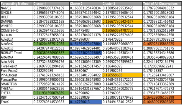
Table 6. Accuracy measure (sMAPE) for different clusters and forecasting methods for 645 yearly series (k-medoids)
Table7. Accuracy measure (sMAPE) for different clusters and forecasting methods for 645 yearly series (random forests for 2 clusters)
Forecasting Method Cluster 1 Cluster 2 Cluster 3 Total of All Observations
NAIVE2 0.239009607374159 0.166883125476834 0.138856199535496 0.178798904916532 SINGLE 0.239656573748046 0.165657413624042 0.137883759686406 0.178170015528083 HOLT 0.229939898106062 0.198793049952668 0.173951936932544 0.200206169808184 DAMPEN 0.218475258321628 0.176460639252693 0.126677806424577 0.173598121466483 WINTER 0.229939898106062 0.198793049952668 0.173951936932544 0.200206169808184 COMB S-H-D 0.216209475116836 0.168475483 0.130660584787705 0.170715952512349 B-J auto 0.233778437658904 0.163217040721378 0.143952276574698 0.177263569442358 AutoBox1 0.272907023972458 0.204296037 0.178470865 0.215875913089812 AutoBox2 0.210204567512035 0.151391273497884 0.144988539668902 0.165928135868225 AutoBox3 0.242072478122633 0.189874629694401 0.204648681102422 0.208770611761375 ROBUST-Trend 0.200389820903857 0.149723023075805 0.198441476303443 0.178138234345686 ARARMA 0.242245487899599 0.169265215083497 0.148535932009451 0.183557640829083 Auto-ANN 0.227324388296736 0.190713009443389 0.269927997599823 0.224141972164579 Flors-Pearc1 0.216977002984198 0.167132425817457 0.136446895 0.17205096612241 Flors-Pearc2 0.232292989 0.16830467 0.141902264 0.178425357 PP-Autocast 0.217410713248162 0.171824817094822 0.126558686 0.171282433419607 ForecastPro 0.219980429000765 0.159605158245953 0.146843559172205 0.172714625704756 SMARTFCS 0.227208263614129 0.166581267263089 0.144876520124786 0.177140433362389 THETAsm 0.230801416628236 0.168164331827667 0.146231680025779 0.179217671476573 THETA 0.211931390076339 0.162390082 0.17296996 0.179315713486237 RBF 0.212471007503494 0.155539839 0.131007312779495 0.164239006108298 ForcX 0.222769614539333 0.147750613 0.134491554012526 0.164800935805285
Forecasting Method Cluster 1 Cluster 2 Total of All Observations
NAIVE2 0.206450204161123 0.158506419180583 0.178798904916532 SINGLE 0.205917802985679 0.157806719893881 0.178170015528083 HOLT 0.198768450674233 0.201261270140357 0.200206169808184 DAMPEN 0.192267015091694 0.159897562435077 0.173598121466483 WINTER 0.198768450674233 0.201261270140357 0.200206169808184 COMB S-H-D 0.185480424118529 0.159880735446522 0.170715952512349 B-J auto 0.197125546488441 0.162687441126283 0.177263569442358 AutoBox1 0.224308615297181 0.20968739776021 0.215875913089812 AutoBox2 0.176208158830791 0.158383925468278 0.165928135868225 AutoBox3 0.210791033966841 0.207287882562203 0.208770611761375 ROBUST-Trend 0.168175535835245 0.185449569542863 0.178138234345686 ARARMA 0.200617479195951 0.171037920737271 0.183557640829083 Auto-ANN 0.219180000914024 0.227783418808133 0.224141972164579 Flors-Pearc1 0.183948092893362 0.163320010185665 0.17205096612241 Flors-Pearc2 0.201207413195906 0.161706266710208 0.178425356618106 PP-Autocast 0.191458621521134 0.156475714732201 0.171282433419607 ForecastPro 0.187688088035232 0.161726036413842 0.172714625704756 SMARTFCS 0.192161288290715 0.166117064019828 0.177140433362389 THETAsm 0.196865947218728 0.166266114278704 0.179217671476573 THETA 0.183624945094734 0.176153293515485 0.179315713486237 RBF 0.181517979598412 0.151558469111524 0.164239006108298 ForcX 0.188007462168255 0.147770339845364 0.164800935805285
24
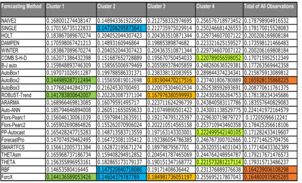
Table 8. Accuracy measure (sMAPE) for different clusters and forecasting methods for 645 yearly series (random forests for 4 clusters)
Table 9. Accuracy measure (sMAPE) for different clusters and forecasting methods for 645 yearly series (k-NN for 3 clusters)
Forecasting Method Cluster 1 Cluster 2 Cluster 3 Cluster 4 Total of All Observations
NAIVE2 0.230634635132952 0.238474578306359 0.12567242100258 0.125917129838381 0.178798904916532 SINGLE 0.229911529819213 0.238402230747521 0.124547790667377 0.125677268233113 0.178170015528083 HOLT 0.208388748561916 0.363964828146483 0.150130293607121 0.112496771013347 0.200206169808184 DAMPEN 0.204864972472547 0.278125701404729 0.123567401465456 0.105742417412739 0.173598121466483 WINTER 0.208388748561916 0.363964828146483 0.150130293607121 0.112496771013347 0.200206169808184 COMB S-H-D 0.202261675730564 0.275003543537093 0.120788305534319 0.102528266423615 0.170715952512349 B-J auto 0.221656142486258 0.265473326053389 0.131627058362043 0.098013852080626 0.177263569442358 AutoBox1 0.249751993637518 0.352550257260074 0.163592637612591 0.117767995678325 0.215875913089812 AutoBox2 0.203145337394403 0.24453562833323 0.132319121591097 0.088025808466303 0.165928135868225 AutoBox3 0.231373176318601 0.332221862209658 0.179530347834673 0.104692666743375 0.208770611761375 ROBUST-Trend 0.190194511096845 0.333986240755282 0.134970552145562 8.15538031327069E-02 0.178138234345686 ARARMA 0.224077332537644 0.312836264497629 0.133315620043982 7.94302368619344E-02 0.183557640829083 Auto-ANN 0.224066459541411 0.257326356250266 0.25170267151063 0.150279019812141 0.224141972164579 Flors-Pearc1 0.204961513984938 0.278653039923797 0.128859607916578 8.94579361958198E-02 0.17205096612241 Flors-Pearc2 0.221161309213165 0.259922593124247 0.126376976050627 0.117534419877216 0.178425356618106 PP-Autocast 0.20371128052778 0.268148367971163 0.123285610907104 0.105634487367554 0.171282433419607 ForecastPro 0.211038778407913 0.268980705176023 0.133894765210309 8.48441993407832E-02 0.172714625704756 SMARTFCS 0.216801265287403 0.282096913667339 0.127236995481913 0.096112517415484 0.177140433362389 THETAsm 0.218963425535471 0.263244588711823 0.128369356398423 0.118654306326208 0.179217671476573 THETA 0.19957902834967 0.331690756531001 0.120207000220708 9.78401665224985E-02 0.179315713486237 RBF 0.203384056431757 0.250821112293313 0.120936302693445 0.0908856959392 0.164239006108298 ForcX 0.212971004081284 0.231640475621948 0.122167136483589 9.50089279359466E-02 0.164800935805285
Forecasting Method Cluster 1 Cluster 2 Cluster 3 Total of All Observations
NAIVE2 0.149529999954773 0.242032565157251 0.18060008251096 0.178798904916532 SINGLE 0.147856744495399 0.240931381784715 0.18100665263338 0.178170015528083 HOLT 0.202450476732422 0.210352811383322 0.194730737395206 0.200206169808184 DAMPEN 0.149085532758613 0.206616741955767 0.182203643778528 0.173598121466483 WINTER 0.202450476732422 0.210352811383322 0.194730737395206 0.200206169808184 COMB S-H-D 0.151662490261543 0.205409287415359 0.17419153924669 0.170715952512349 B-J auto 0.158696432199455 0.229538098784933 0.174077545861141 0.177263569442358 AutoBox1 0.19735805927214 0.264869214322758 0.21381685395717 0.215875913089812 AutoBox2 0.156185951267123 0.224468385209504 0.153182742805293 0.165928135868225 AutoBox3 0.213137852871965 0.241759794372535 0.193401668553693 0.208770611761375 ROBUST-Trend 0.200053812611685 0.203712400736524 0.150834491477183 0.178138234345686 ARARMA 0.159434494498436 0.22377365895411 0.189277942347325 0.183557640829083 Auto-ANN 0.257316532585378 0.233733471183493 0.193176295215152 0.224141972164579 Flors-Pearc1 0.159440442369257 0.210658695945092 0.168782378624585 0.17205096612241 Flors-Pearc2 0.155791458473618 0.243584877751469 0.174030628910978 0.178425356618106 PP-Autocast 0.148834867104885 0.20498203878705 0.177930552685798 0.171282433419607 ForecastPro 0.164076749509587 0.222787984302017 0.162065734230534 0.172714625704756 SMARTFCS 0.16319230856805 0.239971234054493 0.166360963877446 0.177140433362389 THETAsm 0.159484793880671 0.229457184555207 0.177724132960437 0.179217671476573 THETA 0.181655368251751 0.20786001619431 0.167212773818785 0.179315713486237 RBF 0.147355637389356 0.212060303890789 0.161239647020094 0.164239006108298 ForcX 0.14607449548897 0.238424120122196 0.154148540972137 0.164800935805285
25
Table 10. Accuracy measure (sMAPE) for different clusters and forecasting methods for 645 yearly series (k-NN for 4 clusters)
Table 11. Type of series and cluster numbers for yearly data (k-medoids)
Table 12. Type of series and cluster numbers for yearly data (random forests for 2 clusters)
Forecasting Method Cluster 1 Cluster 2 Cluster 3 Cluster 4 Total of All Observations
NAIVE2 0.168001274438147 0.148943361922566 0.212758332974695 0.256576718973452 0.178798904916532 SINGLE 0.170156735122833 0.147206295873641 0.212735975029914 0.250246681426553 0.178170015528083 HOLT 0.183867089670274 0.204052044307423 0.204363510871344 0.229734607007122 0.200206169808184 DAMPEN 0.170598067421213 0.14893160946864 0.19885389874682 0.223321625159527 0.173598121466483 WINTER 0.183867089670274 0.204052044307423 0.204363510871344 0.229734607007122 0.200206169808184 COMB S-H-D 0.162071386432398 0.151687652728889 0.195670750454033 0.220789056598052 0.170715952512349 B-J auto 0.159848893746309 0.158565006979469 0.205589378405859 0.248260636529381 0.177263569442358 AutoBox1 0.197071026911287 0.199788586331371 0.238338132083955 0.289844374234341 0.215875913089812 AutoBox2 0.144989287112494 0.155650819012698 0.181904470217516 0.237401806780889 0.165928135868225 AutoBox3 0.177682442843737 0.21624530700493 0.220075304602534 0.262538592693691 0.208770611761375 ROBUST-Trend 0.141783800642007 0.202263087371104 0.167976380599993 0.224305656264753 0.178138234345686 ARARMA 0.168966469813085 0.16079591495717 0.223711624296739 0.243840583117786 0.183557640829083 Auto-ANN 0.185794646894008 0.260511655059633 0.210749890501422 0.243001138529775 0.224141972164579 Flors-Pearc1 0.156046130061039 0.159798412635911 0.192174795125397 0.229630719879727 0.17205096612241 Flors-Pearc2 0.165902690864826 0.155262070906024 0.202210514565158 0.253710943460358 0.178425356618106 PP-Autocast 0.165428247715283 0.148713583713559 0.197163143303001 0.222499542140105 0.171282433419607 ForecastPro 0.147074929462495 0.164723081105412 0.192386054786385 0.246767300702666 0.172714625704756 SMARTFCS 0.156612005731384 0.162872195671274 0.18979879567701 0.263205514031043 0.177140433362389 THETAsm 0.165968737186734 0.159408294912852 0.204541787465069 0.244764248954787 0.179217671476573 THETA 0.156355896953161 0.182865173179137 0.190151347168772 0.221573281217114 0.179315713486237 RBF 0.14653580416445 0.147520840718086 0.19171408636442 0.231376889376638 0.164239006108298 ForcX 0.144136589053426 0.14604379787789 0.184981736051197 0.255695217807043 0.164800935805285
Count of sn Column Labels
Row Labels 1 2 3 Grand Total
DEMOGRAPHIC 35 87 123 245 FINANCE 33 15 10 58 INDUSTRY 58 19 25 102 MACRO 2 80 1 83 MICRO 52 72 22 146 OTHER 3 8 11 Grand Total 180 276 189 645
Count of sn Column Labels
Row Labels 1 2 Grand Total
DEMOGRAPHIC 69 176 245 FINANCE 37 21 58 INDUSTRY 60 42 102 MACRO 35 48 83 MICRO 72 74 146 OTHER 11 11 Grand Total 273 372 645
26
Table 13. Type of series and cluster numbers for yearly data (random forests for 4 clusters)
Table14. Type of series and cluster numbers for yearly data (k-NN for 3 clusters)
Table 15. Type of series and cluster numbers for yearly data (k-NN for 4 clusters)
Count of sn Column Labels
Row Labels 1 2 3 4 Grand Total
DEMOGRAPHIC 47 33 126 39 245 FINANCE 31 13 9 5 58 INDUSTRY 56 16 24 6 102 MACRO 5 8 70 83 MICRO 57 55 24 10 146 OTHER 3 8 11 Grand Total 196 120 199 130 645
Count of sn Column Labels
Row Labels 1 2 3 Grand Total
DEMOGRAPHIC 142 14 89 245 FINANCE 14 23 21 58 INDUSTRY 31 46 25 102 MACRO 12 71 83 MICRO 36 22 88 146 OTHER 10 1 11 Grand Total 245 105 295 645
Count of sn Column Labels
Row Labels 1 2 3 4 Grand Total
DEMOGRAPHIC 71 139 26 9 245 FINANCE 12 14 13 19 58 INDUSTRY 16 30 19 37 102 MACRO 74 8 1 83 MICRO 62 35 37 12 146 OTHER 10 1 11 Grand Total 235 236 96 78 645
27
Appendix B: Distance Measures
Euclidean distance, root mean square distance, and Mikowski distance
If Pi and Qi are d-dimensional vectors, the Euclidean distance is defined as:
𝑑𝐸𝑈𝐶 = √∑(𝑃𝑖 − 𝑄𝑖)2
𝑑
𝑘=1
The root mean square distance (or average geometric distance) is defined as:
𝑑𝑅𝑀𝑆= 𝑑𝐸𝑈𝐶/𝑛
Mikowski distance is a generalization of Euclidean distance, which is defined as:
𝑑𝑀𝐾 = √∑(𝑃𝑖− 𝑄𝑖)𝑝
𝑑
𝑘=1
𝑝
Pearson’s correlation coefficient and related distances
If xi and vj each be a P-dimensional vector and Pearson’s correlation factor between xi and vj, Cc,
is defined as: Cc = ∑ (𝑥𝑖𝑘− 𝑢𝑥𝑖𝑘)(𝑣𝑗𝑘− 𝑢𝑣𝑗𝑘) 𝑃 𝑘=1 𝑆𝑥𝑖𝑆𝑦𝑗 where 𝑢𝑥𝑖𝑘 =𝑃1∑𝑃𝑘=1𝑥𝑖𝑘,𝑆𝑥𝑖 = [∑𝑃𝑘=1(𝑥𝑖𝑘− 𝑢𝑥𝑖𝑘)]0.5
Dynamic time warping distance
A distance measure specially addressed to time series comparison is the Dynamic Time Warping (DTW) distance (Keogh, 2002). This is a technique which is being used in variety of applications such as speech recognition and time series similarity search for performing time alignment. This measure allows a non-linear mapping of two vectors by minimizing the distance between them. It can be used for vectors of different lengths: Q=q1, q2, . . . , qi, . . . , qn and R =r1, r2, . . . , rj , . . . ,
28
The metric establishes an n-by-m cost matrix C which contains the distances (usually Euclidean) between two points qi and rj. A warping path, W =w1, w2, …. wk, . . . , wK where max(m, n) ≤
K ≤ m + n − 1, is a set of matrix elements that satisfies three constraints: continuity, boundary
condition and monotonicity (Iglesias and Kastner, 2013). There are many paths that accomplish the introduced conditions; the one that minimizes the warping cost is the DTW distance. Mathematically, it is represented as:
d𝐷𝑇𝑊 = 𝑚𝑖𝑛
∑𝐾 𝑤𝑘
𝑘=1
𝐾
Short time series distance
Short time series distance is the sum of the squared differences of the slopes in two time series that are being compared. Mathematically, the distance between two time series xi and vj is defined as:
𝑑𝑆𝑇𝑆 = √∑ (𝑣𝑗(𝑘+1)− 𝑣𝑗𝑘 𝑡(𝑘+1)− 𝑡𝑘 − 𝑥𝑖(𝑘+1)− 𝑥𝑖𝑘 𝑡(𝑘+1)− 𝑡𝑘 ) 2 𝑃 𝑘=1
29
Appendix C: Forecasting methods used in the M3-competion
(Makridakis and Hibon, 2000)
Naïve2
The fundamental philosophy of Naïve is that it assumes no existence of trend and taking the last known observation as the prediction for all forecasting horizons. Naïve 2 is applying seasonal adjustment over the forecasts of Naïve.
Single
Single Exponential Smoothing (SES) is the basic model of exponential smoothing dated back to the work of Bob Brown in the middle of the previous century, and its most important feature is the exponentially decreasing weight over the past obdservations. This method is suitable for forecasting time series data with no trend or seasonal pattern and is equivalent to an ARIMA(0,1,1) (Makridakis et al, 1998).
Holt
Holt (republished in 2004) is designed to capture explicit trend within the Exponential Smoothing Family. It is an extended version of single exponential smoothing to allow forecasting of data with a trend.The forecasts provided by Holt display a constant trend (increasing or decreasing) indefinitely into the future.This method is equivalent to ARIMA(0,2,2)
Dampen
This method is similar to Holt but with a parameter that “dampens” the trend to a flat line in the future. It is very successful method and is one of most popular individual methods in industry and academia when forecasts are required automatically for many series (Gardner and McKenzie, 1985). If the time series is indeed showing a strong trend, it is similar to forecasts of Holt and if there is no trend, it will produce similar forecasts to that of SES.
Winter
Winter’s method is the extended version of Holt’s method for seasonal data.There are two variations to this method that differ in the nature of the seasonal component: the additive method and multiplicative method. The former is preferred when the seasonal variations are constant
30
through the series, while the latter is preferred when the seasonal variations are changing proportional to the level of the series.
Comb S-H-D
This method is an equal-weighted combination of Single, Holt and Dampen methods. It ofen performs better than all three of its components.
Robust Trend
It is a non-parametric linear model with median based trend estimate, which is different than Holt (Makridakis and Hibbon, 2000). This method is not influenced by extreme outliers since the parameter for identifying trend is measured by the median of the differenced series.
B-J Automatic
This method is an automatic version of ARIMA (Jenkins and Box, 1976) and it may be considered as a text-book approach to Time-Series forecasting (Makridakis et al, 1998.
Autobox1-2
The Autobox1 is pure ARIMA and contains no outlier detection and produces similar forecasts to that of B-J Auto (Reilly, 2000). The Autobox2 has residual analysis included along with the original ARIMA process. The different types of residuals from 4 types of possible auxiliary variables, i.e., pulse, seasonal pulse, Level Shift and Local Time Trends are examined.
PP-Autocast
This method is from the exponential smoothing family and is just an automatic dampen trend and is similar to Dampen method.
ForecastPRO
ForecastPro is a commercial software (www.forecastpro.com) that employs a selection protocol among popular forecasting techniques, mainly exponential smoothing based. The exact details of the algorithm have not been made publicly available but the success of the software is longitudinal claiming the second-best position in the M3 competition and outperforming the Theta method in the M4 competition.
31
Automat ANN
Artificial Neural Networks are universal function approximators and are capable of exploiting non-linear relationships. This particular M3 model attempts to develop an automatic procedure for selecting the architecture of an artificial neural network for the purpose of forecasting.
THETA-sm
This method works well for time series data that are characterized by changing patterns. The process of fitting the data depends on this very feature of identification of noisy or changing patterns in the time series.
Smart FCs
This method automatically conducts a mini competition among the methods of simple moving average, linear moving average, single exponential smoothing, double exponential smoothing, Winters’ additive and Winters’ multiplicative exponential smoothing. This method computes the out-of-sample forecast errors by using historical data.
RBF (Rule-based Forecasting)
The RBF method used in M3-competition is slightly different from the original method developed by Armstrong and Collopy (1992). Some additional modifications were done to the original rule-based forecasting method in order to deal with different types of data. RBF is successful for a series when the following conditions are met: a) Series where the certainty is moderate to low, and b) Series where there are very low instabilities such as outliers, step changes. It proved very succesfull for yealy data and for very long forecasting horizons.
Flores-Pearce
This method, via using an expert system automatically chooses from among the following four forecasting methods: SES, SES with seasonality, Dampen and with seasonality, based on the data characteristics such as whether the data has trend or seasonality. Any outliers present in the data were removed before choosing the model. Two types of this forecast method were implemented in M3-competition data, one generated by the system and the other a slightly modified version of the expert system.
32
Appendix D: Accuracy metrics
Scale-Dependent Errors
The one-step-ahead forecast error given by et =yt −yˆt. where yt the actual and yˆt the forecast. The
two most commonly used scale-dependent measures are:
Mean absolute error (MAE) = mean (|et|),
Mean squared error (MSE) = mean (et2).
MAE is used to compare forecast methods on a single series as it is easy to compute and understand. However, it cannot be used to make comparisons between series as it makes no sense to compare accuracy on different scales.
Percentage Errors
The percentage error is given by pt = 100et/yt. These errors are scale-independent, and therefore are frequently used to compare forecast performance between different data sets. The most commonly used measure is:
Mean absolute percentage error (MAPE) = mean (|pt|)
But, these measures which are based on percentage errors have one disadvantage, i.e. they are infinite or undefined if yt = 0 for any t in the period of interest, and have an extremely skewed distribution when any yt is close to zero. Another issue with percentage errors is that they assume a meaningful zero. For example, a percentage error makes no sense when measuring the accuracy of temperature forecasts. Also, it was found that they put a heavier penalty on positive errors than on negative errors. This led to the use of the “symmetric” MAPE which was proposed by Makridakis (1993) and was used in the M3-competition (Makridakis and Hibon, 2000). It is defined as:
sMAPE = mean (200|yt − yˆt|/(yt + yˆt)).
However, if yt is zero, yˆt is also likely to be close to zero. Thus, the measure still involves division
by a number close to zero and the value of sMAPE can also be negative, so it is not really a measure of “absolute percentage errors” at all.
33
Scaled Errors
The MASE was proposed as a generally applicable measure of forecast accuracy (Hyndman and Koehler, 2006). It was proposed to scale the errors based on the in-sample MAE from the naive forecast method. Thus, a scaled error is defined as:
𝑞𝑡 =
𝑒𝑡 1
𝑛 − 1 ∑𝑛𝑖=2|𝑦𝑖 − 𝑦𝑖−1| which is independent of the scale of the data.
The mean absolute scaled error is simply written as: MASE = mean (|qt|).
The in-sample MAE is used in the denominator as it is always available and effectively scales the errors.
In conclusion, if all the series are on the same scale, then the MAE can be preferred because it is easy to explain. If all data are positive and greater than zero, the MAPE can be preferred for the same reason of simplicity. However, in situations where there are very different scales including data which are close to zero or negative, it is suggested that the MASE is the best measure of forecast accuracy.