arXiv:1404.2570v2 [cs.SI] 28 May 2014
Modelling View-count Dynamics in YouTube
C´edric Richier
∗, Eitan Altman
†, Rachid Elazouzi
∗, Tania Jimenez
∗, Georges Linares
∗and Yonathan Portilla
∗∗University of Avignon, 84000 Avignon, FRANCE Email: [email protected]
†INRIA, B.P 93, 06902 Sophia Antipollis Cedex, FRANCE Email: [email protected]
Abstract—The goal of this paper is to study the behaviour of view-count in YouTube. We first propose several bio-inspired models for the evolution of the view-count of YouTube videos. We show, using a large set of empirical data, that the view-count for 90% of videos in YouTube can indeed be associated to at least one of these models, with a Mean Error which does not exceed 5%. We derive automatic ways of classifying the view-count curve into one of these models and of extracting the most suitable parameters of the model. We study empirically the impact of videos’ popularity and category on the evolution of its view-count. We finally use the above classification along with the automatic parameters extraction in order to predict the evolution of videos’ view-count.
Keywords—YouTube,bio-inspired models, view-count.
I. INTRODUCTION
YouTube has been one of the most successful user-generated video sharing sites since its establishment in early 2005 and constitutes currently the largest share of Internet traffic. The rate of subscription to YouTube as well as the rate of submitted videos has been growing steadily ranking YouTube and none of its competitors has achieved a similar success [1], [2]. An important aspect of videos in YouTube is their popularity, which is defined as the number of view-counts. Understanding and predicting the popularity is useful from a twofold perspective: On one hand, more popular content generates more traffic, so understanding popularity has a direct impact on caching and replication strategy that the provider should adopt; and on the other hand, popularity has a direct economic impact. A number of researchers have analyzed the popularity characteristics of user-generated video content for understanding the processes governing their popularity dynam-ics [5], [10], [13], [18], [8], [6], with the aim of developing models for early-stage prediction of future popularity [19]. There has been also interest in understanding what important factors lead some videos to become more popular than others. But few works have studied the temporal aspects of the popularity dynamics using some metrics such as view-counts, ratings and number of comments [5], [9], [17].
In this paper we describe some of the most typical be-haviour of the view-count of videos in YouTube. This allows us to provide in-depth analysis and develop models that capture the key properties of the observed popularity dynamics. Our goal is to match observed video view-counts with one of several dynamic models. To select candidates for these models, we turned to bio-inspired dynamics as we believed that the propagation of a content in YouTube has a strong similarity with the temporal behaviour of an infectious disease, which is a classical topic in mathematic biology [3], [16]. Such models
of diseases spread have already been used in order to model the spread of viruses in computer networks [7], [12]. They have been also used in marketing for capturing the life cycle dynamics of a new product [4]. A large number of papers in marketing have shown that product sales life cycle follow an S-curve pattern in which the product sales initially grow at fast rate and it falls off as the limit of the market share is approached [14].
We propose several information diffusion models to clas-sify a dataset of more than 800000 videos randomly ex-tracted from YouTube and aged between 5 and 2500 days. In particular, we exhibit six mathematical models to which we fit videos in our dataset. We then propose automatic ways for associating each video to one of the considered models. The first criterion in selecting the model is related to the size of the population that may be potentially interested by the content. We differentiate between models in which the population potentially interested in the content is nearly constant (we call this the ”fixed target population property”) and those in which it grows in time (inspired by the branching process terminology, we call this ”immigration”). The fixed target population property occurs in some video categories in YouTube as news, sport and movies. Indeed, videos in these categories reach quickly the peak of the popularity and then within a short time the diffusion dies out and the view-count does not further increase.
The second criterion in the classification concerns the structural virality. A model is said to be viral (or to have the viral property) if contaminated nodes (these are the viewers of a video) have a significant role in the propagation of the video through sharing or embedding. It is non-viral if the propagation of the video essentially relies on broadcast of the video from the source (it is then said to have the broadcast property). In that case, a large fraction of potential target population can receive the information directly from the source.
Our contribution can be summarised in the following key points
• We propose six mathematical biology-inspired models and we show that at least 90% of videos in YouTube are associated to one of these six mathematical models with a Mean Error Rate less than 5%. We further show how to extract the model parameters for each video. • We study the robustness of these models to the
differ-ent thematic categories of the video in YouTube and to different values of the peak popularity of the video. We show that the fraction of videos withing a given model is quite robust and shows little dependence
on the different thematical categories of the video, except for Education category which has a different behaviour: For this category it seems that the word-of-mouth is the dominate mechanism through which contents are disseminated. The bio-inspired models that we selected are further shown to be robust with respect to the peak popularity of the video but the distribution among them is slightly different between those videos that have acquired less than 1000 views and the rest of the videos.
• In more than 80% of videos in YouTube, the potential population interested in the video increases over time. • Two of the six models (The modified negative expo-nential and modified Gompertz models) cover most of videos in our YouTube Dataset (more than 75%). Both models capture the case of immigration pro-cess in which the potential population or the ceiling value become dynamic. Further, the modified negative exponential characterizes the dynamic of a non-viral content and it predicts that the accumulated number of view doesn’t contribute to the propagation of the con-tent. This model corresponds to the scenario wherein the content has been broadcasted to a pool of users. On the other side, the Gompertz model captures viral videos in which a part of this dynamic is propagated through word-of-mouth.
• We finally use the above classification along with the automatic parameters extraction in order to predict the evolution of videos’ view-count. We consider two scenarios: In the first we use half of the view-count curve as a training sequence while in the second one, we take a fixed training sequence that corresponds to the first 50 days in the lifetime of the video. We then compare the predicted curve to the actual one and study the prediction capacity within a given error bound.
II. SETTING AND DATA
Since we intend to study different types of dynamic evolu-tion of the view-count in YouTube, we need to collect a huge number of videos which are available to the general public.
In this section we describe how we collected the dataset used in this study. On YouTube, a video is accompanied by a set of valuable data as title, upload time, view-count, related videos. The video web page also provides some statistics which are available if the content’s owner allows it.
YouTube provides two APIs which allow to retrieve some of those data : the YouTube Data API for collecting static data (which are available for every user) and the YouTube Analytics API for seeking video statistics such as dynamics of a content (which are only available for content’s owner). Since some data cannot be collected through the APIs, we used a tool named YOUStatAnalyzer [20] in order to collect all valuable data.
The collected data are stored in a noSQL database (Mon-goDB). The noSQL solution has been chosen to allow dynamic insertion of new features for future works. The dataset used for this study contains more than80000videos randomly extracted from YouTube and aged between 5 and 2500 days. This
dataset contains some static information for each video such as YouTube id, title of the video, name of the author, duration and list of related videos. It also provides the evolution of some metrics (shares, subscribers, watch time and views) in a daily form and in a cumulative form, from the upload day till the date of crawling.
III. POPULARITY GROWTH PATTERNS
We focus the analysis on view-count as the main popularity metric of a video. Previous analyses of YouTube showed a strong correlation between view-count and other metrics as number of comments, favourites and rating. Further, these metrics correlation becomes stronger with popularity [8]. We model the dynamic evolution of view-count some mathemat-ical models from the biology. We classify the evolution of view-count in YouTube using two criteria:
• Size of the target population: The target population
size is the maximum number of individuals that can be, potentially, interested by the content. A target population belongs to one of these two types: (i) a fixed finite target population or (ii) a potential target population that grows in time which we call the
immigration process.
• Virality: A content is viral if the population that has
seen the content participates actively in the dissem-ination of the content. The content spreads like a virus does in epidemics. Thus the probability that an individual who has not seen the content so far got it by someone who see it, increases in time. On the contrary, a non viral content is one for which former viewers scarcely alter the diffusion process.
In the following we describe the dynamic models in biology and their uses. These dynamic models have been hypothesised to describe the contagion phenomena and each model has its own set of assumptions about how users are infected by others. These models may provide some answers about the behaviour of users in YouTube even if this behaviour remains notoriously difficult to quantify.
A. Fixed target population
1) Viral content: To describe the viral content with fixed
target population, we use the logistic model or the Gompertz model. These models have been used in technology forecasting and are referred as ”S-shaped” curve. We test these models to capture the evolution of view-count of a video in YouTube since there is a strong similarity between a video posted in YouTube and a new product launched into the marketplace. In-deed, as showed in different problems in marketing, technology product is often growth slowly followed by rapid exponential growth and finally it falls off as limit of market share is approached.
Logistic model: The logistic model is a common sigmoid
function which describes the evolution of view-count of a video with fixed target population. This is a first order non-linear differential equation of the form
dS
Fig. 1. Example of non symmetric S-shaped behaviour of view-count in YouTube (viral).
whereSis the number of view-counts of a video andM is the maximum size of the (potential) population that could access the content. This is a standard equation in epidemiology for describing the evolution of the number of infected individuals under the assumption that all infected nodes have developed an immunity from infection or these infected nodes stay infected and will not be changed to uninfected state. Hence the infection rate is a function of the rate λ and the size of the infected population. For the YouTube case, this model corresponds to the scenario wherein users may watch a video one time and the probability to watch it again is negligible. A solution to equation (1) is given by
S(t) = M
1 + (MS−(0)S(0))e−λM t
This function shows that initial exponential growth is followed by a period in which growth starts to decrease as approaching the maximum size of population.
The S-shape of the sigmoid model curve is symmetric. But in the context of view-count, the convex phase and the concave phase could not always be symmetric. This is shown by the example in Figure 1. For covering these cases we consider the Gompertz model.
Gompertz model: A model which deals with the problem
of symmetry of the Logistic model is given by the following dynamic equation:
dS
dt =λSlog(
M
S ), (2)
This model is called Gompertz model, and has been also used as diffusion model of product growth. A solution of equation 2 is given by the Gompertz function :
S(t) =Mexp(−log( M
S(0)) exp(−λt)),
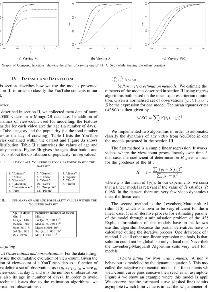
Figure 2 shows the effect of varying one ofM,λ,S(0)while keeping the others constant.
This model is similar to the logistic curve but it is not symmetric about the inflection. In general the Gompertz’s model reaches this point early in the growth trend. This
behaviour seems to fit well for some YouTube view-count evolution dynamics.
2) Non-viral content: A non viral content describes the
case where users do not contribute on the propagation of the content. This is the case when the time scale of the content diffusion is very large compared to the size of potential popu-lation. Hence this dynamic can model the case where contents gain popularity through advertisement and other marketing tools: examples are when advertisement is broadcasted to a very large pool of users of a social network and people access the content at random thereafter. Hence we assume that the evolution dynamic of the content follows the linear differential equation:
dS
dt =λ(M −S) (3)
The solution of (3) is given by :
S(t) =S(0) + (M−S(0))(1−e−λt)
B. Growing population
The assumption that the population is fixed, is often a reasonable approximation when the evolution of the popularity of a content increases quickly and dies out within a short time. But for many cases, this assumption becomes inappropriate when the time before reaching the saturation region is longer. Here we consider the case of immigration process in which the potential population growth and the dynamic of view-count of a content are intricacy linked. To capture such dependence we consider different growth scenarios that model the viral case and non viral case. In this paper we restrict our study on the case where the target population grows with a fixed speed.
1) Non-viral content : The linear growth model S(t) =
S(0) +λtdescribes in a simple way the situation where users do not contribute to propagate the content to other users but the content benefits of the immigration process which gives a linear growth of the view-count.
Another kind of non-viral curves observed are concave curves (given by the negative exponential model) which do not converge to a flat line but become linear at the horizon due to the immigration process influence. Such dynamics could be modelled by modifying solutions of equation 3 where a linear component is added:
S(t) =S(0) + (M−S(0))(1−e−λt) +kt
wherek is the rate of the target population growth. Note that
S no more respects the equation 3 but(S−kt)does.
2) Viral content : Now we consider the case when the
immigration process appears in the case of viral contents. In this dynamic the view-count curve first adopts a viral behaviour (in a S-shaped phase) and then grows linearly.
One candidate solution to describe such a behaviour of view-count is to add a linear component to the Gompertz function :
S(t) =Mexp(−log( M
S(0)) exp(−λt)) +kt
This dynamic seems to be relevant according to some examples in the dataset.
0.0 0.5 1.0 1.5 2.0
0.0
0.5
1.0
1.5
Gompertz model : varying M
t S(t) (a) Varying M 0.0 0.5 1.0 1.5 2.0 0.0 0.5 1.0 1.5
Gompertz model : varying λ
t S(t) (b) Varyingλ 0.0 0.5 1.0 1.5 2.0 0.0 0.5 1.0 1.5
Gompertz model : varying S(0)
t
S(t)
(c) VaryingS(0)
Fig. 2. Graphs of Gompertz functions, showing the effect of varying one ofM,λ,S(0)while keeping the others constant
IV. DATASET ANDDATA FITTING
This section describes how we use the models presented in section III in order to classify the YouTube contents in our dataset.
A. Dataset
As described in section II, we collected meta-data of more than 80000 videos in a MongoDB database. In addition of the dynamics of view-count used for modelling, the features we consider for each video are: the age (in number of days), the YouTube category and the popularity (i.e the total number of views at the day of crawling). Table I lists the YouTube categories contained within the dataset and Figure 3a shows their distribution. Table II summarises the values of age and popularity metrics. Figure 3b gives the ages distribution and Figure 3c is about the distribution of popularity (inlogvalues). TABLE I. LIST OF ALLYOUTUBE CATEGORIES FOUND INSIDE THE
DATASET
1. ”Animals” 7. ”Games” 13. ”Shows”
2. ”Autos” 8. ”Howto” 14. ”Sports”
3. ”Comedy” 9. ”Music” 15. ”Tech”
4. ”Education” 10. ”News” 16. ”Travel”
5. ”Entertainment” 11. ”Nonprofit”
6. ”Film” 12. ”People”
TABLE II. SUMMARY OF AGE AND POPULARITY VALUES WITHIN THE YOUTUBE DATASET
Age (in days) Popularity (number of views)
Min:5 Min:1 1st Qu.:140 1st Qu.:2,650.102 Median:393 Median:2,728.103 Mean:610,5 Mean:6,091.105 3rd Qu.:923 3rd Qu.:2,630.104 Max:2426 Max:1,746.109 B. Data fitting
a) Observations and normalisation: For the data fitting,
we only use the cumulative evolution of view-count. Given the evolution of view-count of a YouTube video as a function of time, we define a set of observations as :(yi, ti)1≤i≤nwhereyi
is the view-count at daytiandnis the number of observations
(this is also its age in number of days). In order to avoid some technical issues due to the estimation algorithms, we use normalised observations :
(yi
yn,
ti
tn)1≤i≤n
b) Parameters estimation methods: We estimate the
pa-rameters of the models described in section III using regression algorithms both based on the mean squares criterion minimisa-tion. Given a normalised set of observations(yi, ti)1≤i≤n, let S be the expression for one model. The mean squares criterion (M SC) is then given by :
M SC=X
i
(S(ti)−yi)2
We implemented two algorithms in order to automatically classify the dynamics of any video from YouTube in one of the models presented in the section III.
The first method is a simple linear regression. It works for videos where the view-count grows linearly over time t. In that case, the coefficient of determination R gives a measure for the goodness of the fit :
R= 1− P i(yi−S(ti)) 2 P i(yi−y¯)2
wherey¯is the mean of(yi)i. In our experiments, we consider
that a linear model is relevant if the value ofRsatisfies|R| ≥
0.985. In the dataset, there are very few video dynamics that meet the linear case.
The second method is the Levenberg-Marquardt Algo-rithm [15] which is known to be very efficient for the non-linear case. It is an iterative process for estimating parameters of the model through a minimisation problem of the M SC. Explicit formulation of the models have to be known to use this algorithm because the partial derivatives have to be calculated during the iterative process. One drawback of this method, like all other non-linear regression methods, is that the solution could not be global but only a local one. Nevertheless, the Levenberg-Marquardt Algorithm suits very well for our models.
c) Data fitting for Non viral contents: A non viral
behaviour is modelled by the dynamic equation 3. This model, called the negative exponential model, fits for contents which view-count curve goes concave then reaches an asymptote. In Figure 4 we show an example where this model is applied. We observe that the estimated curve (dashed line) admits an asymptote (which limit value is in fact theM parameter of the
1 2 3 4 5 6 7 8 9 11 13 15 Categories distribution over the hole dataset
0
2000
6000
10000
14000
(a) YouTube categories distribution
Ditribution of age Age P ercent of all 0.0 0.5 1.0 1.5 2.0 0 500 1000 1500 2000 2500
(b) Age distribution (in number of days)
Popularity distribution Log of popularity P ercent of all 0 5 10 15 20 25 0 2 4 6 8 10
(c) Logarithmic distribution of popularity Fig. 3. Some features distributions from the YouTube dataset.
model). This is typically the case with fixed finite population. But at the horizon, the curve that represents data (plain line) seems to follow a line with a non zero slope. This is what we call the immigration phenomena, when the size of target population increases linearly in time. In that case, we model the dynamics by the modified negative exponential functions introduced in subsection III-B1:
S(t) =S(0) + (M−S(0))(1−e−λt) +kt
This model fits better as it is shown in Figure 4c. A mixed strategy, which consists in cutting data into two subsets and then applying linear model on one subset and negative expo-nential model on the other, will be discussed later.
d) Data fitting for Viral contents: Three models have
been considered in the case of viral contents: logistic model, Gompertz model and a modified Gompertz model (see sec-tion III-B2). The first two models are for the context of fixed finite population and the third one is introduced in the case of immigration.
Figure 5 is an example where we fit these models to one YouTube content (Figure 5a). We observe that the S-shape of the logistic model curve is symmetric due to the symmetrical property of sigmoid function (Figure 5b). However, the convex phase and the concave phase are non symmetric as we can observe in Figure 5a. Hence the Logistic model does not fit well. Then, Gompertz model and modified Gompertz model are fitted to the same YouTube content. The Gompertz model (Figure 5c) fits better than the logistic model, and the modified Gompertz model (Figure 5d) describes better the behaviour of the data at the horizon (immigration phenomena).
e) Mixing linear and non-linear models: An issue that
results from the model we use is the changes of the curve dynamics at the horizon. We observe two types of behaviour at the horizon : a flat line showing that the limit of the potential population has been reached or an oblique line highlighting the fact that the population continues to grow.
The first case is coherent with the description of dynamics (then the maximum is one of the parameters of the dynamic equation of the model). However, for the second case we need to add a linear component to the solution function, implying that the initial dynamic equations are not valid anymore. Hence, we propose to adopt a two phases approach for data fitting. Figure 6 gives an example where this method is applied for a YouTube content (Figure 6a).
Given a set of observations (yi, ti)1≤i≤n, a first phase
consists in pointing out a linear behaviour from a time t =
tk, k∈1, .., n. The idea is to findkin an iterative way in order
to have a good regression line for the subset(yi, ti)k≤i≤n. The
algorithm is the following : we first fix a thresholdǫreasonably small. We then apply a linear regression with all the points. The regression line gives the set(ˆyi)i of the estimated values.
Let y¯ be the mean of (yi)i, we consider the coefficient of
determination r1 given by:
r1= 1−
Pn
i=1(yi−yˆi)2
P
i(yi−y¯)2
• if |1 −r1| ≤ ǫ, observations could be considered
as linear (the whole view-count curve could be well described by the linear model) and the process ends. • else, the first element of(yi, ti)1≤i≤nis removed from
the set and a new linear regression is done for the subset (yi, ti)2≤i≤n. That gives a new coefficient of
determinationr2
The process is repeated until the coefficient of determination
rk satisfies |1−rk| ≤ ǫ. Doing that, we determine the rank k from which observations(yi, ti)k≤i≤n can be considered as
having a linear behaviour. In Figure 6b, timetk is represented
by a vertical line. Fromtk the behaviour can be well described
by a linear model (dot-dashed line).
In a second phase, parameter estimation for the non-linear models presented in previous section is done on the subset
(yi, ti)1≤i≤k. Figure 6b illustrates this phase : here, the
modi-fied negative exponential model is applied to the subset on the left side of tk (dashed line).
V. AUTOMATIC CLASSIFICATION
In this section we first investigate the process for an automatic classification of YouTube contents. We then go further in analysing results of our experiment. Finally we give some keys of how to use this classification in order to predict the view-count.
A. Classification issues
The main goal of our work is to provide a system that can automatically classify YouTube contents by associating one model to one content. For each content, two issues have to be managed : First, evaluate each model in order to know
(a) YouTube content with a concave shape 0.0 0.2 0.4 0.6 0.8 1.0 0.0 0.2 0.4 0.6 0.8 1.0
Negative Exponential Model Example
Age (normalized) Vie ws (nor maliz ed) real data model
(b) Viewcount curve (plain) is approx-imated by a negative exponential curve (dashed) 0.0 0.2 0.4 0.6 0.8 1.0 0.0 0.2 0.4 0.6 0.8 1.0
Modified Negative Exponential Model Example
Age (normalized) Vie ws (nor maliz ed) real data model
(c) Viewcount curve (plain) is approxi-mated by a modified negative exponential curve (dashed)
Fig. 4. From a YouTube content (on the left side), parameters of the negative exponential model are estimated, then the obtained curve is compared to data (in the centre). The same process is applied to a negative exponential model in which a linear component has been added (on the right side)
(a) YouTube video
0.0 0.2 0.4 0.6 0.8 1.0 0.0 0.2 0.4 0.6 0.8 1.0 Sigmoid Model Age (normalized) Vie ws (nor maliz ed) real data model
(b) Logistic model fitting
0.0 0.2 0.4 0.6 0.8 1.0 0.0 0.2 0.4 0.6 0.8 1.0 Gompertz Model Age (normalized) Vie ws (nor maliz ed) real data model
(c) Gompertz model fitting
0.0 0.2 0.4 0.6 0.8 1.0 0.0 0.2 0.4 0.6 0.8 1.0
Gompertz Model with a linear component
Age (normalized) Vie ws (nor maliz ed) real data model
(d) Modified Gompertz model fitting Fig. 5. From a YouTube video with a S-shaped view-count curve ( 5a), we first fit the logistic model in 5b. The estimated curve (dashed) is compared with the actual normalised view-count curve (plain). Then the same is done with the Gompertz model in 5c and finally with the modified Gompertz model in 5d.
(a) YouTube video (Obama about gay marriage)
0.0 0.2 0.4 0.6 0.8 1.0 0.2 0.4 0.6 0.8 1.0
Mixed linear/concave model for Youtube_kQGMTPab9GQ
Age (normalized) Vie ws (nor maliz ed) real data model linear linear threshold
(b) Mixed linear/non linear fitting
Fig. 6. From a YouTube content (Figure 6a), a mixed procedure is made to estimate a linear model and a non linear model on two subset of data (Figure 6b)
which models are good candidates. Then compare candidates to determine which one is the best.
Let us consider first the question of evaluating each model. As explained in section IV-B0b, we perform parameters es-timation based on the least squares criterion minimisation.
Define the mean error rate (M ER):
M ER= 1 n X i |S(ti)−yi| yi+ 1
M ER criterion is the mean error rate done by the model regarding the observations. For example, if M ER ≤ 0,05, it can be said that on average, the estimation error is under
5% of the observed value. With this criterion we can fix a threshold beyond which one model would be considered as unreliable. Actually, the expected mean error rate should be
1
n P
i
|S(ti)−yi|
yi . M ER is exactly this calculation applied to
estimated data and observed data which have been translated by one on the y axis. Since the observed time series are normalised and so bounded between0and1,M ERdefinition avoids generation of large errors due to some very small values ofyi and also avoids division by zero whenyi is equal to0.
In order to compare models for which M ERis lesser than a certain threshold, we introduce a criterion of quality discussed in [11]. To formulate this criterion we first define the degree of freedom of a model (df). Let pbe the number of parameters of the model, the degree of freedom is then defined by:
df = n−p. The criterion of quality, named “goodness of fit” (GoF) is then given by:
GoF= 1
(df)M SC
TABLE III. GOODNESS OF FIT FOR MODELS FROMFIGURE4
Model M CS M ER GoF
Neg. exponential 3,558 0,074 0,004
Modified neg. exponential 0.453 0,027 4,98.10−4
TABLE IV. GOODNESS OF FIT FOR MODELS FROMFIGURE5
Model M CS M ER GoF
Sigmoid 0,480 0.021 10−3
Gompertz 0,092 0,018 1,846.10−4
Modified Gompertz 0,033 0,008 8,831.10−5
the best one. In other words, it will be the model that best fits the data. In Table III and Table IV we give values of M SC,
M ER andGoF for models used respectively in Figure 4 and Figure 5. In the example from Figure 4, with a threshold of
M ER fixed at 0,075, both negative exponential model and modified negative exponential model are relevant. With aGoF
of value 4,98.10−4, modified negative exponential model is
the one that best fits the data. In the case of YouTube content depicted in Figure 5, if the threshold of M ERis fixed at the value of0,02, sigmoid model is not reliable whereas Gompertz model and modified Gompertz model are under the threshold. According to the value of GoF, modified Gompertz model is the best with GoF = 8,831.10−5. Further, the issue of fixing a value for theM ER threshold is crucial to rely on an acceptable filter for several videos.
B. Results analysis
Given one video from the dataset, after doing parameters estimation for each model, the system automatically associates one model to the video usingM ERandGoFcriteria. We give results about the distribution of M ER values in Figure 7a. It is shown that 89%of videos are associated to a model with a M ER under 0,05. A mean error of 5% seams reasonable to consider a reliable fitting. Hence, ifM ERis fixed at0.05, we should conclude that the classification system is efficient in almost90%of the cases.
Note that if the threshold of M ER is fixed at 0,1, more than 97% of the videos correspond to one of the models. There is at most 2% of the videos for which the association to one of our models gives a high error rate (let say more than10%). Figure 8 illustrates one example of such a video. In this case, the system associates the modified Gompertz model to the video, with a M ERequal to 0,127and a GoF
of value 1,13.10−1. The association is absolutely unreliable
due to the many sharp changes of the behaviour. Indeed, it seems that the models are unable to capture the effect of multiple peaks in view-count evolution. This might be the case of view-count curves that are somehow ’non differentiable’. Further investigation has to be made about this issue, this is one of our direction in future works.
In Figure 7c we focus on theM ER distribution for each model. Note first that we did not used the linear model because it insignificantly appears in the dataset. Secondly we introduce a new model, named modified sigmoid model, given by the logistic model with a linear component added (as done in section III-B2 with the modified Gompertz model).
Histogram of Mean Error Rate − All models
Mean Error Rate
P ercent of all 0 20 40 60 80 0.0 0.2 0.4 0.6 0.8 1.0
(a) Percent of contents by bins of
M ERvalues Exp Gomp modExp modGomp modSigm Sigm Models distribution
(b) Models distribution after classifica-tion over the whole dataset
E ME G MG S MS 0.00 0.05 0.10 0.15 0.20 MER distribution MER
(c)M ERdistribution for each model
Fig. 7. Sample analysis of an automatic classification for dissemination processes in YouTube 0.0 0.2 0.4 0.6 0.8 1.0 0.2 0.4 0.6 0.8 1.0
Bad data fitting
Age (normalized) Vie ws (nor maliz ed) real data model
Fig. 8. One bad fitting example.
It appears that modified negative exponential and modified Gompertz models give fitting with less error than the other in most of the cases: they can be referred as the most reliable models for our dataset. We present the models distribution in Figure 7b. The same two models: modified negative exponen-tial and modified Gompertz, almost cover the whole dataset with the same amount of videos for each one. Regarding their reliability, it enforces the classification efficiency. The former is a non viral model whereas the latter is viral, meaning that there is quite a balance between viral and non viral contents. Both highlight an immigration process, leading to the conclusion that a lot of YouTube contents still attracting viewers even after a long period.
In order to assess the evidence provided by our dataset on models distribution, we provide in Table V 95% confidence interval for different sample sizes involved in the study. This
TABLE V. CONFIDENCEINTERVALS FOR MODELS DISTRIBUTION PROPORTION Model/sampling 1000 10000 W holedataset(81657) Exponential (0.05730450−0.07221−0.09049091) (0.06681688−0.071761−0.07703725) (0.07009212−0.07184932−0.07364694) Modified Exponential (0.3390106−0.36885−0.39971) (0.3584859−0.367935−0.3774861) (0.3648174−0.3681252−0.3714455) Sigmoid (0.02141720−0.03089−0.04411793) (0.02735499−0.030602−0.03421483) (0.02928192−0.03044442−0.03165132) Modified Sigmoid (0.02221527−0.03185−0.04522983) (0.02779605−0.031068−0.03470537) (0.02982271−0.03099551−0.03221266) Gompertz (0.01530999−0.02342−0.03536814) (0.02065726−0.023495−0.02670484) (0.02260972−0.02363545−0.02470626) Modified Gompertz (0.3310334−0.3607−0.3914506) (0.3535128−0.362832−0.3723571) (0.3595007−0.362798−0.3661083) Exp Gomp modExp modGomp modSigm Sigm Education models distribution
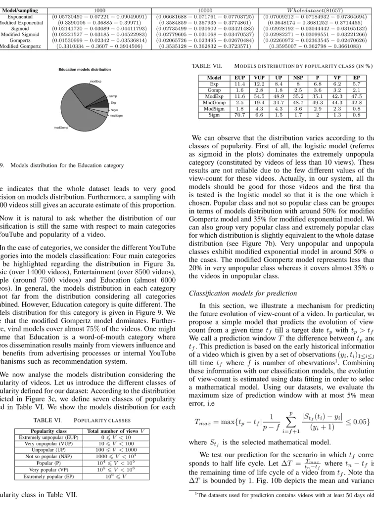
Fig. 9. Models distribution for the Education category
table indicates that the whole dataset leads to very good precision on models distribution. Furthermore, a sampling with 10000 videos still gives an accurate estimate of this proportion. Now it is natural to ask whether the distribution of our classification is still the same with respect to main categories in YouTube and popularity of a video.
In the case of categories, we consider the different YouTube categories into the models classification: Four main categories can be highlighted regarding the distribution in Figure 3a. Music (over14000videos), Entertainment (over8500videos), People (around 7500 videos) and Education (almost 6000
videos). In general, the models distribution in each category is not far from the distribution considering all categories combined. However, Education category is quite different. The models distribution for this category is given in Figure 9. We note that the modified Gompertz model dominates. Further-more, viral models cover almost75%of the videos. One might assume that Education is a word-of-mouth category where videos dissemination results mainly from viewers influence and few benefits from advertising processes or internal YouTube mechanisms such as recommendation system.
We now analyse the models distribution considering the popularity of videos. Let us introduce the different classes of popularity defined for our dataset: According to the distribution depicted in Figure 3c, we define seven classes of popularity listed in Table VI. We show the models distribution for each
TABLE VI. POPULARITY CLASSES
Popularity class Total number of viewsV
Extremely unpopular (EUP) 06V <10
Very unpopular (VUP) 106V <100
Unpopular (UP) 1006V <1000 Not so popular (NSP) 10006V <104 Popular (P) 104 6V <105 Very popular (VP) 105 6V <106
Extremely popular (EP) 106
6V
popularity class in Table VII.
TABLE VII. MODELS DISTRIBUTION BY POPULARITY CLASS(IN%)
Model EUP VUP UP NSP P VP EP
Exp 11.4 12.2 8.4 8 6.8 6.2 5.7 Gomp 1.6 2.8 1.8 2.5 3.6 3.2 2.1 ModExp 11.6 54.5 48.9 35.2 35.1 42.3 47.5 ModGomp 2.5 19.4 34.7 48.7 49.3 44.3 42.8 ModSigm 1.8 4.3 4.3 3.6 2.9 2.3 0.8 Sigm 70.7 6.6 1.5 1.7 2 1.3 0.8
We can observe that the distribution varies according to the classes of popularity. First of all, the logistic model (referred as sigmoid in the plots) dominates the extremely unpopular category (constituted by videos of less than 10 views). These results are not reliable due to the few different values of the view-count for these videos. Actually, in our system, all the models should be good for those videos and the first that is tested is the logistic model so that it is the one which is chosen. Popular class and not so popular class can be grouped in terms of models distribution with around 50% for modified Gompertz model and 35% for modified exponential model. We can also group very popular class and extremely popular class for which distribution is slightly equivalent to the whole dataset distribution (see Figure 7b). Very unpopular and unpopular classes exhibit modified exponential model in around 50% of the cases. The modified Gompertz model represents less than 20% in very unpopular class whereas it covers almost 35% of the videos in unpopular class.
Classification models for prediction
In this section, we illustrate a mechanism for predicting the future evolution of view-count of a video. In particular, we propose a simple model that predicts the evolution of view-count from a given time tf till a target datetp withtp > tf.
We call a prediction windowT the difference betweentp and tf. This prediction is based on the early historical information
of a video which is given by a set of observations(yi, ti)1≤i≤f
till time tf where f is number of obesrvations1. Combining
these information with our classification models, the evolution of view-count is estimated using data fitting in order to select a mathematical model. Using our datasets, we evaluate the maximum size of prediction window with at most 5% mean error, i.e Tmax= max{tp−tf| 1 p−f p X i=f+1 |Stf(ti)−yi| (yi+ 1) ≤0.05} whereStf is the selected mathematical model.
We test our prediction for the scenario in whichtf
corre-sponds to half life cycle. Let ∆T = Tmax
tn−tf wheretn−tf is
the remaining time of life cycle of a video fromtf. Note that
∆T is bounded by1. Fig. 10b depicts the mean and variance
TABLE VIII. MEAN AND VARIANCE OF PREDICTION WINDOW SIZE IN THE HALF LIFE SCENARIO
Model mean var number of videos
E 0.5833692 0.1504571 4132 ME 0.576914 0.1415303 25281 G 0.3435265 0.1160928 683 MG 0.4596889 0.1360676 19349 S 0.6765688 0.1544357 1030 MS 0.4625144 0.1280855 1659 E ME G MG S MS 0.0 0.2 0.4 0.6 0.8 1.0 50 days scenario Prediction windo w siz e
(a) 50 days classification
E ME G MG S MS 0.0 0.2 0.4 0.6 0.8 1.0
Half life scenario
Prediction windo
w siz
e
(b) Half life classification Fig. 10. Prediction window size according to models type
of ∆T for each identified model. Table VIII precises values of mean and variance for each model as well as the number of videos classified in the different models. Our results show that our prediction is very powerful and most models provide a prediction window that long enough within an error bound at
5%. Further we observe that our scheme can perfectly predict the evolution of view-count till the half of the remaining time of life cycle from the time of prediction.
We tested here the prediction based on a learning sequence that was half the lifetime of each video in the dataset. This allows the prediction to rely on the same amount of data independently of the real duration of the video. We next compare this to the case in which, in contrast, the learning sequence has a fixed duration of 50 days. We note that50days represent much less than half the lifetime for most videos in the data set and therefore the prediction is less accurate. The corresponding results of this scenario are depicted in Table IX and Fig. 10b. In spite of this problem we get similar results of the average prediction window for models modified Gompertz and sigmoid (Logistic).
TABLE IX. MEAN AND VARIANCE OF PREDICTION WINDOW SIZE IN THE50DAYS SCENARIO
Model mean var number of videos
E 0.1240775 0.06050271 3401 ME 0.6159881 0.1384898 21788 G 0.1861161 0.09028605 687 MG 0.2314134 0.09438778 13821 S 0.4750911 0.1083194 1137 MS 0.2082774 0.1798454 1561
It’s now natural to further investigate our prediction method in particular in case of early predictions. We slightly modify our method of calculating the prediction window size and consider values of T equal to 7 days, 15 days and 30 days. In each scenario, we fix an horizon at 3 times the observed window size. We implement two ways for computing the prediction window size. The first one is the same as in the previous method and is called the soft window. The other one
is called the hard window which is somehow pessimistic e.g. the earlier in the prediction window, the heavier is the error. Its definition is the following :
δHT =max{k≥0| 1 k k X i=0 |ST(tT+i)−yT+i| (yT+i+ 1) ≤0.05< 1 k+ 1 k+1 X i=0 |ST(tT+i)−yT+i| (yT+i+ 1) } For each window type (soft and hard) we normalise it by the size of the observed windowT. Results are given for7days,15
days and30days scenarios in Table X, Table XI and Table XII respectively. In each Table, we give fraction of videos for each model, mean for size of prediction windows (hard and soft) and fraction of videos which meet the bound effect (e.g. when the prediction window size is bounded by the horizon).
TABLE X. 7DAYS SCENARIO
Model Type Distribution (%) Hard window Hard bounded (%) Soft window Soft bounded (%)
E 66.9 m:0.6 13.5 m:0.66 15.3 ME 0.9 m:0.75 17.9 m:0.82 20 G 10.5 m:0.42 7.8 m:0.47 8.8 MG 7.9 m:0.54 10.9 m:0.61 12.7 S 11.2 m:0.97 32.9 m:1 33.8 MS 2.6 m:0.81 18.8 m:0.84 19.5 All 100 m:0.63 15.1 m:0.68 16.6
TABLE XI. 15DAYS SCENARIO
Model Type Distribution (%) Hard window Hard bounded (%) Soft window Soft bounded (%)
E 62.7 m:0.55 10.7 m:0.59 12.1 ME 1.3 m:0.9 22.2 m:0.94 23.3 G 8.4 m:0.44 7.5 m:0.47 7.9 MG 16.5 m:0.7 13.4 m:0.77 15.6 S 8.1 m:1.1 38.1 m:1.11 38.9 MS 3 m:0.94 23 m:0.98 24.5 All 100 m:0.63 13.6 m:0.67 15
TABLE XII. 30DAYS SCENARIO
Model Type Distribution (%) Hard window Hard bounded (%) Soft window Soft bounded (%)
E 52.3 m:0.5 9.5 m:0.54 10.5 ME 2.2 m:0.79 17.3 m:0.87 19.8 G 5.2 m:0.45 8.5 m:0.48 9.1 MG 30.6 m:0.68 11.6 m:0.76 14 S 5.8 m:1.1 39.9 m:1.14 40.6 MS 3.9 m:0.89 20.8 m:0.92 21.7 All 100 m:0.61 12.5 m:0.66 13.9
VI. CONCLUSION ANDFUTUREWORK
In the present work we have focused on a method for classifying view-counts dynamics of videos on YouTube. We presented different models for YouTube view-count evolution which are able to capture virality and potential population growth. Based on these models, we have developed one system for automatic classification of the YouTube videos. It aims at classify each YouTube content within one of the four categories we defined: Viral and fixed population; Viral and growing population; non-viral fixed population; and non-viral growing population. We have tested this automatic classification in a particular dataset -that has been presented and is available upon request-. Results of our experiments reveal that a reasonably small threshold of theM ERcriterion allows to classify more than 90% of the dataset, meaning that the defined models explain the observed behaviour in most of the cases.
Our future work would focus on the context of the four de-fined categories. We will analyse how other features influence the dynamic of the view-count evolution.
REFERENCES
[1] Comscore. more than 200 billion online videos viewed globally in oc-tober, http://www.comscore.com/press events/press releases/2011/12/ more than 200 billion online videos viewed globally in october. De-cember 2011.
[2] omscore danpiech. online video by the numbers, http://www.comscore.com. July 2011.
[3] N. Bailey. The Mathematical Theory of Infectious Diseases and its
Applications. Griffin, London, 1975.
[4] F. M. Bass. The relationship between diffusion rates, experience curves, and demand elasticities for consumer durable technological innovations.
The Journal of Business, 53(3):pp. 51–67, 1980.
[5] M. Cha, H. Kwak, P. Rodriguez, Y.-Y. Ahn, and S. Moon. I tube, you tube, everybody tubes: analyzing the world’s largest user generated content video system. In Proc. of ACM IMC, pages 1–14, San Diego, California, USA, October 24-26 2007.
[6] M. Cha, H. Kwak, P. Rodriguez, Y.-Y. Ahn, and S. Moon. Analyzing the video popularity characteristics of large-scale user generated content systems. IEEE/ACM Transactions on Networking, 17(5):1357 – 1370, 2009.
[7] D. Chakrabarti, Y. Wang, C. Wang, J. Leskovec, and C. Faloutsos. Epidemic thresholds in real networks. ACM Trans. Inf. Syst. Secur., 10(4):1:1–1:26, jan 2008.
[8] G. Chatzopoulou, C. Sheng, and M. Faloutsos. A First Step Towards Understanding Popularity in YouTube. In in Proc. of IEEE INFOCOM, pages 1 –6, San Diego, March 15-19 2010.
[9] X. Cheng, C. Dale, and J. Lui. Statistics and social network of youtube videos. In Proc. International Workshop on Quality of Service (IWQoS)
The Netherlands, page 229 238, June, 2008.
[10] R. Crane and D. Sornette. Viral, quality, and junk videos on YouTube: Separating content from noise in an information-rich environment. In
Proc. of AAAI symposium on Social Information Processing, Menlo
Park, California, CA, March 26-28 2008.
[11] W. E. Deming. The chi-test and curve fitting. Journal of the American
Statistical Association, 29(188):372–382, Dec 1934.
[12] A. Ganesh, L. Massoulie, and D. Towsley. The effect of network topology on the spread of epidemics. In INFOCOM 2005. 24th Annual
Joint Conference of the IEEE Computer and Communications Societies. Proceedings IEEE, volume 2, pages 1455–1466, Miami, FL, USA,
March 2005.
[13] P. Gill, M. Arlitt, Z. Li, and A. Mahanti. YouTube traffic characteriza-tion: A view from the edge. In Proc. of ACM IMC, 2007.
[14] V. Mahajan, E. Muller, and Y. Wind. New-Product Diffusion Models. International Series in Quantitative Marketing. Springer, 2000. [15] D. W. Marquardt. An algorithm for mean-squares estimation of
nonlinear parameters. Journal of the Society for Industrial and Applied
Mathematics, 11(2):431–441, jun 1963.
[16] L. A. Meyers. Contact network epidemiology: Bond percolation applied to infectious disease prediction and control. Bull. AMS, 44(1):63–86, 2007.
[17] S. Mitra, M. Agrawal, A. Yadav, N. Carlsson, D. Eager, and A. Mahanti. Characterizing web-based video sharing workloads. ACM Transactions
on the Web, 2(8):8 – 27, 2011.
[18] J. Ratkiewicz, F. Menczer, S. Fortunato, A. Flammini, and A. Vespig-nani. Traffic in Social Media II: Modeling Bursty popularity. In Proc.
of IEEE SocialCom, Minneapolis, August 20-22 2010.
[19] G. Szabo and B. A. Huberman. Predicting the Popularity of Online Content. Communications of the ACM, 53(8):80–88, aug 2010. [20] M. Zeni, D. Miorandi, and F. De Pellegrini. YOUStatAnalyzer: a tool
for analysing the dynamics of YouTube content popularity. In Proc. 7th
International Conference on Performance Evaluation Methodologies and Tools (Valuetools, Torino, Italy, December 2013), Torino, Italy,