HAL Id: hal-02104235
https://hal.archives-ouvertes.fr/hal-02104235v2
Preprint submitted on 24 Apr 2020
HAL
is a multi-disciplinary open access
archive for the deposit and dissemination of
sci-entific research documents, whether they are
pub-lished or not. The documents may come from
teaching and research institutions in France or
abroad, or from public or private research centers.
L’archive ouverte pluridisciplinaire
HAL
, est
destinée au dépôt et à la diffusion de documents
scientifiques de niveau recherche, publiés ou non,
émanant des établissements d’enseignement et de
recherche français ou étrangers, des laboratoires
publics ou privés.
Unbiased truncated quadratic variation for volatility
estimation in jump diffusion processes
Chiara Amorino, Arnaud Gloter
To cite this version:
Chiara Amorino, Arnaud Gloter. Unbiased truncated quadratic variation for volatility estimation in
jump diffusion processes. 2020. �hal-02104235v2�
Unbiased truncated quadratic variation for volatility estimation
in jump diffusion processes.
Chiara Amorino
∗, Arnaud Gloter
∗March 26, 2020
Abstract
The problem of integrated volatility estimation for an Ito semimartingale is considered under discrete high-frequency observations in short time horizon. We provide an asymptotic expansion for the integrated volatility that gives us, in detail, the contribution deriving from the jump part. The knowledge of such a contribution allows us to build an unbiased version of the truncated quadratic variation, in which the bias is visibly reduced. In earlier results to have the original truncated realized volatility well-performed the conditionβ > 1
2(2−α) onβ (that is such that ( 1
n) β
is the threshold of the truncated quadratic variation) and on the degree of jump activityαwas needed (see [21], [13]). In this paper we theoretically relax this condition and we show that our unbiased estimator achieves excellent numerical results for any couple (α,β).
L´evy-driven SDE, integrated variance, threshold estimator, convergence speed, high frequency data.
1
Introduction
In this paper, we consider the problem of estimating the integrated volatility of a discretely-observed one-dimensional Itˆo semimartingale over a finite interval. The class of Itˆo semimartingales has many applications in various area such as neuroscience, physics and finance. Indeed, it includes the stochastic Morris-Lecar neuron model [10] as well as important examples taken from finance such as the Barndorff-Nielsen-Shephard model [4], the Kou model [18] and the Merton model [23]; to name just a few.
In this work we aim at estimating the integrated volatility based on discrete observationsXt0, ..., Xtn of
the processX, withti=iTn. LetX be a solution of
Xt=X0+ Z t 0 bsds+ Z t 0 asdWs+ Z t 0 Z R\{0} γ(Xs−)zµ˜(ds, dz), t∈R+,
withW = (Wt)t≥0 a one dimensional Brownian motion and ˜µa compensated Poisson random measure. We also require the volatilityatto be an Itˆo semimartingale.
We consider here the setting of high frequency observations, i.e. ∆n := Tn → 0 as n → ∞. We
want to estimateIV := T1 RT
0 a 2
sf(Xs)ds, where f is a polynomial growth function. Such a quantity has
already been widely studied in the literature because of its great importance in finance. Indeed, taking
f ≡1, IV turns out being the so called integrated volatility that has particular relevance in measuring and forecasting the asset risks; its estimation on the basis of discrete observations of X is one of the long-standing problems.
In the sequel we will present some known results denoting byIV the classical integrated volatility, that is we are assumingf equals to 1.
When X is continuous, the canonical way for estimating the integrated volatility is to use the realized volatility or approximate quadratic variation at time T:
[X, X]nT :=
n−1
X
i=0
(∆Xi)2, where ∆Xi=Xti+1−Xti.
Under very weak assumptions onbanda(namely whenRT
0 b 2 sdsand RT 0 a 4
sdsare finite for allt∈(0, T]),
we have a central limit theorem (CLT) with rate √n: the processes √n([X, X]n
T −IV) converge in the
sense of stable convergence in law for processes, to a limit Z which is defined on an extension of the space and which conditionally is a centered Gaussian variable whose conditional law is characterized by its (conditional) variance VT := 2R
T
0 a 4
sds.
WhenX has jumps, the variable [X, X]n
T no longer converges toIV. However, there are other known
methods to estimate the integrated volatility.
The first type of jump-robust volatility estimators are theMultipower variations (cf [5], [6], [14]), which we do not explicitly recall here. These estimators satisfy a CLT with rate √n but with a conditional variance bigger than VT (so they are rate-efficient but not variance-efficient).
The second type of volatility estimators, introduced by Jacod and Todorov in [16], is based on estimating locally the volatility from the empirical characteristic function of the increments of the process over blocks of decreasing length but containing an increasing number of observations, and then summing the local volatility estimates.
Another method to estimate the integrated volatility in jump diffusion processes, introduced by Mancini in [20], is the use of thetruncated realized volatility or truncated quadratic variance (see [14], [21]):
ˆ IVnT := n−1 X i=0 (∆Xi)21{|∆Xi|≤vn},
where vn is a sequence of positive truncation levels, typically of the form (n1)β for someβ∈(0,12).
Below we focus on the estimation ofIV through the implementation of the truncated quadratic variation, that is based on the idea of summing only the squared increments of X whose absolute value is smaller than some thresholdvn.
It is shown in [13] that ˆIVnT has exactly the same limiting properties as [X, X]n
T does for someα∈[0,1)
andβ ∈[2(2−1α),12). The indexαis the degree of jump activity or Blumenthal-Getoor index
α:= inf ( r∈[0,2] : Z |x|≤1 |x|rF(dx)<∞ ) ,
whereFis a L´evy measure which accounts for the jumps of the process and it is such that the compensator ¯
µhas the form ¯µ(dt, dz) =F(z)dzdt.
Mancini has proved in [21] that, when the jumps of X are those of a stable process with index α≥1, the truncated quadratic variation is such that
( ˆIVnT −IV)∼P (1
n)
β(2−α). (1)
This rate is less than √nand no proper CLT is available in this case. In this paper, in order to estimate IV := T1 RT
0 a 2
sf(Xs)ds, we consider in particular the truncated
quadratic variation defined in the following way:
Qn:= n−1 X i=0 f(Xti)(Xti+1−Xti) 2ϕ ∆βn(Xti+1−Xti),
where ϕis aC∞ function that vanishes when the increments of the data are too large compared to the typical increments of a continuous diffusion process, and thus can be used to filter the contribution of the jumps.
We aim to extend the results proved in short time in [21] characterising precisely the noise introduced by the presence of jumps and finding consequently some corrections to reduce such a noise.
The main result of our paper is the asymptotic expansion for the integrated volatility. Compared to earlier results, our asymptotic expansion provides us precisely the limit to which nβ(2−α)(Q
n−IV) converges
when (n1)β(2−α)>√n, which matches with the conditionβ < 2(2−1α). Our work extends equation (1) (obtained in [21]). Indeed, we find
Qn−IV = Zn √ n+ ( 1 n) β(2−α)c α Z R ϕ(u)|u|1−αduZ T 0 |γ|α(X s)f(Xs)ds+oP(( 1 n) β(2−α)), where Zn L
−→ N(0,2R0Tas4f2(Xs)ds) stably with respect to X. The asymptotic expansion here above
allows us to deduce the behaviour of the truncated quadratic variation for each couple (α, β), that is a plus compared to (1).
Furthermore, providing we knowα(and if we do not it is enough to estimate it previously, see for example [28] or [24]), we can improve the performance of the truncated quadratic variation subtracting the bias due to the presence of jumps to the original estimator or taking particular functionsϕthat make the bias derived from the jump part equal to zero. Using the asymptotic expansion of the integrated volatility we also provide the rate of the error left after having applied the corrections. It derives from the Brownian increments mistakenly truncated away, when the truncation is tight.
Moreover, in the case where the volatility is constant, we show numerically that the corrections gained by the knowledge of the asymptotic expansion for the integrated volatility allows us to reduce visibly the noise for any β ∈(0,12) and α∈(0,2). It is a clear improvement because, if the original truncated quadratic variation was a well-performed estimator only if β > 2(2−1α) (condition that never holds for
α≥1), the unbiased truncated quadratic variation achieves excellent results for any couple (α, β). The outline of the paper is the following. In Section 2 we present the assumptions on the process X. In Section 3.1 we define the truncated quadratic variation, while Section 3.2 contains the main results of the paper. In Section 4 we show the numerical performance of the unbiased estimator. The Section 5 is devoted to the statement of propositions useful for the proof of the main results, that is given in Section 6. In Section 7 we give some technical tools about Malliavin calculus, required for the proof of some propositions, while other proofs and some technical results are presented in the Appendix.
2
Model, assumptions
The underlying processXis a one dimensionale Itˆo semimartingale on the space (Ω,F,(Ft)t≥0,P), where
(Ft)t≥0is a filtration, and observed at timesti=ni, fori= 0,1, . . . , n.
LetX be a solution to Xt=X0+ Z t 0 bsds+ Z t 0 asdWs+ Z t 0 Z R\{0} γ(Xs−)zµ˜(ds, dz), t∈R+, (2)
whereW = (Wt)t≥0is a one dimensional Brownian motion and ˜µa compensated Poisson random measure on which conditions will be given later.
We will also require the volatilityat to be an Itˆo semimartingale and it thus can be represented as
at=a0+ Z t 0 ˜bsds+Z t 0 ˜ asdWs+ Z t 0 ˆ asdWˆs+ Z t 0 Z R\{0} ˜ γszµ˜(ds, dz) + Z t 0 Z R\{0} ˆ γszµ˜2(ds, dz). (3)
The jumps of at are driven by the same Poisson compensated random measure ˜µ as X plus another
Poisson compensated measure ˜µ2. We need also a second Brownian motion ˆW: in the case of ”pure leverage” we would have ˆa≡0 and ˆW is not needed; in the case of ”no leverage” we rather have ˜a≡0. In the mixed case bothW and ˆW are needed.
2.1
Assumptions
The first assumption is a structural assumption describing the driving terms W,Wˆ, ˜µand ˜µ2; the sec-ond one being a set of csec-onditions on the coefficients implying in particular the existence of the various stochastic integrals involved above.
A1: The processes W and ˆW are two independent Brownian motion, µ and µ2 are Poisson random measures on [0,∞)×R associated to the L´evy processes L = (Lt)t≥0 and L2 = (L2t)t≥0 respectively, with Lt := Rt 0 R Rzµ˜(ds, dz) and L 2 t := Rt 0 R
Rzµ˜2(ds, dz). The compensated measures are ˜µ = µ−µ¯
and ˜µ2 = µ2 −µ¯2; we suppose that the compensator has the following form: ¯µ(dt, dz) := F(dz)dt, ¯
µ2(dt, dz) := F2(dz)dt. Conditions on the Levy measures F and F2 will be given in A3 and A4. The initial conditionX0,a0,W, ˆW,LandL2are independent. The Brownian motions and the L´evy processes are adapted with respect to the filtration (Ft)t≥0. We suppose moreover that there exists X, solution of
(2).
A2: The processes b, ˜b, ˜a, ˆa, ˜γ, ˆγ are bounded,γ is Lipschitz. The processes b, ˜aare c´adl´ag adapted,
γ, ˜γ and ˆγ are predictable, ˜b and ˆaare progressively measurable. Moreover it exists an Ft-measurable
random variableKtsuch that
E[|bt+h−bt|2|Ft]≤Kt|h|; ∀p≥1,E[|Kt|p]<∞.
We observe that the last condition on b holds true regardless if, for example, bt =b(Xt); b : R → R
Lipschitz.
The next assumption ensures the existence of the moments:
A3: For all q > 0, R|z|>1|z|qF(dz) < ∞ and R
|z|>1|z|
qF2(dz) < ∞. Moreover,
E[|X0|q] < ∞ and
E[|a0|q]<∞.
1. The jump coefficientγis bounded from below, that is infx∈R|γ(x)|:=γmin>0.
2. The L´evy measuresF andF2are absolutely continuous with respect to the Lebesgue measure and we denoteF(z) =F(dzdz),F2(z) =
F2(dz)
dz .
3. The L´evy measure F satisfies F(dz) = |z¯g|(1+αz) dz, where α∈(0,2) and ¯g : R→R is a continuous
symmetric nonnegative bounded function with ¯g(0) = 1.
4. The function ¯g is differentiable on {0<|z| ≤η} for some η > 0 with continuous derivative such that sup0<|z|≤η|g¯g¯0|<∞.
5. The jump coefficientγis upper bounded, i.e. supx∈R|γ(x)|:=γmax<∞.
6. The Levy measureF2 satisfies
R
R|z|
2F2(z)dz <∞.
The first and the fifth points of the assumptions here above are useful to compare size of jumps ofX and
L. The fourth point is required to use Malliavin calculus and it is satisfied by a large class of processes:
α- stable process (¯g= 1), truncated α-stable processes (¯g=τ, a truncation function), tempered stable process (¯g(z) =e−λ|z|, λ >0).
In the following, we will use repeatedly some moment inequalities for jump diffusion, which are gathered in Lemma 1 below and showed in the Appendix.
Lemma 1. Suppose that A1 - A4 hold. Then, for allt > s,
1)for allp≥2,E[|at−as|p]≤c|t−s|; for allq >0 supt∈[0,T]E[|at|q]<∞.
2) for all p≥2,p∈N,E[|at−as|p|Fs]≤c|t−s|.
3) for all p≥2,E[|Xt−Xs|p]
1
p ≤c|t−s| 1
p; for allq >0 sup
t∈[0,T]E[|Xt|q]<∞,
4) for all p≥2,p∈N,E[|Xt−Xs|p|Fs]≤c|t−s|(1 +|Xs|p).
5) for all p≥2,p∈N,suph∈[0,1]E[|Xs+h|p|Fs]≤c(1 +|Xs|p).
6) for all p >1,E[|Xtc−X c s| p]p1 ≤ |t−s|1 2 andE[|Xc t−X c s| p|F s] 1 p ≤c|t−s|12(1 +|Xs|p),
where we have denoted by Xc the continuous part of the processX, which is such that
Xtc−Xsc:= Z t s audWu+ Z t s budu.
3
Setting and main results
The processX is observed at regularly spaced timesti=i∆n= i Tn fori= 0,1, ..., n, within a finite time
interval [0, T]. We can assume, WLOG, that T = 1.
Our goal is to estimate the integrated volatilityIV := T1 RT
0 a 2
sf(Xs)ds, wheref is a polynomial growth
function. To do it, we propose the estimatorQn, based on the truncated quadratic variation introduced
by Mancini in [20]. Given that the quadratic variation was a good estimator for the integrated volatility in the continuous framework, the idea is to filter the contribution of the jumps and to keep only the intervals in which we judge no jumps happened. We use the size of the increment of the process Xti+1−Xti in
order to judge if a jump occurred or not in the interval [ti, ti+1): as it is hard for the increment of X with continuous transition to overcome the threshold ∆β
n = (1n)
β for β ≤ 1
2, we can assert the presence of a jump in [ti, ti+1) if|Xti+1−Xti|>∆ β n. We set Qn:= n−1 X i=0 f(Xti)(Xti+1−Xti) 2ϕ ∆βn(Xti+1−Xti), (4) where ϕ∆β n(Xti+1−Xti) =ϕ( Xti+1−Xti ∆βn ),
with ϕ a smooth version of the indicator function, such that ϕ(ζ) = 0 for each ζ, with |ζ| ≥ 2 and
ϕ(ζ) = 1 for eachζ, with|ζ| ≤1.
It is worth noting that, if we consider an additional constantkin ϕ(that becomesϕk∆β
n(Xti+1−Xti) =
ϕ(Xti+1−Xti
k∆βn
)), the only difference is the interval on which the function is 1 or 0: it will be 1 for|Xti+1−
Xti| ≤k∆
β
n; 0 for |Xti+1−Xti| ≥ 2k∆
β
n. Hence, for shortness in notations, we restrict the theoretical
analysis to the situation where k = 1 while, for applications, we may take the threshold level as k∆βn
3.1
Main results
The main result of this paper is the asymptotic expansion for the truncated integrated volatility. We show first of all it is possible to decompose the truncated quadratic variation, separating the con-tinuous part from the contribution of the jumps. We consider right after the difference between the truncated quadratic variation and the discretized volatility, showing it consists on the statistical error (which derives from the continuous part), on a noise term due to the jumps and on a third term which is negligible compared to the other two. From such an expansion it appears clearly the condition on (α, β) which specifies whether or not the truncated quadratic variation performs well for the estimation of the integrated volatility. It is also possible to build some unbiased estimators. Indeed, through Malliavin calculus, we identify the main bias term which arises from the presence of the jumps. We study then its asymptotic behavior and, by making it equal to zero or by removing it from the original truncated quadratic variation, we construct some corrected estimators.
We define as ˜QJn the jumps contribution present in the original estimatorQn:
˜ QJn:=nβ(2−α) n−1 X i=0 ( Z ti+1 ti Z R\{0} γ(Xs−)zµ˜(ds, dz))2f(Xti)ϕ ∆βn(Xti+1−Xti). (5) Denoting asoP((1 n)
k) a quantity such that oP((1n) k)
(1 n)k
P
→0, the following decomposition holds true:
Theorem 1. Suppose that A1 - A4 hold and that β ∈(0,12)and α∈(0,2) are given in definition (4)
and in the third point of A4, respectively. Then, as n→ ∞,
Qn= n−1 X i=0 f(Xti)(X c ti+1−X c ti) 2+ (1 n) β(2−α)Q˜J n+En= (6) = n−1 X i=0 f(Xti)( Z ti+1 ti asdWs)2+ ( 1 n) β(2−α)Q˜J n+En, (7) whereEn is both oP(( 1 n)
β(2−α))and, for each˜ >0,o
P((
1
n)
(1−αβ−˜)∧(1 2−˜)).
To show Theorem 1 here above, the following lemma will be useful. It illustrates the error we commit when the truncation is tight and therefore the Brownian increments are mistakenly truncated away.
Lemma 2. Suppose that A1 - A4 hold. Then,∀ >0,
n−1 X i=0 f(Xti)(X c ti+1−X c ti) 2(ϕ ∆βn(Xti+1−Xti)−1) =oP(( 1 n) 1−αβ−).
Theorem 1 anticipates that the size of the jumps part is (n1)β(2−α) (see Theorem 3) while the size of the Brownian increments wrongly removed is upper bounded by (n1)1−αβ−(see Lemma 2). Asβ∈(0,1
2), we can always find an >0 such that 1−αβ− > β(2−α) and therefore the bias derived from a tight truncation is always smaller compared to those derived from a loose truncation. However, as we will see, after having removed the contribution of the jumps such a small downward bias will represent the main error term ifαβ > 12.
In order to eliminate the bias arising from the jumps, we want to identify the term ˜QJ
n in details. For
that purpose we introduce
ˆ Qn:= ( 1 n) 2 α−β(2−α) n−1 X i=0 f(Xti)γ 2(X ti)d(γ(Xti)n β−1 α), (8)
where d(ζ) :=E[(S1α)2ϕ(S1αζ)]; (Stα)t≥0 is anα-stable process. We want to move from ˜QJ
n to ˆQn. The idea is to move from our process, that in small time behaves like
a conditional rescaled L´evy process, to anαstable distribution.
Proposition 1. Suppose that A1 - A4 hold. Let(Stα)t≥0 be anα-stable process. Let g be a measurable
bounded function such that kgkpol:= supx∈R(1+||g(xx)||p)<∞, for somep≥1,p≥αhence
|g(x)| ≤ kgkpol(|x|p+ 1). (9)
Moreover we denote kgk∞:= supx∈R|g(x)|. Then, for any >0,0< h <
1 2, |E[g(h−α1Lh)]−E[g(Sα 1)]| ≤Ch|log(h)| kgk∞+Ch 1 αkgk1− α p− ∞ kgk α p+ pol |log(h)|+ (10)
+Ch 1 αkgk1+ 1 p−αp+ ∞ kgk −1 p+ α p− pol |log(h)|1{α>1},
whereC is a constant independent ofh.
Proposition 1 requires some Malliavin calculus. The proof of Proposition 1 as well as some technical tools will be found in Section 7.
The previous proposition is an extension of Theorem 4.2 in [9] and it is useful whenkgk∞is large, com-pared tokgkpol. For instance, it is the case if consider the functiong(x) :=|x|21
|x|≤M forM large.
We need Proposition 1 to prove the following theorem, in which we consider the difference between the truncated quadratic variation and the discretized volatility. We make explicit its decomposition into the statistical error and the noise term due to the jumps, identified as ˆQn.
Theorem 2. Suppose that A1- A4 hold and that β∈(0,12)andα∈(0,2) are given in Definition 4 and in the third point of A4, respectively. Then, as n→ ∞,
Qn− 1 n n−1 X i=0 f(Xti)a 2 ti = Zn √ n+ ( 1 n) β(2−α)Qˆ n+En, (11) where En is always oP(( 1 n)
β(2−α)) and, adding the condition β > 1
4−α, it is also oP(( 1 n) (1−αβ−˜)∧(1 2−˜)). Moreover Zn L
−→N(0,2R0Tas4f2(Xs)ds)stably with respect to X.
We recognize in the expansion (11) the statistical error of model without jumps given byZn, whose
variance is equal to the so called quadricity. As said above, the term ˆQn is a bias term arising from the
presence of jumps and given by (8). From this explicit expression it is possible to remove the bias term (see Section 4).
The termEn is an additional error term that is always negligible compared to the bias deriving from the
jump part (1
n)
β(2−α)Qˆ
n (that is of order (n1)β(2−α) by Theorem 3 below).
The bias term admits a first order expansion that does not require the knowledge of the density of Sα.
Proposition 2. Suppose that A1 - A4 hold and that β∈(0,12) andα∈(0,2) are given in Definition 4 and in the third point of Assumption 4, respectively. Then
ˆ Qn= 1 ncα n−1 X i=0 f(Xti)|γ(Xti)| α( Z R ϕ(u)|u|1−αdu) + ˜E n, (12) with cα= ( α(1−α) 4Γ(2−α) cos(απ 2 ) ifα6= 1, α <2 1 2π if α= 1. (13) ˜ En=oP(1)and, ifα < 4 3, it is also n β(2−α)o P(( 1 n) (1−αβ−˜)∧(1 2−˜)) =o P(( 1 n) (1 2−2β+αβ−˜)∧(1−2β−˜)).
We have not replaced directly the right hand side of (12) in (11), observing that (1n)β(2−α)E˜n =En,
because (n1)β(2−α)E˜n is always oP((
1
n)
β(2−α)) but to get it is alsoo
P(( 1 n) (1−αβ−˜)∧(1 2−˜)) the additional conditionα < 43 is required.
Proposition 2 provides the contribution of the jumps in detail, identifying a main term. Recalling we are dealing with some bias, it comes naturally to look for some conditions to make it equal to zero and to study its asymptotic behaviour in order to remove its limit.
Corollary 1. Suppose that A1 - A4 hold and that α∈ (0,43), β ∈ (4−1α, (21α∧ 1
2)). If ϕ is such that R R|u| 1−αϕ(u)du= 0 then, ∀˜ >0, Qn− 1 n n−1 X i=0 f(Xti)a 2 ti = Zn √ n+oP(( 1 n) 1 2−˜), (14)
with Zn defined as in Theorem 2 here above.
It is always possible to build a functionϕfor which the condition here above is respected (see Section 4).
We have supposed α < 43 in order to say that the error we commit identifying the contribution of the jumps as the first term in the right hand side of (12) is always negligible compared to the statistical error. Moreover, taking β < 1
2α we get 1−αβ >
1
2 and therefore also the bias studied in Lemma 2 becomes upper bounded by a quantity which is roughlyoP(√1
n).
after having removed the noise derived from the presence of jumps. Taking αandβ as discussed above we have, in other words, reduced the error termEn to be oP((
1
n)
1
2−˜), which is roughly the same size as
the statistical error.
We observe that, ifα≥4
3 butγ=k∈R, the result still holds if we chooseϕsuch that
Z R u2ϕ(u)fα( 1 ku( 1 n) β−1 α)du= 0,
wherefαis the density of theα-stable process. Indeed, following (8), the jump bias ˆQnis now defined as
(1 n) 2 α−β(2−α) n−1 X i=0 f(Xti)k 2d(k nβ−1 α) = (1 n) 2 α−β(2−α) n−1 X i=0 f(Xti)k 2 Z R z2ϕ(zk(1 n) 1 α−β)fα(z)dz= = (1 n) 2 α−β(2−α) n−1 X i=0 f(Xti)k 2(1 n) 3(β−1 α) 1 k3 Z R u2ϕ(u)fα( 1 ku( 1 n) β−1 α)du= 0,
where we have used a change of variable.
Another way to construct an unbiased estimator is to study how the main bias detailed in (12) asymp-totically behaves and to remove it from the original estimator.
Theorem 3. Suppose that A1 - A4 hold. Then, asn→ ∞,
ˆ Qn →P cα Z R ϕ(u)|u|1−αdu Z T 0 |γ(Xs)|αf(Xs)ds. (15) Moreover Qn−IV = Zn √ n+ ( 1 n) β(2−α)c α Z R ϕ(u)|u|1−αdu Z T 0 |γ(Xs)|αf(Xs)ds+oP(( 1 n) β(2−α)), (16) whereZn L
−→N(0,2R0Tas4f2(Xs)ds)stably with respect toX.
It is worth noting that, in both [15] and [21], the integrated volatility estimation in short time is dealt and they show that the truncated quadratic variation has rate√nifβ > 2(2−1α).
We remark that the jump part is negligible compared to the statistic error if n−1 < n− 1
2β(2−α) and so
β > 1
2(2−α), that is the same condition given in the literature.
However, if we take (α, β) for which such a condition doesn’t hold, we can still use that we know in detail the noise deriving from jumps to implement corrections that still make the unbiased estimator well-performed (see Section 4).
We require the activity α to be known, for conducting bias correction. If it is unknown, we need to estimate it previously (see for example the methods proposed by Todorov in [28] and by Mies in [24]). Then, a question could be how the estimation error inαwould affect the rate of the bias-corrected estima-tor. We therefore assume that ˆαn =α+OP(an), for some rate sequencean. Replacing ˆαn in (16) it turns
out that the error derived from the estimation ofαdoes not affect the correction ifan(n1)β(2−α)<(n1)
1 2,
which means that an has to be smaller than (1n)
1
2−β(2−α). We recall that β ∈ (0,1
2) and α ∈ (0,2). Hence, such a condition is not a strong requirement and it becomes less and less restrictive whenαgets smaller orβ gets bigger.
4
Unbiased estimation in the case of constant volatility
In this section we consider a concrete application of the unbiased volatility estimator in a jump diffusion model and we investigate its numerical performance.
We consider our model (2) in which we assume, in addition, that the functionsaandγare both constants. Suppose that we are given a discrete sample Xt0, ..., Xtn withti=i∆n=
i
n fori= 0, ..., n.
We now want to analyze the estimation improvement; to do it we compare the classical error committed using the truncated quadratic variation with the unbiased estimation derived by our main results. We define the estimator we are going to use, in which we have clearly takenf ≡1 and we have introduced a thresholdk in the functionϕ, so it is
Qn= n−1 X i=0 (Xti+1−Xti) 2 ϕk∆β n(Xti+1−Xti). (17)
If normalized, the error committed estimating the volatility isE1:= (Qn−σ2) √
n. We start from (12) that in our case, taking into account the presence ofk, is
ˆ Qn=cαγαk2−α( Z R ϕ(u)|u|1−αdu) + ˜E n. (18)
We now get different methods to make the error smaller.
First of all we can replace (18) in (11) and so we can reduce the error by subtracting a correction term, building the new estimator Qc
n := Qn −(n1)β(2−α)cαγαk2−α(
R
Rϕ(u)|u|
1−αdu). The error committed
estimating the volatility with such a corrected estimator isE2:= (Qcn−σ2) √
n.
Another approach consists of taking a particular function ˜ϕ that makes the main contribution of ˆQn
equal to 0. We define ˜ϕ(ζ) =ϕ(ζ) +cψ(ζ), withψa C∞ function such thatψ(ζ) = 0 for eachζ,|ζ| ≥2 or|ζ| ≤1. In this way, for anyc∈R\ {0}, ˜ϕis still a smooth version of the indicator function such that
˜
ϕ(ζ) = 0 for eachζ,|ζ| ≥2 and ˜ϕ(ζ) = 1 for eachζ,|ζ| ≤1. We can therefore leverage the arbitrariness incto make the main contribution of ˆQn equal to zero, choosing ˜c:=−
R
Rϕ(u)|u|
1−αdu
R
Rψ(u)|u|
1−αdu, which is such that
R
R(ϕ+ ˜cψ(u))|u|
1−αdu= 0.
Hence, it is possible to achieve an improved estimation of the volatility by used the truncated quadratic variationQn,c :=P
n−1
i=0(Xti+1−Xti)
2(ϕ+ ˜cψ)(Xti+1−Xti
k∆βn
). To make it clear we will analyze the quantity
E3:= (Qn,c−σ2) √
n.
Another method widely used in numerical analysis to improve the rate of convergence of a sequence is the so-called Richardson extrapolation. We observe that the first term on the right hand side of (18) does not depend onnand so we can just write ˆQn= ˆQ+ ˜En. Replacing it in (11) we get
Qn=σ2+ Zn √ n + 1 nβ(2−α)Qˆ+En and Q2n=σ2+ Z2n √ 2n+ 1 2β(2−α) 1 nβ(2−α)Qˆ+E2n, where we have also used that (1
n) β(2−α)E˜
n = En. We can therefore use Qn−2
β(2−α)Q 2n
1−2β(2−α) as improved
estimator ofσ2.
We give simulation results for E1, E2 and E3 in the situation whereσ = 1. The given mean and the deviation standard are each based on 500 Monte Carlo samples. We choose to simulate a tempered stable process (that is F satisfies F(dz) = |ez|−|1+αz| ) in the case α < 1 while, in the interest of computational
efficiency, we will exhibit results gained from the simulation of a stable L´evy process in the case α≥1 (F(dz) = |z|11+α).
We have taken the smooth functionsϕandψas below:
ϕ(x) = 1 if|x|<1 e13+|x|21−4 if 1≤ |x|<2 0 if|x| ≥2 (19) ψM(x) = 0 if|x| ≤1 or|x| ≥M e 1 3+ 1 |3−x|2−4 if 1<|x| ≤3 2 e 1 |x|2−M− 5 21+ 4 4M2−9 if 3 2 <|x|< M; (20)
choosing opportunely the constantM in the definition ofψM we can make its decay slower or faster. We
observe that the theoretical results still hold even if the support of ˜ϕchanges asM changes and so it is [−M, M] instead of [-2, 2].
Concerning the constant kin the definition ofϕ, we fix it equal to 3 in the simulation of the tempered stable process, while its value is 2 in the case α >1, β = 0.2 and, in the case α >1 and β = 0.49, it increases asαandγincrease.
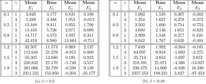
The results of the simulations are given in columns 3-6 of Table 1a for β = 0.2 and in columns 3-6 of Table 1b forβ= 0.49.
It appears that the estimation we get using the truncated quadratic variation performs worse as soon as α and γ become bigger (see column 3 in both Tables 1a and 1b). However, after having applied the corrections, the error seems visibly reduced. A proof of which lies, for example, in the comparison between the error and the root mean square: before the adjustment in both Tables 1a and 1b the third column dominates the fourth one, showing that the bias of the original estimator dominates the standard deviation while, after the implementation of our main results, we get E2 and E3 for which the bias is much smaller.
α γ Mean Rms Mean Mean E1 E1 E2 E3 0.1 1 3.820 3.177 0.831 0.189 3 5.289 3.388 1.953 -0.013 0.5 1 15.168 9.411 0.955 1.706 3 14.445 5.726 2.971 0.080 0.9 1 13.717 4.573 4.597 0.311 3 42.419 6.980 13.664 -0.711 1.2 1 32.507 11.573 0.069 2.137 3 112.648 21.279 -0.915 0.800 1.5 1 50.305 12.680 0.195 0.923 3 250.832 27.170 -5.749 3.557 1.9 1 261.066 20.729 -0.530 9.139 3 2311.521 155.950 -0.304 -35.177 (a)β= 0.2
α γ Mean Rms Mean Mean
E1 E1 E2 E3 0.1 1 1.092 1.535 0.307 -0.402 3 1.254 1.627 0.378 -0.372 0.5 1 2.503 1.690 0.754 -0.753 3 4.680 2.146 1.651 -0.824 0.9 1 2.909 1.548 0.217 0.416 3 8.042 1.767 0.620 -0.404 1.2 1 7.649 1.992 -0.944 -0.185 3 64.937 9.918 -1.692 -2.275 1.5 1 25.713 3.653 -1.697 3.653 3 218.591 21.871 -4.566 -13.027 1.9 1 238.379 14.860 -6.826 16.330 3 2357.553 189.231 3.827 -87.353 (b)β= 0.49
Table 1: Monte Carlo estimates ofE1,E2andE3from 500 samples. We have here fixedn= 700;β = 0.2 in the first table and β= 0.49 in the second one.
We observe that for α < 1, in both cases β = 0.2 and β = 0.49, it is possible to choose opportunely M (on whichψ’s decay depends) to make the errorE3 smaller thanE2. On the other hand, forα >1, the approach who consists of subtracting the jump part to the error results better than the other, since
E3 is in this case generally bigger thanE2, but to use this method the knowledge ofγ is required. It is worth noting that both the approaches used, that lead us respectively toE2 and E3, work well for any
β ∈(0,12).
We recall that, in [15], the condition found onβ to get a well-performed estimator was
β > 1
2(2−α), (21)
that is not respected in the case β = 0.2. Our results match the ones in [15], since the third column in Table 1b (where β = 0.49) is generally smaller than the third one in Table 1a (where β = 0.2). We emphasise nevertheless that, comparing columns 5 and 6 in the two tables, there is no evidence of a dependence onβ ofE2 andE3.
The price you pay is that, to implement our corrections, the knowledge ofαis request. Such corrections turn out to be a clear improvement also because for αthat is less than 1 the original estimator (17) is well-performed only for those values of the couple (α, β) which respect the condition (21) while, for
α≥1, there is noβ ∈(0,12) for which such a condition can hold. That’s the reason why, in the lower part of both Tables 1a and 1b,E1 is so big.
Using our main results, instead, we getE2andE3that are always small and so we obtain two corrections which make the unbiased estimator always well-performed without adding any requirement on αorβ.
5
Preliminary results
In the sequel, forδ≥0, we will denote asRi(∆δn) any random variable which isFti measurable and such
that, for anyq≥1,
∃c >0 : Ri(∆δn) ∆δ n Lq ≤c <∞, (22) withc independent ofi, n.
Ri represent the term of rest and have the following useful property, consequence of the just given
definition:
Ri(∆δn) = ∆ δ
nRi(∆0n). (23)
We point out that it does not involve the linearity of Ri, since the random variablesRi on the left and
on the right side are not necessarily the same but only two on which the control (22) holds with ∆δn and ∆0n, respectively.
In order to prove the main result, the following proposition will be useful. We define, fori∈ {0, ..., n−1}, ∆XiJ:= Z ti+1 ti Z R\{0} γ(Xs−)zµ˜(ds, dz) and ∆ ˜XiJ:= Z ti+1 ti Z R\{0} γ(Xti)zµ˜(ds, dz). (24)
We want to bound the error we commit moving from ∆XJ
i to ∆ ˜XiJ, denoting asoL1(∆kn) a quantity such
that Ei[|oL1(∆kn)|] =Ri(∆kn), with the notationEi[.] =E[.|Fti].
Proposition 3. Suppose that A1- A4 hold. Then
(∆XiJ)2ϕ∆β n(∆Xi) = (∆ ˜X J i ) 2ϕ ∆βn(∆ ˜X J i) +oL1(∆βn(2−α)+1)), (25) ( Z ti+1 ti asdWs)∆XiJϕ∆βn(∆Xi) = ( Z ti+1 ti asdWs)∆ ˜XiJϕ∆βn(∆ ˜X J i) +oL1(∆βn(2−α)+1)). (26)
Moreover, for each ˜ >0 andf the function introduced in the definition of Qn, n−1 X i=0 f(Xti)(∆X J i ) 2ϕ ∆βn(∆Xi) = n−1 X i=0 f(Xti)(∆ ˜X J i) 2ϕ ∆βn(∆ ˜X J i ) +oP(∆ (1−αβ−˜)∧(1 2−˜) n ), (27) n−1 X i=0 f(Xti)( Z ti+1 ti asdWs)∆XiJϕ∆βn(∆Xi) = n−1 X i=0 f(Xti)( Z ti+1 ti asdWs)∆ ˜XiJϕ∆βn(∆ ˜X J i )+oP(∆ (1−αβ−˜)∧(1 2−˜) n ). (28)
Proposition 3 will be showed in the Appendix.
In the proof of our main results, also the following lemma will be repeatedly used.
Lemma 3. Let us consider∆XJ
i and∆ ˜XiJ as defined in (24). Then
1. For eachq≥2 ∃ >0 such that
E[|∆XiJ1{|∆XJ i|≤4∆ β n}| q|F ti] =Ri(∆ 1+β(q−α) n ) =Ri(∆1+n ). (29) E[|∆ ˜XiJ1{|∆ ˜XJ i|≤4∆ β n}| q|F ti] =Ri(∆ 1+β(q−α) n ) =Ri(∆1+n ). (30)
2. For eachq≥1 we have
E[|∆XiJ1 ∆βn 4 ≤|∆X J i|≤4∆ β n |q|Ft i] =Ri(∆ 1+β(q−α) n ). (31)
Proof. Reasoning as in Lemma 10 in [2] we easily get (29). Observing that ∆ ˜XiJ is a particular case of ∆XiJ where γ is fixed, evaluated in Xti, it follows that (30) can be obtained in the same way of (29).
Using the bound on ∆XiJ obtained from the indicator function we get that the left hand side of (31) is upper bounded by c∆βqn E[1 ∆βn 4 ≤|∆XJi|≤4∆ β n |Ft i]≤∆ βq n Ri(∆1−n αβ),
where in the last inequality we have used Lemma 11 in [2] on the interval [ti, ti+1] instead of on [0, h]. From property (23) ofRi we get (31).
6
Proof of main results
We show Lemma 2, required for the proof of Theorem 1.
6.1
Proof of Lemma 2.
Proof. By the definition ofXc we have
| n−1 X i=0 f(Xti)(X c ti+1−X c ti) 2(ϕ ∆βn(∆Xi)−1)| ≤ ≤c n−1 X i=0 |f(Xti)| | Z ti+1 ti asdWs|2+| Z ti+1 ti bsds|2 |ϕ∆β n(∆Xi)−1|=:|I n 2,1|+|I n 2,2|. In the sequel the constantc may change value from line to line.
ConcerningIn
2,1, using Holder inequality we have
E[|I2n,1|]≤c n−1 X i=0 E[|f(Xti)|Ei[| Z ti+1 ti asdWs|2p] 1 pEi[|ϕ ∆βn(∆Xi)−1| q ]1q], (32)
where Ei is the conditional expectation wit respect toFti.
We now use Burkholder-Davis-Gundy inequality to get, for p1≥2,
Ei[| Z ti+1 ti asdWs|p1] 1 p1 ≤Ei[| Z ti+1 ti a2sds|p21] 1 p1 ≤Ri(∆ p1 2 n ) 1 p1 =Ri(∆ 1 2 n), (33)
where in the last inequality we have used that a2
s has bounded moments as a consequence of Lemma
1. We now observe that, from the definition of ϕwe know thatϕ∆β
n(∆Xi)−1 is different from 0 only
if |∆Xi| > ∆βn. We consider two different sets: |∆X J i | < 1 2∆ β n and |∆X J i | ≥ 1 2∆ β n. We recall that ∆Xi= ∆Xic+ ∆X J
i and so, if|∆Xi|>∆βn and|∆X J i |<
1 2∆
β
n, then it means that|∆X c
i|must be more
than 12∆βn. Using a conditional version of Tchebychev inequality we have that, ∀r >1,
Pi(|∆Xic| ≥ 1 2∆ β n)≤c Ei[|∆Xic|r] ∆βrn ≤Ri(∆ (1 2−β)r n ), (34)
wherePiis the conditional probability with respect toFti; the last inequality follows from the sixth point
of Lemma 1. If otherwise|∆XJ i | ≥ 12∆
β
n, then we introduce the setNi,n:=
n |∆Ls| ≤ 2∆β n γmin;∀s∈(ti, ti+1] o . We havePi( |∆XJ i | ≥ 12∆ β
n ∩(Ni,n)c)≤Pi((Ni,n)c), with
Pi((Ni,n)c) =Pi(∃s∈(ti, ti+1] :|∆Ls|> ∆β n 2γmin )≤c Z ti+1 ti Z ∞ ∆βn 2γmin F(z)dzds≤c∆1−n αβ, (35)
where we have used the third point of A4. Furthermore, using Markov inequality,
Pi( |∆XiJ| ≥ 1 2∆ β n ∩Ni,n)≤cEi[|∆XiJ|r1Ni,n]∆ −βr n ≤Ri(∆n−βr+1+β(r−α)) =Ri(∆1−n βα), (36)
where we have used the first point of Lemma 3, observing that 1Ni,n acts like the indicator function in
(29) (see also (219) in [2]). Now using (34), (35), (36) and the arbitrariness ofr we have
Pi(|∆Xi|>∆βn) =Pi(|∆Xi|>∆βn,|∆X J i|< 1 2∆ β n) +Pi(|∆Xi|>∆βn,|∆X J i | ≥ 1 2∆ β n)≤Ri(∆1−n αβ). (37) Takingpbig andqnext to 1 in (32) and replacing there (33) withp1= 2pand (37) we get,∀ >0,
n1−αβ−˜E[|I2n,1|]≤n1− αβ−˜c n−1 X i=1 E[|f(Xti)|Ri(∆n)Ri(∆ 1−αβ− n )]≤( 1 n) ˜ −c n n−1 X i=1 E[|f(Xti)|Ri(1)].
Now, for each ˜ >0, we can always find an smaller than it, that is enough to get that I
n 2,1
(1 n)1−αβ−˜
goes to zero inL1and so in probability. Let us now consider In
2,2. We recall thatbis uniformly bounded by a constant, therefore ( Z ti+1 ti bsds)2≤c∆2n. (38) Acting moreover on|ϕ∆β n,i
(∆Xi)−1| as we did here above it follows
n1−αβ−˜E[|I2n,2|]≤n1− αβ−˜ c n−1 X i=1 E[|f(Xti)|Ri(∆ 2 n)Ri(∆1−n αβ−)]≤( 1 n) 1+˜−c n n−1 X i=1 E[|f(Xti)|Ri(1)] and so I2n,2=oP((n1)1−αβ−˜).
6.2
Proof of Theorem 1.
We observe that, using the dynamic (2) ofX and the definition of the continuous partXc, we have that
Xti+1−Xti = (X c ti+1−X c ti) + Z ti+1 ti Z R\{0} γ(Xs−)zµ˜(ds, dz). (39)
Replacing (39) in definition (4) ofQn we have
Qn= n−1 X i=0 f(Xti)(X c ti+1−X c ti) 2+ n−1 X i=0 f(Xti)(X c ti+1−X c ti) 2(ϕ ∆βn(∆Xi)−1)+
+2 n−1 X i=0 f(Xti)(X c ti+1−X c ti)(∆X J i)ϕ∆βn(∆Xi) + n−1 X i=0 f(Xti)(∆X J i ) 2ϕ ∆βn(∆Xi) =: 4 X j=1 Ijn. (40)
Comparing (40) with (6), using also definition (5) of ˜Qn, it follows that our goal is to show that I2n+
In 3 =En, that is bothoP(∆ β(2−α) n ) and oP(∆ (1−αβ−˜)∧(1 2−˜)
n ). We have already shown in Lemma 2 that In 2 =oP(∆n1−αβ−˜). As (1−αβ−˜)∧( 1 2−˜)<1−αβ−˜andβ(2−α)<1−αβ−˜, we immediately getIn 2 =En.
Let us now consider I3n. From the definition of the process (Xtc) it is
2 n−1 X i=0 f(Xti)[ Z ti+1 ti bsds+ Z ti+1 ti asdWs]∆XiJϕ∆βn(∆Xi) =:I n 3,1+I n 3,2.
We use on I3n,1Cauchy-Schwartz inequality, (38) and Lemma 10 in [2], getting
E[|I3n,1|]≤2 n−1 X i=0 E[|f(Xti)|Ri(∆ 1+β(2−α) n ) 1 2Ri(∆2 n) 1 2]≤∆ 1 2+ β 2(2−α) n 1 n n−1 X i=0 E[|f(Xti)|Ri(1)],
where we have also used property (23) onR. We observe it is 12+β−αβ2 > 12 if and only ifβ(1−α
2)>0, that is always true. We can therefore say thatIn
3,1=oP(∆ 1 2 n) and so I3n,1=oP(∆( 1 2−˜)∧(1−αβ−˜) n ). (41) Moreover, E[|I3n,1|] ∆βn(2−α) ≤∆12−β+ αβ 2 n 1 n n−1 X i=0 E[|f(Xti)|Ri(1)], (42)
that goes to zero using the polynomial growth of f, the definition of R, the fifth point of Lemma 1. Moreover, we have observed that the exponent on ∆n is positive forβ < 12(1−1α
2)
, that is always true. ConcerningIn
3,2, we start proving thatI3n,2=oP(∆
β(2−α)
n ). From (26) in Proposition 3 we have
In 3,2 ∆βn(2−α) = 2 ∆βn(2−α) n−1 X i=0 f(Xti)∆ ˜X J iϕ∆βn(∆ ˜X J i) Z ti+1 ti asdWs+ 2 ∆βn(2−α) n−1 X i=0 f(Xti)oL1(∆ β(2−α)+1 n ). (43) By the definition ofoL1 the last term here above goes to zero in norm 1 and so in probability. The first
term of (43) can be seen as
2 ∆βn(2−α) n−1 X i=0 f(Xti)∆ ˜X J i ϕ∆βn(∆ ˜X J i )[ Z ti+1 ti atidWs+ Z ti+1 ti (as−ati)dWs]. (44)
On the first term of (44) here above we want to use Lemma 9 of [11] in order to get that it converges to zero in probability, so we have to show the following:
2 ∆βn(2−α) n−1 X i=0 Ei[f(Xti)∆ ˜X J iϕ∆βn(∆ ˜X J i) Z ti+1 ti atidWs] P −→0, (45) 4 ∆2nβ(2−α) n−1 X i=0 Ei[f2(Xti)(∆ ˜X J i ) 2ϕ2 ∆βn(∆ ˜X J i )( Z ti+1 ti atidWs) 2]−→P 0, (46) where Ei[.] =E[.|Fti].
Using the independence betweenW and Lwe have that the left hand side of (45) is
2 ∆βn(2−α) n−1 X i=0 f(Xti)Ei[∆ ˜X J iϕ∆βn(∆ ˜X J i)]Ei[ Z ti+1 ti atidWs] = 0. (47)
Now, in order to prove (46), we use Holder inequality with p big andq next to 1 on its left hand side, getting it is upper bounded by
∆−2n β(2−α) n−1 X i=0 f2(Xti)Ei[( Z ti+1 ti atidWs) 2p ]p1Ei[|∆ ˜XJ iϕ∆βn(∆ ˜X J i )| 2q ]1q ≤
≤∆−2n β(2−α) n−1 X i=0 f2(Xti)Ri(∆n)Ri(∆ 1 q+ β q(2q−α) n )≤∆1−2n β(2−α)+2β−αβ− 1 n n−1 X i=0 f2(Xti)Ri(1), (48)
where we have used (33), (30) and property (23) of R. We observe that the exponent on ∆n is positive
ifβ < 1
2−α−and we can always find an >0 such that it is true. Hence (48) goes to zero in norm 1
and so in probability.
Concerning the second term of (44), using Cauchy-Schwartz inequality and (30) we have
Ei[|∆ ˜XiJϕ∆βn(∆ ˜X J i)|| Z ti+1 ti [as−ati]dWs|]≤Ei[|∆ ˜X J iϕ∆βn(∆ ˜X J i)| 2]1 2Ei[| Z ti+1 ti [as−ati]dWs| 2]1 2 ≤ ≤Ri(∆ 1 2+ β 2(2−α) n )Ei[ Z ti+1 ti |as−ati| 2ds]1 2 ≤∆ 1 2+ β 2(2−α) n Ri(1)∆n≤∆ 3 2+ β 2(2−α) n,i Ri(1), (49)
where we have also used the second point of Lemma 1 and the property (23) ofR. Replacing (49) in the second term of (44) we get it is upper bounded in norm 1 by
∆ 1 2−β+ αβ 2 n 1 n n−1 X i=0 E[|f(Xti)|Ri(1)], (50)
that goes to zero since the exponent on ∆n is more than 0 for β < 12(1−1α 2)
, that is always true. Using (43) - (46) and (50) we get In 3,2 ∆βn(2−α) P −→0. (51)
We now want to show thatIn
3,2 is alsooP(∆
(1
2−˜)∧(1−αβ−˜)
n ).
Using (28) in Proposition 3 we get it is enough to prove that
1 ∆12−˜ n n−1 X i=0 f(Xti)[∆ ˜X J iϕ∆βn(∆ ˜X J i) Z ti+1 ti asdWs]−→P 0, (52)
where the left hand side here above can be seen as (44), with the only difference that now we have ∆
1 2−˜
n
instead of ∆βn(2−α). We have again, acting like we did in (47) and (48),
2 ∆ 1 2−˜ n n−1 X i=0 f(Xti)Ei[∆ ˜X J iϕ∆βn(∆ ˜X J i) Z ti+1 ti atidWs] P −→0 (53) and 4 ∆2(12−˜) n n−1 X i=0 Ei[f2(Xti)(∆ ˜X J i) 2 ϕ2∆β n(∆ ˜X J i)( Z ti+1 ti atidWs) 2 ]≤∆2˜n+2β−αβ− 1 n n−1 X i=0 f2(Xti)Ri(1), (54)
that goes to zero in norm 1 and so in probability. Using also (49) we have that
2 ∆ 1 2−˜ n n−1 X i=0 Ei[|f(Xti)∆ ˜X J iϕ∆βn(∆ ˜X J i) Z ti+1 ti [as−ati]dWs|]≤∆ β 2(2−α)+˜ n 1 n n−1 X i=0 |f(Xti)|Ri(1), (55)
that, again, goes to zero in norm 1 and so in probability since the exponent on ∆n is always positive.
Using (52) - (55) we getIn 3,2=oP(∆ 1 2−˜ n ) and so I3n,2=oP(∆( 1 2−˜)∧(1−αβ−˜) n ). (56)
From Lemma 2, (41), (42), (51) and (56) it follows (6).
Now, in order to prove (7), we recall the definition ofXc t: Xtc i+1−X c ti = Z ti+1 ti bsds+ Z ti+1 ti asdWs. (57)
Replacing (57) in (6) and comparing it with (7) it follows that our goal is to show that
An1+A n 2 := n−1 X i=0 f(Xti)( Z ti+1 ti bsds)2+ 2 n−1 X i=0 f(Xti)( Z ti+1 ti bsds)( Z ti+1 ti asdWs) =En.
Using (38) and property (23) ofRwe know that E[|An1|] ∆βn(2−α) ≤ 1 ∆βn(2−α) n−1 X i=0 E[|f(Xti)|Ri(∆ 2 n)]≤∆1− β(2−α) n 1 n n−1 X i=0 E[|f(Xti)|Ri(1)] (58) and E[|An1|] ∆12−˜ n ≤∆12+˜ n 1 n n−1 X i=0 E[|f(Xti)|Ri(1)], (59)
that go to zero since the exponent on ∆n is always more than 0,f has both polynomial growth and the
moment are bounded. Let us now considerAn
2. By adding and subtractingbti in the first integral, as we have already done, we
get that An2 = n−1 X i=0 ζn,i+An2,2:= 2 n−1 X i=0 f(Xti)( Z ti+1 ti btids)( Z ti+1 ti asdWs)+2 n−1 X i=0 f(Xti)( Z ti+1 ti [bs−bti]ds)( Z ti+1 ti asdWs).
Using Lemma 9 in [11], we want to show that
n−1
X
i=0
ζn,i=En (60)
and so that the following convergences hold:
1 ∆βn(2−α) n−1 X i=0 Ei[ζn,i]−→P 0 1 ∆12−˜ n n−1 X i=0 Ei[ζn,i]−→P 0; (61) 1 ∆2nβ(2−α) n−1 X i=0 Ei[ζn,i2 ] P −→0 1 ∆2( 1 2−˜) n n−1 X i=0 Ei[ζn,i2 ] P −→0. (62) We have n−1 X i=0 Ei[ζn,i] = 2 ∆βn(2−α) n−1 X i=0 f(Xti)∆nbtiEi[ Z ti+1 ti asdWs] = 0
and so the two convergences in (61) both hold. Concerning (62), using (33) we have
∆1−2n β(2−α)c n n−1 X i=0 f2(Xti)b 2 tiEi[( Z ti+1 ti asdWs)2]≤∆2−2n β(2−α) c n n−1 X i=0 f2(Xti)b 2 tiRi(1) and ∆1−2( 1 2−˜) n c n n−1 X i=0 f2(Xti)b 2 tiEi[( Z ti+1 ti asdWs)2]≤∆1+2˜n c n n−1 X i=0 f2(Xti)b 2 tiRi(1),
that go to zero in norm 1 and so in probability since ∆n is always positive. It follows (62) and so (60).
ConcerningAn2,2, using Holder inequality, (33), the assumption onbgathered in A2 and Jensen inequality it is E[|An2,2|]≤c n−1 X i=0 E[|f(Xti)|Ei[( Z ti+1 ti |bs−bti|ds) q]1qR i(∆ 1 2 n)]≤ ≤c n−1 X i=0 E[|f(Xti)|(∆ q−1 n Z ti+1 ti Ei[|bs−bti| q ]ds)1qRi(∆ 1 2 n)]≤c n−1 X i=0 E[|f(Xti)|(∆ q−1 n Z ti+1 ti ∆nds) 1 qRi(∆ 1 2 n)]. So we get E[|An2,2|] ∆βn(2−α) ≤∆ 1 q+12−β(2−α) n c n n−1 X i=0 E[|f(Xti)|Ri(1)] and (63) E[|An2,2|] ∆12−˜ n ≤∆ 1 q+˜ n c n n−1 X i=0 E[|f(Xti)|Ri(1)]. (64)
Since it holds forq≥2, the best choice is to takeq= 2, in this way we get that (63) and (64) go to 0 in norm 1, using the polynomial growth off, the boundedness of the moments, the definition ofRiand the
fact that the exponent on ∆n is in both cases more than zero, because ofβ < 2−1α.
6.3
Proof of Theorem 2
Proof. From Theorem 1 it is enough to prove that
n−1 X i=0 f(Xti)( Z ti+1 ti asdWs)2− 1 n n−1 X i=0 f(Xti)a 2 ti= Zn √ n+En, (65) and ˜ QJn= ˆQn+ 1 ∆βn(2−α) En, whereEn is alwaysoP(∆ β(2−α)
n ) and, ifβ > 4−1α, then it is alsooP(∆
(1
2−˜)∧(1−αβ−˜)
n ). We can rewrite the
last equation here above as
˜ QJn = ˆQn+oP(1) (66) and, forβ > 4−1α, ˜ QJn= ˆQn+ 1 ∆βn(2−α) oP(∆( 1 2−˜)∧(1−αβ−˜) n ). (67)
Indeed, using them and (7) it follows (11). Hence we are now left to prove (65) - (67).
Proof of (65).
We can see the left hand side of (65) as
n−1 X i=0 f(Xti)[( Z ti+1 ti asdWs)2− Z ti+1 ti a2sds] + n−1 X i=0 f(Xti) Z ti+1 ti [a2s−a2t i]ds=:M Q n +Bn. (68)
We want to show thatBn=En, it means that it is bothoP(∆ β(2−α) n ) andoP(∆ (1 2−˜)∧(1−αβ−˜) n ). We write a2s−a2ti = 2ati(as−ati) + (as−ati) 2, (69)
replacing (69) in the definition ofBn it isBn =B1n+B2n. We start by proving thatB2n =oP(∆
β(2−α)
n ).
Indeed, from the second point of Lemma 1, it is
E[|Bn2|]≤c n−1 X i=0 E[|f(Xti)| Z ti+1 ti Ei[|as−ati| 2]ds]≤c∆2 n n−1 X i=0 E[|f(Xti)|]. It follows E[|B2n|] ∆βn(2−α) ≤∆1−n β(2−α)1 n n−1 X i=0 E[|f|(Xti)] and E[|B2n|] ∆ 1 2−˜ n ≤∆ 1 2+˜ n 1 n n−1 X i=0 E[|f|(Xti)], (70)
that go to zero using the polynomial growth of f and the fact that the moments are bounded. We have also observed that the exponent on ∆n is always more than 0.
ConcerningBn
1, we recall that from (3) it follows
as−ati= Z s ti ˜budu+Z s ti ˜ audWu+ Z s ti ˆ audWˆu+ Z s ti Z R\{0} ˜ γuzµ˜(du, dz) + Z s ti Z R\{0} ˆ γuzµ˜2(du, dz)
and so, replacing it in the definition ofBn1, we getB1n:=I1n+I2n+I3n+I4n+I5n. We start consideringI1n on which we use that ˜bis bounded
E[|I1n|]≤2 n−1 X i=0 E[|f(Xti)||ati| Z ti+1 ti ( Z s ti cdu)ds]≤∆n 1 n n−1 X i=0 E[|f(Xti)||ati|]. It follows E[|I1n|] ∆βn(2−α) ≤∆1−n β(2−α)1 n n−1 X i=0 E[|f(Xti)||ati|] and (71) E[|I1n|] ∆12−˜ n ≤∆ 1 2+˜ n 1 n n−1 X i=0 E[|f(Xti)||ati|], (72)
that go to zero because of the polynomial growth of f, the boundedness of the moments and the fact that 1−β(2−α)>0.
We now act onIn
2 andI3nin the same way. ConsideringI2n, we defineζn,i:= 2f(Xti)ati
Rti+1
ti (
Rs
ti˜audWu)ds.
We want to use Lemma 9 in [11] to get that
I2n ∆βn(2−α) P −→0 and I n 2 ∆( 1 2−˜)∧(1−αβ−˜) n P −→0 (73)
and so we have to show the following :
1 ∆βn(2−α) n−1 X i=0 Ei[ζn,i]−→P 0, 1 ∆ 1 2−˜ n n−1 X i=0 Ei[ζn,i]−→P 0; (74) 1 ∆2nβ(2−α) n−1 X i=0 Ei[ζn,i2 ] P −→0, (75) 1 ∆2(12−˜) n n−1 X i=0 Ei[ζn,i2 ] P −→0. (76)
By the definition ofζn,i it isEi[ζn,i] = 0 and so (74) is clearly true. The left hand side of (75) is
∆−2n β(2−α)4 n−1 X i=0 f2(Xti)a 2 tiEi[( Z ti+1 ti ( Z s ti ˜ audWu)ds)2]. (77)
Using Fubini theorem and Ito isometry we have
Ei[( Z ti+1 ti ( Z s ti ˜ audWu)ds)2] =Ei[( Z ti+1 ti (ti+1−s)˜asdWs)2] =Ei[ Z ti+1 ti (ti+1−s2)˜a2sds]≤Ri(∆3n). (78)
Because of (78), we get that (77) is upper bounded by
∆2−2n β(2−α)1 n n−1 X i=0 f2(Xti)a 2 tiRi(1),
that converges to zero in norm 1 and so (75) follows, since 2−2β(2−α)>0 forβ < 1
2−α, that is always
true. Acting in the same way we get that the left hand side of (76) is upper bounded by
∆1+2˜n 1 n n−1 X i=0 f2(Xti)a 2 tiRi(1),
that goes to zero in norm 1. The same holds clearly forIn
3 instead ofI2n. In order to show also
In 4 ∆βn(2−α) P −→0 and I n 4 ∆(12−˜)∧(1−αβ−˜) n P −→0, (79) we define ˜ζn,i := 2f(Xti)ati Rti+1 ti ( Rs ti R
R˜γuzµ˜(du, dz))ds. We have again Ei[ ˜ζn,i] = 0 and so (74) holds
with ˜ζn,i in place of ζn,i. We now act like we did in (78), using Fubini theorem and Ito isometry. It
follows Ei[( Z ti+1 ti ( Z s ti Z R ˜ γuzµ˜(du, dz)ds)2] =Ei[( Z ti+1 ti Z R (ti+1−s)˜γszµ˜(ds, dz))2] = =Ei[ Z ti+1 ti (ti+1−s)2γ˜s2ds( Z R z2F(z)dz)]≤Ri(∆3n), (80)
having used in the last inequality the definition of ¯µ(ds, dz), the fact that R
Rz
2F(z)dz < ∞ and the boundedness of ˜γ. Replacing (80) in the left hand side of (75) and (76), with ˜ζn,iin place ofζn,i, we have
1 ∆2nβ(2−α) n−1 X i=0 Ei[ ˜ζn,i2 ]≤c∆ −2β(2−α) n n−1 X i=0 f2(Xti)a 2 tiRi(∆ 3 n)≤∆ 2−2β(2−α) n 1 n n−1 X i=0 f2(Xti)a 2 tiRi(1) and 1 ∆1−2˜n n−1 X i=0 Ei[ ˜ζn,i2 ]≤∆ 1+2˜ n 1 n n−1 X i=0 f2(Xti)a 2 tiRi(1).
Again, they converge to zero in norm 1 and thus in probability since 2−2β(2−α)>0 always holds. Therefore, we get (79). Clearly, (79) holds also withIn
the sixth point of A4 on F2 is proof of that. From (70), (71), (72), (73) and (79) it follows that
Bn=En. (81)
Concerning MQ n :=
Pn−1
i=0 ζˆn,i, Genon - Catalot and Jacod have proved in [11] that, in the continuous
framework, the following conditions are enough to get √nMnQ → N(0,2
RT 0 f 2(X s)a4sds) stably with respect to X: • Ei[ ˆζn,i] = 0; • Pn−1 i=0 Ei[ ˆζn,i2 ] P −→2RT 0 f 2(X s)a4sds; • Pn−1 i=0 Ei[ ˆζn,i4 ] P −→0; • Pn−1 i=0 Ei[ ˆζn,i(Wti+1−Wti)] P −→0; • Pn−1 i=0 Ei[ ˆζn,i( ˆWti+1−Wˆti)] P −→0.
Theorem 2.2.15 in [14] adapts the previous theorem to our framework, in which there is the presence of jumps.
We observe that the conditions here above are respected, hence
MnQ= √Zn n, whereZn n −→N(0,2 Z T 0 f2(Xs)a4sds), (82)
stably with respect toX. From (81) and (82), it follows (65).
Proof of (66).
We use Proposition 3 replacing (25) in the definition (5) of ˜QJ
n. Recalling that the convergence in norm
1 implies the convergence in probability it is clear that we have to prove the result on
nβ(2−α) n−1 X i=0 f(Xti)(∆ ˜X J i ) 2ϕ ∆βn(∆ ˜X J i ) = =nβ(2−α) n−1 X i=0 f(Xti)γ 2(X ti)∆ 2 α n( ∆ ˜XJ i γ(Xti)∆ 1 α n )2ϕ∆β n( ∆ ˜XJ i γ(Xti)∆ 1 α n γ(Xti)∆ 1 α n), (83)
where we have also rescaled the process in order to apply Proposition 1. We now define
gi,n(y) :=y2ϕ∆β
n(yγ(Xti)∆ 1 α
n), (84)
hence we can rewrite (83) as
(1 n) 2 α−β(2−α) n−1 X i=0 f(Xti)γ 2(X ti)[gi,n( ∆ ˜XiJ γ(Xti)∆ 1 α n )−E[gi,n(Sα1)]]+ +(1 n) 2 α−β(2−α) n−1 X i=0 f(Xti)γ 2(X ti)E[gi,n(S α 1)] =: n−1 X i=0 An1,i+ ˆQn, (85)
where S1α is the α-stable process at time t = 1. We want to show that Pn−1
i=0 A
n
1,i converges to zero
in probability. With this purpose in mind, we take the conditional expectation of An1,i and we apply Proposition 1 on the interval [ti, ti+1] instead of on [0, h], observing that property (9) holds ongi,n for p= 2. By the definition (84) ofgi,n, we have kgi,nk∞=Ri(∆
2(β−1 α)
n ) and kgi,nkpol=Ri(1). Replacing
them in (10) we have that
|Ei[gi,n( ∆ ˜XiJ γ(Xti)∆ 1 α n )]−E[gi,n(S1α)]| ≤c,α∆n|log(∆n)|Ri(∆ 2(β−1 α) n )+ +c,α∆ 1 α n|log(∆n)|Ri(∆ 2(β−1 α)(1−α2−) n ) +c,α∆ 1 α n|log(∆n)|Ri(∆ 2(β−1 α)(32−α2−) n )1α>1.
To getPn−1
i=0 An1,i:=oP(1), we want to use Lemma 9 of [11]. We have
n−1 X i=0 |Ei[An1,i]| ≤( 1 n) 2 α−β(2−α) n−1 X i=0 |f(Xti)||γ 2(X ti)||log(∆n)|[∆ 1+2(β−1 α) n + ∆ 1 α+(2−α−)(β− 1 α) n + +∆ 1 α+(3−α−)(β− 1 α) n 1α>1]Ri(1)≤(∆αβn + ∆ 1 α− n + ∆βn−1α>1) |log(∆n)| n n−1 X i=0 |f(Xti)||γ 2(X ti)|Ri(1), (86)
where we have used property (23). Using the polynomial growth of f, the boundedness of the moments and the fifth point of Assumption 4 in order to boundγ, (86) converges to 0 in norm 1 and so in probability since ∆αβ
n log(∆n)→0 for n→ ∞and we can always find an >0 such that ∆
1 α−
n does the same.
To use Lemma 9 of [11] we have also to show that
(1 n) 4 α−2β(2−α) n−1 X i=0 f2(Xti)γ 4(X ti)Ei[(gi,n( ∆ ˜XiJ γ(Xti)∆ 1 α n )−E[gi,n(S1α)])2] P −→0. (87)
We observe thatEi[(gi,n(
∆ ˜XJ i γ(Xti)∆ 1 α n )−E[gi,n(S1α)]) 2]≤c Ei[gi,n2 ( ∆ ˜XJ i γ(Xti)∆ 1 α n )] +cEi[E[gi,n(S1α)] 2]. Now, using equation (30) of Lemma 3, we observe it is
Ei[gi,n2 ( ∆ ˜XJ i γ(Xti)∆ 1 α n )] = ∆ −4 α n γ4(X ti) Ei[(∆ ˜XiJ) 4ϕ2 ∆βn(∆ ˜X J i)] = ∆− 4 α n γ4(X ti) Ri(∆1+n β(4−α)), (88)
where ϕacts as the indicator function. Moreover we observe that
E[gi,n(S1α)] = Z R z2ϕ(∆ 1 α−β n γ(Xti)z)fα(z)dz=d(γ(Xti)∆ 1 α−β n ), (89)
withfα(z) the density of the stable process. We now introduce the following lemma, that will be shown
in the Appendix:
Lemma 4. Suppose that Assumptions 1-4 hold. Then, for eachζn such thatζn →0and for each ˆ >0,
d(ζn) =|ζn|α−2cα
Z
R
|u|1−αϕ(u)du+o(|ζn|−ˆ+|ζn|2α−2−ˆ), (90)
wherecα has been defined in (13).
Since α1−β >0,γ(Xti)∆ 1 α−β
n goes to zero forn→ ∞and so we can takeζnasγ(Xti)∆ 1 α−β n , getting that E[gi,n(S1α)] =d(γ(Xti)∆ 1 α−β n ) =Ri(∆ (1 α−β)(α−2) n ). (91)
Replacing (88) and (91) in the left hand side of (87) we get it is upper bounded by
n−1 X i=0 Ei[(An1,i) 2] = (1 n) 4 α−2β(2−α) n−1 X i=0 f2(Xti)γ 4(X ti)(Ri(∆ 1+β(4−α) n ) +Ri(∆ 4β−4 α+2−2αβ n ))≤ ≤∆αβn ∧11 n n−1 X i=0 f2(Xti)γ 4(X ti)Ri(1), (92)
that converges to zero in norm 1 and so in probability, as a consequence of the polynomial growth of f
and the fact that the exponent on ∆n is always positive. From (86) and (92) it follows n−1 X i=0 An1,i=oP(1). (93) and so (66). Proof of (67).
We use Proposition 3 replacing (27) in definition (5) of ˜QJ
n. Our goal is to prove that
nβ(2−α) n−1 X i=0 f(Xti)(∆ ˜X J i ) 2 ϕ∆β n(∆ ˜X J i) = ˆQn+oP(∆ (1 2−2β+αβ−˜)∧(1−2β−˜) n ).
On the left hand side of the equation here above we can act like we did in (83) - (85). To get (67) we are therefore left to show that , ifβ > 4−1α, thenPn−1
i=0 A n 1,iis alsooP(∆ (1 2−2β+αβ−˜)∧(1−2β−˜) n ). To prove it,
we want to use Lemma 9 of [11], hence we want to prove the following: 1 ∆ 1 2−2β+αβ−˜ n n−1 X i=0 Ei[An1,i] P −→0 and (94) 1 ∆2( 1 2−2β+αβ−˜) n n−1 X i=0 Ei[(An1,i) 2] P −→0. (95)
Using (86) we have that, if α >1, then the left hand side of (94) is in module upper bounded by ∆βn−|log(∆n)| ∆ 1 2−2β+αβ−˜ n 1 n n−1 X i=0 |f(Xti)||γ 2(X ti)|Ri(1) = ∆ 3β−αβ−1 2+˜− n |log(∆n)| 1 n n−1 X i=0 |f(Xti)||γ 2(X ti)|Ri(1),
that goes to zero since we have chosen β > 1 4−α >
1
2(3−α). Otherwise, if α≤1, then (86) gives us that the left hand side of (94) is in module upper bounded by
∆αβ n |log(∆n)| ∆12−2β+αβ−˜ n 1 n n−1 X i=0 |f(Xti)||γ 2(X ti)|Ri(1) = ∆ 2β−1 2+˜ n |log(∆n)| 1 n n−1 X i=0 |f(Xti)||γ 2(X ti)|Ri(1),
that goes to zero because β > 4−1α >14.
Using also (92), the left hand side of (95) turns out to be upper bounded by ∆−1+4β−2αβ+2˜ n ∆αβn ∧1 1 n Pn−1 i=0 f 2(X ti)γ 4(X
ti)Ri(1), that goes to zero in norm 1 and so in probability
since we have chosenβ > 4−1α. It follows (95) and so (11).
6.4
Proof of Proposition 2
Proof. To prove the proposition we replace (90) in the definition of ˆQn. It follows that our goal is to
show that I1n+I2n:= (1 n) 2 α−β(2−α) n−1 X i=0 f(Xti)γ 2(X ti)(o(|∆ 1 α−β n γ(Xti)| −ˆ+|∆α1−β n γ(Xti)| 2α−2−ˆ)) = ˜E n,
where ˜En is alwaysoP(1) and, ifα <
4 3, it is also 1 ∆β(2n −α) oP(∆(12−˜)∧(1−αβ−˜) n ). We have thatIn
1 =oP(1) since it is upper bounded by
∆α2−1−2β+αβ−ˆ(α1−β) n 1 n n−1 X i=0 Ri(1)o(1),
that goes to zero in norm 1 and so in probability since we can always find an ˆ >0 such that the exponent on ∆n is positive.
AlsoIn
2 isoP(1). Indeed it is upper bounded by
∆ 2 α−1−2β+αβ−2( 1 α−β)+2(1−αβ)−ˆ( 1 α−β) n 1 n n−1 X i=0 Ri(1)o(1). (96)
We observe that the exponent on ∆n is 1−αβ−ˆ(α1 −β) and we can always find ˆsuch that it is more
than zero, hence (96) converges in norm 1 and so in probability. In order to show that In
1 = 1 ∆β(2n −α) oP(∆ 1 2−˜ n ) =oP(∆ 1 2−˜−β(2−α) n ) we observe that In 1 ∆12−˜−β(2−α) n ≤∆α2−1− 1 2+˜−ˆ( 1 α−β) n 1 n n−1 X i=0 Ri(1)o(1).
If α < 43 we can always find ˜ and ˆ such that the exponent on ∆n is more than zero, getting the
convergence wanted. It followsIn
1 = 1 ∆β(2n −α) oP(∆(12−˜)∧(1−αβ−˜) n ). To conclude,In 2 = 1 ∆β(2n −α) oP(∆1−αβ−˜ n ) =oP(∆ 1−2β−˜ n ). Indeed, I2n ∆1−2n β−˜ ≤∆ 2 α−1−1+αβ+˜−2( 1 α−β)+2(1−αβ)−ˆ( 1 α−β) n 1 n n−1 X i=0 Ri(1)o(1). (97)
The exponent on ∆n is 2β−αβ+ ˜−ˆ(α1−β) and so we can always find ˜and ˆsuch that it is positive. It
6.5
Proof of Corollary 1
Proof. We observe that (14) is a consequence of (12) in the case where ˆQn = 0. Moreover,β < 21α implies
that ∆1−n αβ−˜ is negligible compared to ∆
1 2−˜
n . It follows (14).
6.6
Proof of Theorem 3.
Proof. The convergence (15) clearly follows from (12). Concerning the proof of (16), we can see its left hand side as
Qn− 1 n n−1 X i=0 f(Xti)a 2 ti+ 1 n n−1 X i=0 f(Xti)a 2 ti−IV1
and so, using (11) and the definition ofIV1, it turns out that our goal is to show that 1 n n−1 X i=0 f(Xti)a 2 ti− Z 1 0 f(Xs)a2sds=oP(∆ β(2−α) n ). (98)
The left hand side of (98) is
n−1 X i=0 f(Xti) Z ti+1 ti (a2ti−a2s)ds+ n−1 X i=0 Z ti+1 ti a2s(f(Xti)−f(Xs))ds=:Bn+Rn.
Bn in the equation here above is exactly the same term we have already dealt with in the proof of
Theorem 2 (see (68)). As showed in (81) it is En and so, in particular, it is alsooP(∆
β(2−α)
n ).
OnRnwe act like we did onBn,considering this time the development up to second order of the function f, getting f(Xs) =f(Xti) +f 0(X ti)(Xs−Xti) + f00( ˜Xti) 2 (Xs−Xti) 2, (99)
where ˜Xti∈[Xti, Xs]. Replacing (99) inRn we get two terms that we denote R
1
n and R2n. On them we
can act like we did on (69). The estimations gathered in Lemma 1 about the increments ofX and of a
have the same size (see points 2 and 4) and provide onBn
2 andR2n the same upper bound:
E[|R2n|]≤c n−1 X i=0 E[|f00(Xti)| Z ti+1 ti Ei[|as||Xs−Xti| 2]ds] ≤c∆2n n−1 X i=0 E[|f00(Xti)|Ri(1)],
where we have used Cauchy Schwartz inequality and the fourth point of Lemma 1. It yields R2
n = oP(∆βn(2−α)), which is the same result found in the first inequality of (70) for the increments of a.
To deal with Rn1 we replace the dynamic of X (as done with the dynamic of a for B1n). Even if the volatility coefficient in the dynamic of X is no longer bounded, the condition sups∈[ti,ti+1]Ei[|as|]<∞
(which is true according with Lemma 1) is enough to say that (78) keep holding.
Following the method provided in the proof of Theorem 2 to show thatB1n=En we obtainR1n=En and
thereforeR1
n =oP(∆
β(2−α)
n ). It yields (98) and so the theorem is proved.
7
Proof of Proposition 1.
This section is dedicate to the proof of Proposition 1. To do it, it is convenient to introduce an adequate truncation function and to consider a rescaled process, as explained in the next subsections. Moreover, the proof of Proposition 1 requires some Malliavin calculus; we recall in what follows all the technical tools to make easier the understanding of the paper.
7.1
Localization and rescaling
We introduce a truncation function in order to suppress the big jumps of (Lt). Let τ :R→[0,1] be a
symmetric function, continuous with continuous derivative, such thatτ= 1 on|z| ≤ 1
4η andτ = 0 on
|z| ≥ 1
2η , withη defined in the fourth point of Assumption 4.
On the same probability space (Ω,F,(Ft),P) we consider the L´evy process (Lt) defined below (2) which
measure is F(dz) = |zg¯|(1+αz) 1R\{0}(z)dz, according with the third point of A4, and the truncated L´evy process (Lτt) with measure Fτ(dz) given byFτ(dz) = ¯g|(zz|)1+ατ(z)1R\{0}(z)dz. This can be done by setting
Lt :=R t
0
R
Rzµ˜(ds, dz), as we have already done, and L
τ t := Rt 0 R Rzµ˜
τ(ds, dz), where ˜µ and ˜µτ are the
compensated Poisson random measures associated respectively to
µ(A) := Z [0,1] Z R Z [0,T] 1A(t, z)µg¯(dt, dz, du), A⊂[0, T]×R, µτ(A) := Z [0,1] Z R Z [0,T] 1A(t, z)1u≤τ(z)µg¯(dt, dz, du), A⊂[0, T]×R,
forµ¯ga Poisson random measure on [0, T]×
R×[0,1] with compensator ¯µ¯g(dt, dz, du) =dt|zg¯|(1+αz) 1R\{0}(z)dzdu. By construction, the restrictions of the measures µandµτ to [0, h]×Rcoincide on the set
{(u, z) such thatu≤τ(z)}, and thus coincide on the event
Ωh:= n ω∈Ω;µ¯g([0, h]×nz∈R:|z| ≥ η 4 o ×[0,1]) = 0o. Sinceµg¯([0, h]× z∈R:|z| ≥ η
4 ×[0,1]) has a Poisson distribution with parameter
λh:= Z h 0 Z |z|≥η 4 Z 1 0 ¯ g(z) |z|1+αdu dz dt≤ch; we deduce that P(Ωch)≤c h. (100) Then we have P((Lt)t≤h6= (Lτt)t≤h)≤P(Ωch)≤c h. (101)
To prove Proposition 1 we have to rescale the process (Lt)t∈[0,1], we therefore introduce an auxiliary L´evy process (Lh
t)t∈[0,1] defined possibly on another filtered space ( ˜Ω,F,˜ ( ˜Ft),P˜) and admitting the
de-compositionLh t := Rt 0 R Rzµ˜
h(dt, dz), witht∈[0,1]; where ˜µh is a compensated Poisson random measure
˜ µh=µh−µ¯h, with compensator ¯ µh(dt, dz) =dtg¯(zh 1 α) |z|1+α τ(zh 1 α)1 R\{0}(z)dz. (102)
By construction, the process (Lht)t∈[0,1] is equal in law to the rescaled truncated process (h−
1 αLτ
ht)t∈[0,1] that coincides with (h−α1Lht)t∈[0,1] on Ωn.
7.2
Malliavin calculus
In this section, we recall some results on Malliavin calculus for jump processes. We refer to [8] for a complete presentation and to [9] for the adaptation to our framework. We will work on the Poisson space associated to the measure µh defining the process (Lht)t∈[0,1] of the previous section, assuming thathis fixed. By construction, the support of µhis contained in [0,1]×Eh, whereEh:=
n z∈R:|z|<η2 1 hα1 o , withη defined in t