arXiv:1509.03888v1 [math.OC] 13 Sep 2015
State Estimation for Genetic Regulatory Networks
with Time-Varying Delays and Reaction-Diffusion
Terms
Yuanyuan Han, Xian Zhang, Member, IEEE, Ligang Wu, Senior Member, IEEE and Yantao Wang
Abstract—This paper is concerned with the state estimation
problem for genetic regulatory networks with time-varying delays and reaction-diffusion terms under Dirichlet boundary condi-tions. It is assumed that the nonlinear regulation function is of the Hill form. The purpose of this paper is to design a state observer to estimate the concentrations of mRNA and protein through available measurement outputs. By introducing new integral terms in a novel Lyapunov–Krasovskii functional and employing Wirtinger-based integral inequality, Wirtinger’s inequality, Green’s identity, convex combination approach, and reciprocally convex combination approach, an asymptotic sta-bility criterion of the error system is established in terms of linear matrix inequalities (LMIs). The obtained stability criterion depends on the upper bounds of the delays and their derivatives. It should be highlight that if the set of LMIs are feasible, the desired observer exists and can be determined. Finally, two numerical examples are presented to illustrate the effectiveness of the proposed designed scheme.
Index Terms—Genetic regulatory networks, Reaction-diffusion
terms, State estimation, Wirtinger-based integral inequality.
I. INTRODUCTION
I
n the last decades, due to the increasing progress in genome sequencing and gene recognition, genetic regulatory net-works (GRNs) have become a significant area in biological and biomedical sciences. However, there still exists large gap between the genome sequencing and the understanding of gene functions which have become challenge problems in system biology. A great amount of experimental results show that mathematical modeling of GRNs can be a powerful tool for researching the gene regulation process and discovering complex structure of a biological organism [1]–[3]. Gener-ally, there are two basic models for GRNs: Boolean model (discrete-time model) [4], [5] and differential equation model (continuous-time model) [6]–[8]. Differential equation model describes the change rates of the concentrations of mRNAs and proteins. Furthermore, differential equation model has been most frequently utilized since it can more precisely describeY. Han, X. Zhang (Corresponding author) and Y. Wang are with the School of Mathematical Science, Heilongjiang University, Harbin 150080, China, Email: [email protected].
L. Wu is with the Space Control and Inertial Technology Research Center, Harbin Institute of Technology, Harbin, 150001, China, Email: [email protected].
This work was supported in part by the National Natural Science Foundation of China (11371006, 61174126 and 61222301), the National Natural Science Foundation of Heilongjiang Province (F201326,A201416), the Fund of Hei-longjiang Education Committee (12541603), the Fundamental Research Funds for the Central Universities (HIT.BRETIV.201303), and the Heilongjiang University Innovation Fund for Graduates (YJSCX2015-033HLJU).
the whole network and made it possible to understand the dynamic behavior of whole network in detail.
In biological systems, particularly in GRNs, stability is the most significant and essential dynamical behaviors [9]– [12]. It is related to not only the structure and function of an organism but also the strength and characteristics of the external disturbances. In addition, as it is well known, time delays caused by the slow processes of transcription and translation in real GRNs. It has been well shown from present research results that time delay may lead to instability, bifurcation or oscillation for systems [13]–[16]. However, mathematical modeling of GRNs without introducing delays will lead to wrong predictions of the concentrations of mRNAs and proteins. Therefore, the problem of stability analysis for biological systems with time delays has stirred increasing research interests and a great deal of excellent results has been reported in literature in recent decades (see, e.g., [7], [8], [17]–[22]).
In some mathematical modeling, it is implicitly assumed that the genetic regulatory systems are spatially homogeneous, namely, the concentrations of mRNA and protein are homoge-nous in space at all times. However, there are some situations in which these assumptions are not reasonable. For instance, it might be necessary to consider the diffusion of regulatory proteins from one compartment to another [1], [23]–[25]. In this situation, the general functional differential equation model can not precisely describe genetic regulatory process more or less. Hence, it is imperative to introduce reaction-diffusion terms in mathematical modeling of GRNs. To the best of authors’ knowledge, the delayed GRNs with reaction-diffusion terms are only studied in [25]–[28]. Ma et al. [27] introduced reaction-diffusion terms to GRNs for the first time and established delay-dependent asymptotic stability criteria. Based on the Lyapunov functional method, Zhou, Xu and Shen [26] investigated finite-time robust stochastic stability criteria for uncertain GRNs with time-varying delays and reaction-diffusion terms. Han and Zhang [25], [28] gradually improved Ma et al.’s results by introducing novel Lyapunov–Krasovskii functional and employing Jensen’s inequality, Wirtinger’s in-equality, Green’s identity, convex combination approach and reciprocally convex combination (RCC) approach.
In complex biological networks such as neural networks and GRNs, it is often the case that only partial information about the states of the nodes is available in the network outputs. In order to understand biological networks better, it is indispensable to estimate the states of the nodes through
available measurements. Hence, the problem of state estima-tion for biological networks has been one of the investigated dynamical behaviors in recent years [5], [29]–[33]. However, to the best of the authors’ knowledge, there is still no any published result on the state estimation problem for GRNs with time-varying delays and reaction-diffusion terms, which arouses our research interests.
Motivated by above discussion, we aim to investigate the state estimation problem for GRNs with time-varying delays and reaction-diffusion terms. By introducing new integral terms into a novel Lyapunov–Krasovskii functional and em-ploying Wirtinger-based integral inequality, Wirtinger’s in-equality, Green’s identity, convex combination approach and RCC approach, an asymptotic stability criterion of the error system is established in terms of LMIs. Thereby, a state observer is designed, and the observer gain matrices are described in terms of the solution to a set of LMIs.
The rest of the paper is organized as follows: the problem is formulated and some preliminaries are given in Section 2; in Section 3, an asymptotic stability criterion for the error system is established, and an approach to design state observer is proposed; two numerical examples are provided in Section 4; and finally, we conclude this paper in Section 5.
Notation We now set some standard notations, which will
be used in the rest of the paper.Iis the identity matrix with ap-propriate dimension,AT represents the transpose of the matrix
A. For real symmetric matricesX andY, X > Y(X ≥Y)
means thatX−Y is positive definite (positive semi-definite).Ω
is a compact set in the vector spaceRnwith smooth boundary
∂Ω. Let Ck(X, Y) be the Banach space of functions which mapX intoY and have continuousk-order derivatives. For a positive integern, lethnibe the set{1,2, . . . , n}.
II. MODEL DESCRIPTION AND PRELIMINARIES
This paper considers the following GRNs with time-varying delays and reaction-diffusion terms [25]:
∂m˜i(t, x) ∂t = Pl k=1 ∂ ∂xk Dik ∂m˜i(t, x) ∂xk −aim˜i(t, x) +Pn j=1wijgj(˜pj(t−σ(t), x)) +qi, ∂p˜i(t, x) ∂t = Pl k=1 ∂ ∂xk D∗ik∂p˜i(t, x) ∂xk −cip˜i(t, x) +bim˜i(t−τ(t), x), (1) where i ∈ hni, x = col(x1, x2, . . . , xl) ∈ Ω ⊂ Rl, Ω = {x |xk| ≤ Lk, k ∈ hli}, Lk is a given constant; Dik > 0 andD∗
ik >0denote the diffusion rate matrices; m˜i(t, x)and
˜
pi(t, x) are the concentrations of mRNA and protein of the
ith node, respectively;ai andci are degradation rates of the mRNA and protein, respectively; bi represents the translation rate;W := [wij]∈Rn×nis the coupling matrix of the genetic networks, which is defined as follows:
wij=
γij, ifj is an activator of genei,
0, if there is no link from genej toi,
−γij, ifj is a repressor of genei,
hereγij is the dimensionless transcriptional rate of transcrip-tion factor j to genei;gj represents the feedback regulation
function of protein on transcription, which is the monotonic function in Hill form, i.e.,gj(s) = s
H
1+sH, whereH is the Hill
coefficient;qi= Σj∈Iiγij,Iiis the set of all the nodes which
are repressors of genei;σ(t)andτ(t)are time-varying delays satisfying
0≤τ(t)≤τ , τ˙(t)≤µ1,
0≤σ(t)≤σ, σ˙(t)≤µ2, (2)
whereτ,σ,µ1 andµ2 are non-negative real numbers.
The initial conditions associated with GRN (1) are given as follows:
˜
mi(s, x) =φi(s, x), x∈Ω, s∈[−d,0], i∈ hni,
˜
pi(s, x) =φ∗i(s, x), x∈Ω, s∈[−d,0], i∈ hni,
whered= max{σ, τ}, andφi(s, x),φ∗i(s, x)∈C1([−d,0]×
Ω,R).
In this paper, the following type of boundary conditions (Dirichlet boundary conditions) is considered:
˜
mi(t, x) = 0, x∈∂Ω, t∈[−d,+∞),
˜
pi(t, x) = 0, x∈∂Ω, t∈[−d,+∞). Now, we assume that
m∗(x) := col(m∗1(x), m∗2(x), . . . , m∗n(x))
and
p∗(x) := col(p∗1(x), p∗2(x), . . . , p∗n(x)) are the unique equilibrium solution of GRN (1), that is,
0 = Pl k=1 ∂ ∂xk Dk ∂m∗i(x) ∂xk −aim∗i(x) +Pn j=1wijgj(p∗j(x)) +qi, 0 = Pl k=1 ∂ ∂xk D∗k∂p ∗ i(x) ∂xk −cip∗i(x) +bim∗i(x) fori∈ hni. Obviously, the transformations,m¯i = ˜mi−m∗i and
¯
pi= ˜pi−p∗i,i∈ hni, transform GRN (1) into the following matrix form: ∂m¯(t, x) ∂t = Pl k=1 ∂ ∂xk Dk ∂m¯(t, x) ∂xk −Am¯(t, x) +W f(¯p(t−σ(t), x)), ∂p¯(t, x) ∂t = Pl k=1 ∂ ∂xk D∗k∂p¯(t, x) ∂xk −Cp¯(t, x) +Bm¯(t−τ(t), x), (3) where A= diag(a1, a2, . . . , an), C= diag(c1, c2, . . . , cn), B = diag(b1, b2, . . . , bn), Dk= diag(D1k, D2k, . . . , Dnk), D∗k= diag(D∗1k, D2∗k, . . . , Dnk∗ ), ¯ m(t, x) = col( ¯m1(t, x),m¯2(t, x), . . . ,m¯n(t, x)), ¯ p(t, x) = col(¯p1(t, x),p¯2(t, x), . . . ,p¯n(t, x)), f(¯p(t−σ(t), x)) = col(f1(¯p1(t−σ(t), x)),· · ·, fn(¯pn(t−σ(t), x))), fi(¯pi(t−σ(t), x)) =gi(¯pi(t−σ(t), x)+p∗i)−gi(p∗i), i∈ hni.
Because of the complexity of GRN (3), it is normally of the case that only partial information about the states of the nodes is available in the network outputs. In order to obtain the true state of (3), it becomes necessary to estimate the states of the nodes through network measurements. The available measurements are given as follows:
zm(t, x) =Mm¯(t, x),
zp(t, x) =Np¯(t, x),
(4) where zm(t, x) and zp(t, x) are the actual measurement outputs, and M and N are known constant matrices with appropriate dimensions.
To estimate the states of GRN (3) through available mea-surement outputs in (4), we construct the following state observer: ∂mˆ(t, x) ∂t = Pl k=1 ∂ ∂xk Dk ∂mˆ(t, x) ∂xk −Amˆ(t, x) +W f(ˆp(t−σ(t), x)) +K1[zm(t, x)−Mmˆ(t, x)], ∂pˆ(t, x) ∂t = Pl k=1 ∂ ∂xk D∗k∂pˆ(t, x) ∂xk −Cpˆ(t, x) +Bmˆ(t−τ(t), x) +K2[zp(t, x)−Npˆ(t, x)], (5) wheremˆ(t, x)andpˆ(t, x)are the estimations of m(t, x)and
p(t, x), respectively, and K1 and K2 are the observer gain
matrices to be designed later.
The initial conditions for the state observer (5) are assumed to be ( ˆmi(t, x),pˆi(t, x)) = (φi(s, x), φ∗i(s, x)).
Our aim is to find suitable observer gains K1 and K2,
so that mˆ(t, x)andpˆ(t, x), respectively, approach to m(t, x)
and p(t, x) as t → +∞. Let the error state vectors be
m(t, x) = ¯m(t, x)−mˆ(t, x)and p(t, x) = ¯p(t, x)−pˆ(t, x). Then it follows from (3), (4) and (5) that
∂m(t, x) ∂t = Pl k=1 ∂ ∂xk Dk ∂m(t, x) ∂xk −(A+K1M)m(t, x) +Wf¯(p(t−σ(t), x)), ∂p(t, x) ∂t = Pl k=1 ∂ ∂xk D∗k∂p(t, x) ∂xk −(C+K2N)p(t, x) +Bm(t−τ(t), x), (6) where ¯ f(p(t−σ(t), x)) =f(¯p(t−σ(t), x))−f(ˆp(t−σ(t), x)).
From the relationship among f¯i, fi andgi, one can easily obtain that ¯ fi(0) = 0,0≤ ¯ fi(y) y ≤ξi,∀y∈R, y6= 0, i∈ hni, namely, ¯ f(0) = 0,f¯T(z)( ¯f(z)−Kz)≤0,∀z∈Rn, (7) whereK= diag(ξ1, ξ2, . . . , ξn)>0.
In this paper, we assume that error system (6) satisfies Dirichlet boundary conditions:
mi(t, x) = 0, x∈∂Ω, t∈[−d,+∞),
pi(t, x) = 0, x∈∂Ω, t∈[−d,+∞).
We introduce the following lemmas which play key roles in obtaining the main results of this paper.
Lemma 1 (Jensen’s Inequality): [34], [35] For any con-stant matrix MT = M > 0 of appropriate dimension, any scalars a and b with a < b, and a vector function
w : [a, b] → Rn such that the integrals concerned are well defined, then the following inequality holds:
Z b a w(s)ds !T M Z b a w(s)ds ! ≤(b−a) Z b a wT(s)M w(s)ds, Rb a Rb θ w(s)dsdθ T MRb a Rb θ w(s)dsdθ ≤ (b−2a)2Rb a Rb θwT(s)M w(s)dsdθ.
Lemma 2 (Wirtinger-based Integral Inequality): [36] For given a symmetric positive definite matrix Q ∈ Rn×n, and a differentiable function ω : [a, b] → Rn, the following inequality holds: Z b a ˙ wT(u)Qw˙(u)du≥ 1 b−a Ω0 Ω1 T ˜ Q Ω0 Ω1 ,
whereQ˜ = diag(Q,3Q),Ω0=w(b)−w(a)and
Ω1=w(b) +w(a)− 2 b−a Z b a w(u)du.
Lemma 3 (Wirtinger’s Inequality): [37] Assume that the functionf ∈C1([a, b],Rn)satisfies f(a) =f(b) = 0. Then
Z b a f2(v)dv≤ (b−a) 2 π2 Z b a [f′(v)]2dv.
Lemma 4: [25] Let N1 > 0 and N2 > 0 be a pair of
diagonal matrices. Then the states of (6) satisfy
R Ω ∂mT(s,x) ∂t N1 Pl k=1 ∂x∂k Dk∂m∂x(t,xk ) dx = R Ωm T(t, x)N 1Plk=1∂x∂k h Dk∂x∂k ∂m(t,x) ∂t i dx, R Ω ∂pT(s,x) ∂t N2 Pl k=1∂x∂k D∗ k ∂p(t,x) ∂xk dx = R ΩpT(t, x)N2 Pl k=1 ∂x∂k h D∗ k∂x∂k ∂p(t,x) ∂t i dx.
Lemma 5 (RCC Lemma): [38] Letf1, f2, . . . , fN :D→R have positive finite values, where D is open subset of Rm. Then the RCC offi overDsatisfies
min{αi:αi>0,Piαi=1} P i 1 αifi(t) = P ifi(t) + maxgi,j(t) P i6=jgi,j(t) subject to gij:Rm→R, gj,i(t) =gi,j(t), fi(t) gi,j(t) gi,j(t) fj(t) ≥0.
III. OBSERVER DESIGN
In this section, we will design a state observer (5) for GRN (3), that is, find a pair of observer gain matrices K1 andK2
such that the trivial solution of system (6) is asymptotically stable under Dirichlet boundary conditions. For this end, we define e0= 014n×n, ei= col(0n×(i−1)n, In,0n×(n−i)n)T, i∈ h14i, ϕ(t, s, x) = col m(s, x), Z t t−τ¯ m(s, x)ds , ψ(t, s, x) = col p(s, x), Z t t−σ¯ p(s, x)ds , ς(t, x) = col(m(t, x), m(t−τ , x), m(t−τ(t), x), p(t, x) p(t−σ, x), p(t−σ(t), x),f¯(p(t, x)), ¯ f(p(t−σ(t), x)),∂m∂t(t,x),∂p(∂tt,x), 1 τ(t) Rt t−τ(t)m(s, x)ds, 1 τ−τ(t) Rt−τ(t) t−τ m(s, x)ds, 1 σ(t) Rt t−σ(t)p(s, x)ds, 1 σ−σ(t) Rt−σ(t) t−σ p(s, x)ds).
Theorem 1: For given scalars τ, σ, µ1 and µ2 satisfying
(2), the trivial solution of error system (6) under Dirichlet boundary conditions is asymptotically stable if there exist matrices QTi =Qi >0 (i ∈ h5i), RTj =Rj >0 (j ∈ h4i),
MT
j =Mj >0 (j ∈ h2i), diagonal matricesPj >0,Λj>0
(j ∈ h2i), and matrices G1, G2,W1 and W2 of appropriate
sizes, such that the following LMIs hold for τ ∈ {0,τ¯} and
σ∈ {0,¯σ}: ˆ Rj:= ˜ Rj Gj GT j R˜j ≥0, j∈ h2i, (8) Φ(τ, σ) = Φ0+Φ1+Φ2(τ, σ)+Φ3+Φ4(τ, σ)+Φ5(τ, σ)<0, (9) where Φ0= −2e7Λ1eT7 +e4Λ1Ke7T+e7KΛ1e4T −2e8Λ2eT8 +e6KΛ2eT8 +e8Λ2Ke6T −e9(P1A+W1M)eT1 −e1(P1A+W1M)TeT9 +e9P1W eT8 +e8WTP1eT9 −2e9P1eT9 −e10(P2C+W2N)eT4 −e4(P2C+W2N)TeT10+e10P2BeT3 +e3BTP2eT10−2e10P2eT10, Φ1= −0.5π2e1P1DLe1T −2e1(P1A+W1M)eT1 +e1P1W eT8 +e8WTP1eT1 −0.5π2e 4P2D∗LeT4 −2e4(P2C+W2N)eT4 +e4P2BeT3 +e3BTP2eT4, Φ2(τ, σ) = e1Q1eT1 −(1−µ1)e3Q1eT3 +e4Q3eT4 −(1−µ2)e6Q3eT6 +∆1Q2∆T1 +τ(∆1Q2∆T2 + ∆2Q2∆T1) −∆3Q2∆T3 −τ(∆3Q2∆T2 + ∆2Q2∆T3) +∆4Q2∆T6 + ∆6Q2∆T4 +τ(∆5Q2∆T6 + ∆6Q2∆T5) + Θ1Q4ΘT1 +σ(Θ1Q4ΘT2 + Θ2Q4ΘT1)−Θ3Q4ΘT3 −σ(Θ3Q4ΘT2 + Θ2Q4ΘT3) + Θ4Q4ΘT6 +Θ6Q4ΘT4 +σ(Θ5Q4ΘT6 + Θ6Q4ΘT5), Φ3=e7Q5eT7 −(1−µ2)e8Q5eT8, Φ4(τ, σ)= Φ41−Φ42(τ)−Φ43(σ) −[∆7 ∆8] ˆR1[∆7 ∆8]T −[Θ7 Θ8] ˆR2[Θ7 Θ8]T, Φ41= ¯τ2e9R1eT9 + ¯σ2e10R2e10T + ¯τ2e1R3eT1 + ¯σ2e4R4eT4, Φ42(τ) = ¯τ(¯τ−τ)e12R3eT12+ ¯τ τ e11R3eT11, Φ43(τ) = ¯σ(¯σ−σ)e14R4eT14+ ¯σσe13R4eT13, Φ5(τ, σ) = Φ51−Φ52−Φ53 −(τ−ττ)∆8M˜1∆T8 − (σ−σ) σ Θ8M˜2Θ T 8, Φ51= ¯ τ2 2 e9M1e T 9 + ¯ σ2 2 e10M2e T 10, Φ52= (e1−e11)M1(e1−e11)T +(e3−e12)M1(e3−e12)T, Φ53= (e4−e13)M2(e4−e13)T +(e6−e14)M2(e6−e14)T, ∆1= [e1 τ e¯ 12], ∆2= [e0 e11−e12], ∆3= [e2 τ e¯ 12], ∆4= [¯τ e12 τ¯2e12], ∆5= [e11−e12 ¯τ(e11−e12)], ∆6= [e0 e1−e2], ∆7= [e3−e2 e3+e2−2e12], ∆8= [e1−e3 e1+e3−2e11], Θ1= [e4 σe¯ 14], Θ2= [e0 e13−e14], Θ3= [e5 σe¯ 14], Θ4= [¯σe14 σ¯2e14], Θ5= [e13−e14 σ¯(e13−e14)], Θ6= [e0 e4−e5], Θ7= [e6−e5 e6+e5−2e14], Θ8= [e4−e6 e4+e6−2e13], ˜ R1= diag(R1,3R1), R˜2= diag(R2,3R2), ˜ M1= 1 ¯ τdiag(M1,3M1), M˜2= 1 ¯ σdiag(M2,3M2), DL= diag l X k=1 D1k L2 k , l X k=1 D2k L2 k , . . . , l X k=1 Dnk L2 k ! ,
DL∗ = diag l X k=1 D∗ 1k L2k , l X k=1 D∗ 2k L2k , . . . , l X k=1 D∗ nk L2k ! ,
and Lk, Dik, Dik∗, A, B, C, W and K are the same with previous ones.
Moreover, the observer gain matrices are given by K1 =
P1−1W1 andK2=P2−1W2.
Proof: Construct a Lyapunov-Krasovskii functional for
error system (6) as follows:
V(t, m, p) = 5 X i=1 Vi(t, m, p), where V1(t, m, p) =RΩmT(t, x)P1m(t, x)dx +R Ωp T(t, x)P 2p(t, x)dx +Pl k=1 R Ω ∂mT(t,x) ∂xk P1Dk ∂m(t,x) ∂xk dx +Pl k=1 R Ω ∂pT(t,x) ∂xk P2D ∗ k ∂p(t,x) ∂xk dx, V2(t, m, p) =RΩRtt−τ(t)mT(s, x)Q1m(s, x)dsdx +R Ω Rt t−τϕ T(t, s, x)Q 2ϕ(t, s, x)dsdx +R Ω Rt t−σ(t)p T(s, x)Q 3p(s, x)dsdx +R Ω Rt t−σψ T(t, s, x)Q 4ψ(t, s, x)dsdx, V3(t, m, p) = Z Ω Z t t−σ(t) ¯ fT(p(s, x))Q5f¯(p(s, x))dsdx, V4(t, m, p) =τRΩR−0τRtt+θ∂m T(s,x) ∂s R1 ∂m(s,x) ∂s dsdθdx +σR Ω R0 −σ Rt t+θ ∂pT(s,x) ∂s R2 ∂p(s,x) ∂s dsdθdx +τR Ω R0 −τ Rt t+θm T(s, x)R 3m(s, x)dsdθdx +σR Ω R0 −σ Rt t+θp T(s, x)R 4p(s, x)dsdθdx, V5(t, m, p) =RΩR 0 −τ R0 θ Rt t+λ ∂mT(s,x) ∂s M1 ∂m(s,x) ∂s dsdλdθdx R Ω R0 −σ R0 θ Rt t+λ ∂pT(s,x) ∂s M2 ∂p(s,x) ∂s dsdλdθdx. Taking the time derivatives of Vi(t, m, p) (i∈ h5i)along the trajectory of error system (6) yields
∂ ∂tV1(t, m, p) = 2R Ωm T(t, x)P 1 h Pl k=1 ∂x∂k Dk∂m∂x(t,xk ) −(A+K1M)m(t, x) +Wf¯(p(t−σ(t), x)) i dx +2R ΩpT(t, x)P2 h Pl k=1 ∂x∂k D∗ k ∂p(t,x) ∂xk −(C+K2N)p(t, x) +Bm(t−τ(t), x) i dx +2Pl k=1 R Ω ∂mT(t,x) ∂xk P1Dk ∂ ∂xk( ∂m(t,x) ∂t )dx +2Pl k=1 R Ω ∂pT(t,x) ∂xk P2D ∗ k ∂ ∂xk( ∂p(t,x) ∂t )dx, (10) ∂ ∂tV2(t, m, p) = R ΩmT(t, x)Q1m(t, x)dx −(1−τ˙(t))R Ωm T(t−τ(t), x)Q 1m(t−τ(t), x)dx +R Ωp T(t, x)Q 3p(t, x)dx −(1−σ˙(t))R Ωp T(t−σ(t), x)Q 3p(t−σ(t), x)dx +R ΩϕT(t, t, x)Q2ϕ(t, t, x)dx −R ΩϕT(t, t−τ , x)Q2ϕ(t, t−τ , x)dx +2R Ω Rt t−τϕ T(t, s, x)Q 2∂ϕ(∂tt,s,x)dsdx +R ΩψT(t, t, x)Q4ψ(t, t, x)dx −R ΩψT(t, t−σ, x)Q4ψ(t, t−σ, x)dx, +2R Ω Rt t−σψT(t, s, x)Q4 ∂ψ(t,s,x) ∂t dsdx ≤ R ΩςT(t, x)Φ2(τ(t), σ(t))ς(t, x)dx, (11) ∂ ∂tV3(t, m, p) =−(1−σ˙(t))R Ωf¯ T(p(t−σ(t), x))Q 5f¯(p(t−σ(t), x))dx +R Ωf¯ T(p(t, x))Q 5f¯(p(t, x))dx ≤R ΩςT(t, x)Φ3ς(t, x)dx, (12) ∂ ∂tV4(t, m, p) = τ 2R Ω ∂mT(t,x) ∂t R1 ∂m(t,x) ∂t dx −τR Ω Rt t−τ ∂mT(s,x) ∂s R1 ∂m(s,x) ∂s dsdx +σ2R Ω ∂pT(t,x) ∂t R2 ∂p(t,x) ∂t dx −σR Ω Rt t−σ ∂pT(s,x) ∂s R2 ∂p(s,x) ∂s dsdx +τ2R Ωm T(t, x)R 3m(t, x)dx −τR Ω Rt t−τm T(s, x)R 3m(s, x)dsdx +σ2R Ωp T(t, x)R 4p(t, x)dx −σR Ω Rt t−σp T(s, x)R 4p(s, x)dsdx, (13) ∂ ∂tV5(t, m, p) = τ2 2 R Ω ∂mT(t,x) ∂t M1 ∂m(t,x) ∂t dx −R Ω R0 −τ Rt t+θ ∂mT(s,x) ∂s M1 ∂m(s,x) ∂s dsdθdx +σ2 2 R Ω ∂pT(t,x) ∂t M2 ∂p(t,x) ∂t dx −R Ω R0 −σ Rt t+θ ∂pT(s,x) ∂s M2 ∂p(s,x) ∂s dsdθdx. (14) From Green formula, Dirichlet boundary conditions and Lemma 3, we have 2Pl k=1 R ΩmT(t, x)P1 ∂ ∂xk Dk∂m∂x(t,xk ) dx = 2Pl k=1 R Ω ∂ ∂xk mT(t, x)P1Dk∂m∂x(t,xk ) dx −2Pl k=1 R Ω ∂mT(t,x) ∂xk P1Dk ∂m(t,x) ∂xk dx = 2Pl k=1 R ∂Ω mT(t, x)P 1Dk∂m∂x(t,xk ) l k=1·nds −2Pl k=1 R Ω ∂mT(t,x) ∂xk P1Dk ∂m(t,x) ∂xk dx = −2Pl k=1 R Ω ∂mT(t,x) ∂xk P1Dk ∂m(t,x) ∂xk dx ≤ −π22R ΩmT(t, x)P1DLm(t, x)dx, (15)
where mT(t, x)P 1Dk∂m∂x(t,xk ) l k=1 = mT(t, x)P 1D1∂m∂x(t,x) 1 , . . . , m T(t, x)P 1Dl∂m∂x(t,xl ) . Similarly, 2Pl k=1 R Ωp T(t, x)P 2∂x∂k D∗ k ∂p(t,x) ∂xk dx ≤ −π2 2 R Ωp T(t, x)P 2DL∗p(t, x)dx. (16)
The combination of (10), (15) and (16) gives ∂ ∂tV1(t, m, p) = 2R ΩmT(t, x)P1 h −π2 4 DLm(t, x) −(A+K1M)m(t, x) +Wf¯(p(t−σ(t), x))dx +2R ΩpT(t, x)P2 h −π2 4 D ∗ Lp(t, x) −(C+K2N)p(t, x) +Bm(t−τ(t), x)] dx +2Pl k=1 R Ω ∂mT(t,x) ∂xk P1Dk ∂ ∂xk( ∂m(t,x) ∂t )dx +2Pl k=1 R Ω ∂pT(t,x) ∂xk P2D ∗ k ∂ ∂xk( ∂p(t,x) ∂t )dx = R ΩςT(t, x)Φ1ς(t, x)dx +2Pl k=1 R Ω ∂mT(t,x) ∂xk P1Dk ∂ ∂xk( ∂m(t,x) ∂t )dx +2Pl k=1 R Ω ∂pT(t,x) ∂xk P2D ∗ k∂x∂k( ∂p(t,x) ∂t )dx. (17) Note that the second term on the right of (13) can be written as: −τR Ω Rt t−τ ∂mT(s,x) ∂s R1 ∂m(s,x) ∂s dsdx = −τR Ω Rt−τ(t) t−τ ∂mT(s,x) ∂s R1 ∂m(s,x) ∂s dsdx −τR Ω Rt t−τ(t) ∂mT(s,x) ∂s R1 ∂m(s,x) ∂s dsdx. (18)
Applying Lemma 2, one can obtain that −τR Ω Rt−τ(t) t−τ ∂mT(s,x) ∂s R1 ∂m(s,x) ∂s dsdx ≤ − τ τ−τ(t) R Ως T(t, x)∆ 7R˜1∆T7ς(t, x)dx and −τR Ω Rt t−τ(t) ∂mT(s,x) ∂s R1 ∂m(s,x) ∂s dsdx ≤ − τ τ(t) R ΩςT(t, x)∆8R˜1∆8ς(t, x)dx. (19)
This, together with (8), (18) and Lemma 5, implies that −τR Ω Rt t−τ ∂mT(s,x) ∂s R1 ∂m(s,x) ∂s dsdx ≤ −R Ως T(t, x)[∆ 7 ∆8] ˆR1[∆7 ∆8]Tς(t, x)dx. (20) Similarly, −σR Ω Rt t−σ ∂pT(s,x) ∂s R2 ∂p(s,x) ∂s dsdx ≤ −R ΩςT(t, x)[ΘT7 Θ8] ˆR2[ΘT7 Θ8]Tς(t, x)dx. (21)
On the other hand, by Lemma 1, it yields −τR Ω Rt t−τm T(s, x)R 3m(s, x)dsdx =−τR Ω Rt−τ(t) t−τ m T(s, x)R 3m(s, x)dsdx −τR Ω Rt t−τ(t)mT(s, x)R3m(s, x)dsdx ≤ −τ−ττ(t)R Ω Rt−τ(t) t−τ m T(s, x)dsR 3Rt −τ(t) t−τ m(s, x)dsdx − τ τ(t) R Ω Rt t−τ(t)mT(s, x)dsR3 Rt t−τ(t)mT(s, x)dsdx ≤ −R ΩςT(t, x)Φ42(τ(t))ς(t, x)dx. (22) In the same way,
−σR Ω Rt t−σp T(s, x)R 4p(s, x)dsdx ≤ −R Ως T(t, x)Φ 43(σ(t))ς(t, x)dx. (23) Combining (13), (20)-(23) yields ∂ ∂tV4(t, m, p)≤ R Ως T(t, x)Φ 4(τ(t), σ(t))ς(t, x)dx. (24) The second term on the right of (14) can be divided into three parts: −R Ω R0 −τ Rt t+θ ∂mT(s,x) ∂s M1 ∂m(s,x) ∂s dsdθdx = −R Ω R0 −τ(t) Rt t+θ ∂mT(s,x) ∂s M1 ∂m(s,x) ∂s dsdθdx −R Ω R−τ(t) −τ Rt−τ(t) t+θ ∂mT(s,x) ∂s M1 ∂m(s,x) ∂s dsdθdx −(τ−τ(t))R Ω Rt t−τ(t) ∂mT(s,x) ∂s M1 ∂m(s,x) ∂s dsdx. (25) By using Lemma 1, we can estimate the following inequalities
−R Ω R0 −τ(t) Rt t+θ ∂mT(s,x) ∂s M1 ∂m(s,x) ∂s dsdθdx −R Ω R−τ(t) −τ Rt−τ(t) t+θ ∂mT(s,x) ∂s M1 ∂m(s,x) ∂s dsdθdx ≤ − 2 τ(t)2 R Ω R0 −τ(t) Rt t+θ ∂mT(s,x) ∂s dsdθdxM1 ×R0 −τ(t) Rt t+θ ∂m(s,x) ∂s dsdθdx − 2 (τ−τ(t))2 R Ω R−τ(t) −τ Rt−τ(t) t+θ ∂mT(s,x) ∂s dsdθdxM1 ×R Ω R−τ(t) −τ Rt−τ(t) t+θ ∂m(s,x) ∂s dsdθdx = −2R Ως T(t, x)Φ 52ς(t, x)dx. (26) As in (19), the last term on the right of (25) can be bounded by applying the same procedure,
−(τ−τ(t))R Ω Rt t−τ(t) ∂mT(s,x) ∂s M1 ∂m(s,x) ∂s dsdx ≤ −(τ−ττ(t))R ΩςT(t, x)∆8M˜1∆T8ς(t, x)dx. (27) In a similar manner, −R Ω R0 −σ(t) Rt t+θ ∂PT(s,x) ∂s M2 ∂P(s,x) ∂s dsdθdx −R Ω R−σ(t) −σ Rt−σ(t) t+θ ∂pT(s,x) ∂s M2 ∂p(s,x) ∂s dsdθdx ≤ −2R ΩςT(t, x)Φ53ς(t, x)dx, (28) and −(σ−σ(t))R Ω Rt t−σ(t) ∂pT(s,x) ∂s M2 ∂p(s,x) ∂s dsdx ≤ −(σ−σσ(t))R ΩςT(t, x)Θ8M˜2ΘT8ς(t, x)dx. (29)
Combining (14) and (25)-(29), we can obtain ∂ ∂tV5(t, m, p)≤ Z Ω ςT(t, x)Φ5(τ(t), σ(t))ς(t, x)dx. (30)
It is also easy to see that
2R Ω ∂mT(t,x) ∂t P1 h Pl k=1∂x∂k Dk∂m∂x(t,xk ) − (A+K1M)m(t, x) +Wf¯(p(t−σ(t), x) −∂m∂t(t,x)idx= 0 (31) and 2R Ω ∂pT(t,x) ∂t P2 h Pl k=1∂x∂k D∗ k ∂p(t,x) ∂xk − (C+K2N)p(t, x) +Bm(t−τ(t), x) −∂p(∂tt,x)idx= 0. (32)
According to Lemma 4, Green formula and Dirichlet boundary conditions, we have 2R Ω ∂mT(t,x) ∂t P1 Pl k=1∂x∂k Dk∂m∂x(t,xk ) dx = 2R ΩmT(t, x)P1 Pl k=1∂x∂k h Dk∂x∂k ∂m(t,x) ∂t i dx =−2Pl k=1 R Ω ∂mT(t,x) ∂xk P1Dk ∂ ∂xk( ∂m(t,x) ∂t )dx. (33) Similarly, 2R Ω ∂pT(t,x) ∂t P2 Pl k=1∂x∂k Dk∗∂p∂x(t,x) k dx = 2R ΩpT(t, x)P2 Pl k=1 ∂ ∂xk h D∗ k ∂ ∂xk ∂p(t,x) ∂t i dx = −2Pl k=1 R Ω ∂pT(t,x) ∂xk P2D ∗ k∂x∂k( ∂p(t,x) ∂t )dx. (34) Finally, for the diagonal matrices Λ1 > 0 and Λ2 >0, it
can be obtained from (7) that
2 ¯fT(p(t, x))Λ 1f¯(p(t, x)) − 2pT(t, x)KΛ 1f¯(p(t, x))≤0, (35) 2 ¯fT(p(t−σ(t), x))Λ2f¯(p(t−σ(t), x)) − 2pT(t−σ(t), x)KΛ2f¯(p(t−σ(t), x))≤0. (36) From (11), (12), (17), (24) and (30)-(36), one can obtain
∂ ∂tV(t, m, p) = P5 i=1 ∂t∂Vi(t, m, p) ≤R ΩςT(t, x)Φ(τ(t), σ(t))ς(t, x)dx.
SinceΦ(τ(t), σ(t))depends affinely onτ(t)andσ(t), respec-tively, it follows from (9) that ∂t∂V(t, m, p)<0 for all τ(t)
andσ(t)satisfying (2). Therefore, the trivial solution of error system (6) is asymptotically stable. This completes the proof. We end the section by the following remarks on Theorem 1.
Remark 1: Compared with [25]–[28], the advantages of this
paper are as follows:
1) We introduce new integral items like
τ Z Ω Z 0 −τ Z t t+θ mT(s, x)R3m(s, x)dsdθdx and Z Ω Z 0 −τ Z 0 θ Z t t+λ ∂mT(s, x) ∂s M1 ∂m(s, x) ∂s dsdλdθdx
into Lyapunov-Krasovskii functional and employ Wirt-inger-based integral inequality (instead of Jensen’s in-equality) to estimate the derivative of the second one, which will get more accurate result.
2) The so-called convex combination approach and RCC approach are employed simultaneously, which will im-prove the precision of estimation to the concentrations of mRNA and protein.
3) The coefficients of some items inς(t, x), like τ1(t) and
1
τ−τ(t), play a very important role in simplification of
the LMI condition (9).
4) We use ϕ(t, s, x) andψ(t, s, x) instead of m(s, x)and
p(s, x) in V2(t, m, p), respectively. This will highly
maintain consistent with V3(t, m, p).
Remark 2: The approach proposed in this paper can easily
be applied to establish a delay-dependent and delay-rate-dependent asymptotic stability criterion for GRN (1). Due to Remark 1 above, the criterion is certainly less conservative than ones in [25], [27], [28].
IV. ILLUSTRATIVE EXAMPLES
In this section, two numerical examples are provided to demonstrate the effectiveness and applicability of the proposed state observer.
Example 1: Consider GRN (3) with measurements (4), the
deterministic parameters are given as:
A= diag(0.2,1.1,1.2), B= diag(1.0,0.4,0.7), C= diag(0.3,0.7,1.3), L1=L2=L3= 1, W = 0 0 −0.5 −0.5 0 0 0 −0.5 0 , D1=D2=D3= diag(0.1,0.1,0.1), D1∗=D∗2=D3∗= diag(0.2,0.2,0.2), M = 0.5 −0.6 0 0.3 0.8 −0.2 , N = 0.7 −0.25 0.3 0.4 0.2 −0.3 .
Here the regulation function is taken as f(x) = x2
1+x2. One can get (7) holds when K = 0.65I. When τ =σ = 3 and
µ1=µ2= 2, by using the MATLAB YALMIP Toolbox, one
can see that the LMIs given in Theorem 1 are feasible with the following feasible solution matrices. To save space, we only list some of the feasible solution matrices as follows:
P1= diag(57.6506,44.1104,50.5774), P2= diag(25.7909,39.4682,32.9357), Q1= 1.3165 −0.0077 −0.0077 −0.0077 2.2460 0.0907 −0.0077 0.0907 1.5577 , Q5= 2.8401 0.1585 0.0103 0.1585 5.6978 0.0748 0.0103 0.0748 3.3839 ,
R1= 5.8721 0.0099 0.0606 0.0099 3.7715 −0.1517 0.0606 −0.1517 4.2376 , R2= 2.0575 −0.0035 0.0052 −0.0035 3.6837 −0.1101 0.0052 −0.1101 2.8021 , M1= 1.6422 0.0046 0.0301 0.0046 1.4934 −0.0324 0.0301 −0.0324 1.2873 , W1= 34.7528 25.0882 9.8144 −15.2841 4.3837 9.3021 , W2= 16.3285 18.6193 5.3137 −9.3968 −12.5043 22.4536 .
Moreover, we can get the corresponding observer gain matri-ces as follows: K1=P1−1W1= 0.6028 0.4352 0.2225 −0.3465 0.0867 0.1839 , K2=P2−1W2= 0.6331 0.7219 0.1346 −0.2381 −0.3797 0.6817 . Example 2: When l=n= 1, GRN (3) is simplified into
∂m¯(t,x) ∂t = ∂ ∂x D1∂m¯∂x(t,x) −Am¯(t, x) +W f(¯p(t−σ(t), x)), ∂p¯(t,x) ∂t = ∂ ∂x D∗1∂ ¯ p(t,x) ∂x −Cp¯(t, x) +Bm¯(t−τ(t), x). (37)
We choose the values of parameters in (37) are as follows,
A= 0.2, B= 1, C= 0.3, L1= 1,
W =−0.5, D1= 0.1, D1∗= 0.2,
M = 0, N= 0.7.
When µ1 = µ2 = 2, K = 0.65 and τ = σ = 1,
for Dirichlet boundary conditions, by using the MATLAB YALMIP Toolbox to solve the LMIs given in Theorem 1, we obtain the following feasible solution matrices. To save space, we only list some of the feasible matrices as follows:
P1= 1.8102, Q1= 0.0120,
R1= 0.2847, M1= 0.1556,
W1= 0, W2= 1.1478.
Moreover, we can get the corresponding observer gain matri-ces as follows:
K1=P1−1W1= 0,
K2=P2−1W2= 1.5571.
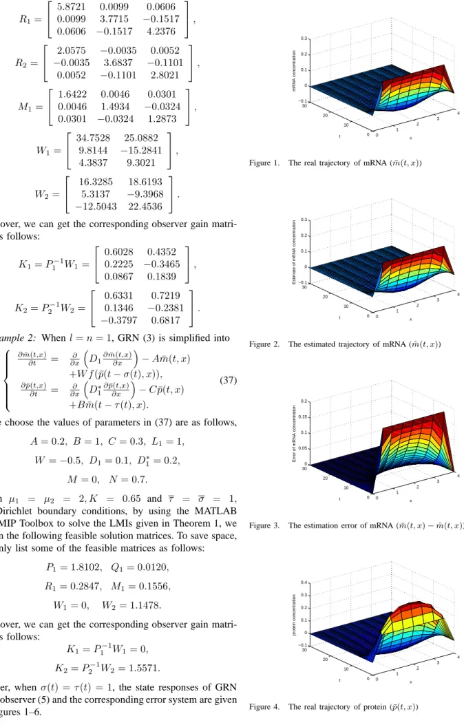
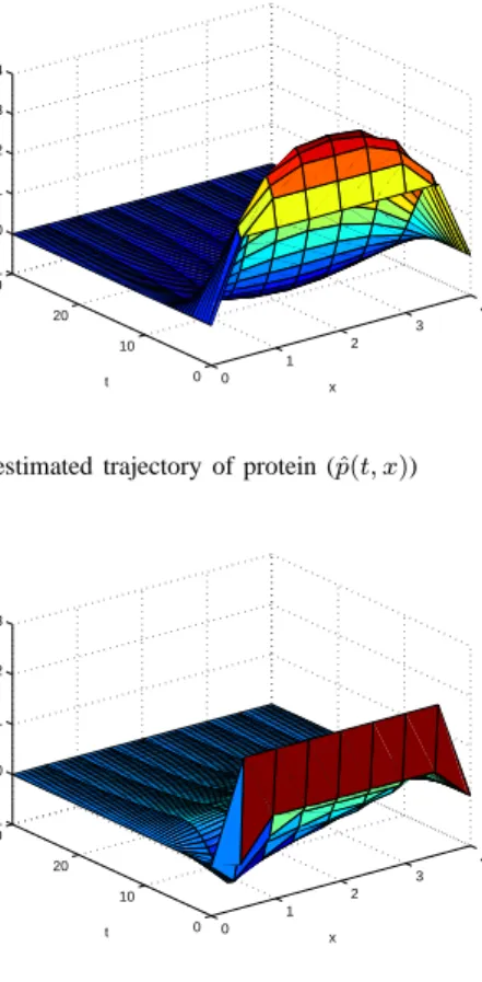
Further, when σ(t) =τ(t) = 1, the state responses of GRN (37), observer (5) and the corresponding error system are given in Figures 1–6. 0 1 2 3 4 0 10 20 30 −0.1 0 0.1 0.2 0.3 x t mRNA concentration
Figure 1. The real trajectory of mRNA (m¯(t, x))
0 1 2 3 4 0 10 20 30 −0.1 0 0.1 0.2 0.3 x t
Estimate of mRNA concentration
Figure 2. The estimated trajectory of mRNA (mˆ(t, x))
0 1 2 3 4 0 10 20 30 0 0.05 0.1 0.15 0.2 x t
Error of mRNA concentration
Figure 3. The estimation error of mRNA (m¯(t, x)−mˆ(t, x))
0 1 2 3 4 0 10 20 30 −0.1 0 0.1 0.2 0.3 0.4 x t protein concentration
0 1 2 3 4 0 10 20 30 −0.1 0 0.1 0.2 0.3 0.4 x t
Estimate of protein concentration
Figure 5. The estimated trajectory of protein (pˆ(t, x))
0 1 2 3 4 0 10 20 30 −0.1 0 0.1 0.2 0.3 x t
Error of protein concentration
Figure 6. The estimation error of protein (p¯(t, x)−pˆ(t, x))
V. CONCLUSIONS
In this paper, the state estimation problem for a class of GRNs with time-varying delays and reaction-diffusion terms are studied. An state observer is designed to estimate the gene states through available sensor measurements, and guarantee that the error system is asymptotically stable. By introducing new integral terms in a novel Lyapunov–Krasovskii functional and employing the so-called Wirtinger-based integral inequal-ity, Wirtinger’s inequalinequal-ity, Green’s second identity and, convex combination approach, RCC approach, a sufficient condition guaranteeing the existence of state observers is established in terms of LMIs. The concrete expression of the desired state observer has been presented in Theorem 1. Finally, two numerical examples are given to illustrate the effectiveness of the theoretical results.
REFERENCES
[1] H. De Jong, “Modeling and simulation of genetic regulatory systems: a literature review,” J. Comput. Biology, vol. 9, no. 1, pp. 67–103, 2002. [2] T. Akutsu, S. Miyano, S. Kuhara et al., “Identification of genetic networks from a small number of gene expression patterns under the Boolean network model,” in Pac. Symp. Biocomput., vol. 4. World Scientific Maui, Hawaii, 1999, pp. 17–28.
[3] D. Thieffry and R. Thomas, “Qualitative analysis of gene networks.” in
Pac. Symp. Biocomput., vol. 3, 1998, pp. 77–88.
[4] J. Cao and F. Ren, “Exponential stability of discrete-time genetic regulatory networks with delays,” IEEE Trans. Neural Networks, vol. 19, no. 3, pp. 520–523, 2008.
[5] Y. T. Wang, X. M. Zhou, and X. Zhang, “H∞ filtering for discrete-time genetic regulatory networks with random delay described by a Markovian chain,” Abstr. Appl. Anal., vol. 2014, pp. Article ID 257 971, 12 pages, 2014.
[6] T. T. Yu, J. Wang, and X. Zhang, “A less conservative stability criterion for delayed stochastic genetic regulatory networks,” Math. Probl. Eng., vol. 2014, pp. Article ID 768 483, 11 pages, 2014.
[7] X. Zhang, L. G. Wu, and S. C. Cui, “An improved integral to stabil-ity analysis of genetic regulatory networks with interval time-varying delays,” IEEE/ACM Trans. Comput. Biol. Bioinf., vol. 12, no. 2, pp. 398–409, 2015.
[8] X. Zhang, L. G. Wu, and J. H. Zou, “Globally asymptotic stability analysis for genetic regulatory networks with mixed delays: an M-matrix-based approach,” IEEE/ACM Trans. Comput. Biol. Bioinf., p. DOI:10.1109/TCBB.2015.2424432 (online), 2015.
[9] L. Wu, Z. Feng, and J. Lam, “Stability and synchronization of discrete-time neural networks with switching parameters and discrete-time-varying de-lays,” IEEE Trans. Neural Networks Learn. Syst., vol. 24, no. 12, pp. 1957–1972, 2013.
[10] Z. G. Wu, P. Shi, H. Y. Su, and J. Chu, “Sampled-data exponential synchronization of complex dynamical networks with time-varying coupling delay,” IEEE Trans. Neural Networks Learn. Syst., vol. 24, no. 8, pp. 1177–1187, 2013.
[11] J. D. Cao and Y. Wan, “Matrix measure strategies for stability and synchronization of inertial BAM neural network with time delays,”
Neural Networks, vol. 53, pp. 165–172, 2014.
[12] Z. G. Zeng and W. X. Zheng, “Multistability of neural networks with time-varying delays and concave-convex characteristics,” IEEE Trans.
Neural Networks Learn. Syst., vol. 23, no. 2, pp. 293–305, 2012.
[13] D. Yue and Q. L. Han, “Delay-dependent exponential stability of stochastic systems with time-varying delay, nonlinearity, and Markovian switching,” IEEE Trans. Autom. Control, vol. 50, no. 2, pp. 217–222, 2005.
[14] H. Li, H. Gao, and P. Shi, “New passivity analysis for neural networks with discrete and distributed delays,” IEEE Trans. Neural Networks, vol. 21, no. 11, pp. 1842–1847, 2010.
[15] P. Shi, X. Luan, and F. Liu, “H∞filtering for discrete-time systems with stochastic incomplete measurement and mixed delays,” IEEE Trans. Ind.
Electron., vol. 59, no. 6, pp. 2732–2739, 2012.
[16] T. T. Yu, X. Zhang, G. D. Zhang, and B. Niu, “Hopf bifurcation analysis for genetic regulatory networks with two delays,” Neurocomputing, vol. 164, pp. 190–200, 2015.
[17] G. D. Zhang, X. Lin, and X. Zhang, “Exponential stabilization of neutral-type neural networks with mixed interval time-varying delays by intermittent control: a CCL approach,” Circ. Syst. Signal Pr., vol. 33, pp. 371–391, 2014.
[18] R. Yang, H. Gao, and P. Shi, “Novel robust stability criteria for stochastic Hopfield neural networks with time delays,” IEEE Trans. Syst. Man
Cybern. Part B Cybern., vol. 39, no. 2, pp. 467–474, 2009.
[19] X. Zhang, A. H. Yu, and G. D. Zhang, “M-matrix-based delay-range-dependent global asymptotical stability criterion for genetic regulatory networks with time-varying delays,” Neurocomputing, vol. 113, pp. 8– 15, 2013.
[20] Y. T. Wang, A. H. Yu, and X. Zhang, “Robust stability of stochastic ge-netic regulatory networks with time-varying delays: a delay fractioning approach,” Neural Comput. Appl., vol. 23, no. 5, pp. 1217–1227, 2013. [21] D. Yue, E. Tian, and Q. L. Han, “A delay system method for designing event-triggered controllers of networked control systems,” IEEE Trans.
Autom. Control, vol. 58, no. 2, pp. 475–481, 2013.
[22] D. Yue, Y. Zhang, E. Tian, and C. Peng, “Delay-distribution-dependent exponential stability criteria for discrete-time recurrent neural networks with stochastic delay,” IEEE Trans. Neural Networks, vol. 19, no. 7, pp. 1299–1306, 2008.
[23] S. Busenberg and J. Mahaffy, “Interaction of spatial diffusion and delays in models of genetic control by repression,” J. Mol. Biol., vol. 22, no. 3, pp. 313–333, 1985.
[24] N. F. Britton, Reaction-Diffusion Equations and Their Applications to
Biology. New York: Academic Press, 1986.
[25] Y. Y. Han, X. Zhang, and Y. T. Wang, “Asymptotic stability criteria for genetic regulatory networks with time-varying delays and reaction– diffusion terms,” Circ. Syst. Signal Pr., vol. 34, pp. 3161–3690, 2015. [26] J. Zhou, S. Xu, and H. Shen, “Finite-time robust stochastic stability
of uncertain stochastic delayed reaction-diffusion genetic regulatory networks,” Neurocomputing, vol. 74, no. 17, pp. 2790–2796, 2011. [27] Q. Ma, G. D. Shi, S. Y. Xu, and Y. Zou, “Stability analysis for
delayed genetic regulatory networks with reaction–diffusion terms,”
Neural Comput. Appl., vol. 20, no. 4, pp. 507–516, 2011.
[28] Y. Y. Han and X. Zhang, “Stability analysis for delayed regulatory networks with reaction-diffusion terms (in Chinese),” J. Natur. Sci.
[29] B. Lv, J. L. Liang, and J. D. Cao, “Robust distributed state estimation for genetic regulatory networks with Markovian jumping parameters,”
Commun. Nonlinear Sci. Numer. Simul., vol. 16, no. 10, pp. 4060–4078,
2011.
[30] X. Lin, X. Zhang, and Y. T. Wang, “Robust passive filtering for neutral-type neural networks with time-varying discrete and unbounded distributed delays,” J. Franklin Inst., vol. 350, no. 5, pp. 966–989, 2013. [31] P. Shi, Y. Zhang, and R. K. Agarwal, “Stochastic finite-time state estimation for discrete time-delay neural networks with Markovian jumps,” Neurocomputing, vol. 151, pp. 168–174, 2015.
[32] Z. Wang, D. W. C. Ho, and X. Liu, “State estimation for delayed neural networks,” IEEE Trans. Neural Networks, vol. 21, no. 1, pp. 279–284, 2005.
[33] X. Zhang, X. Lin, and Y. T. Wang, “Robust fault detection filter design for a class of neutral-type neural networks with time-varying discrete and unbounded distributed delays,” Optim. Control Appl. Methods, vol. 34, pp. 590–607, 2012.
[34] K. Gu, “An integral inequality in the stability problem of time-delay systems,” in Proceedings of the 39th IEEE Conference on Decision and
Control, 2000, pp. 2805–2810.
[35] J. Sun, G. P. Liu, J. Chen, and D. Rees, “Improved delay-range-dependent stability criteria for linear systems with time-varying delays,”
Automatica, vol. 46, no. 2, pp. 466–470, 2010.
[36] A. Seuret and F. Gouaisbaut, “Wirtinger-based integral inequality: appli-cation to time-delay systems,” Automatica, vol. 49, no. 9, pp. 2860–2866, 2013.
[37] D. W. Kammler, A First Course in Fourier Analysis. Cambridge: Cambridge University Press, 2007.
[38] P. G. Park, J. W. Ko, and C. Jeong, “Reciprocally convex approach to stability of systems with time-varying delays,” Automatica, vol. 47, no. 1, pp. 235–238, 2011.