Classification and interpretation in quantitative structure-activity relationships

(1)

Bruce, Craig L. (2010) Classification and interpretation

in quantitative structure-activity relationships. PhD

thesis, University of Nottingham.

Access from the University of Nottingham repository: http://eprints.nottingham.ac.uk/11666/1/thesis-final.pdf Copyright and reuse:

The Nottingham ePrints service makes this work by researchers of the University of Nottingham available open access under the following conditions.

· Copyright and all moral rights to the version of the paper presented here belong to the individual author(s) and/or other copyright owners.

· To the extent reasonable and practicable the material made available in Nottingham ePrints has been checked for eligibility before being made available.

· Copies of full items can be used for personal research or study, educational, or not-for-profit purposes without prior permission or charge provided that the authors, title and full bibliographic details are credited, a hyperlink and/or URL is given for the original metadata page and the content is not changed in any way.

· Quotations or similar reproductions must be sufficiently acknowledged.

Please see our full end user licence at:

http://eprints.nottingham.ac.uk/end_user_agreement.pdf A note on versions:

The version presented here may differ from the published version or from the version of record. If you wish to cite this item you are advised to consult the publisher’s version. Please see the repository url above for details on accessing the published version and note that access may require a subscription.

(2)

Classification and Interpretation

in Quantitative Structure-Activity

Relationships

Craig L. Bruce, MChem.

Thesis submitted to the University of Nottingham

for the degree of Doctor of Philosophy

(3)

Abstract

A good QSAR model comprises several components. Predictive accuracy is paramount, but it is not the only important aspect. In addition, one should apply robust and appropriate statistical tests to the models to assess their signiﬁcance or the signiﬁcance of any apparent improvements. The real impact of a QSAR, however, perhaps lies in its chemical insight and interpretation, an aspect which is often overlooked.

This thesis covers three main topics: a comparison of contemporary classiﬁers, interpretability of random forests and usage of interpretable de-scriptors. The selection of data mining technique and descriptors entirely determine the available interpretation. Using interpretable approaches we have demonstrated their success on a variety of data sets.

By using robust multiple comparison statistics with eight data sets we demonstrate that a random forest has comparable predictive accuracies to the de facto standard, support vector machine. A random forest is inher-ently more interpretable than support vector machine, due to the underlying tree construction. We can extract some chemical insight from the random forest. However, with additional tools further insight would be available. A decision tree is easier to interpret than a random forest. Therefore, to obtain useful interpretation from a random forest we have employed a se-lection of tools. This includes alternative representations of the trees using SMILES and SMARTS. Using existing methods we can compare and clus-ter the trees in this representation. Descriptor analysis and importance can

(4)

be measured at the tree and forest level. Pathways in the trees can be compared and frequently occurring subgraphs identiﬁed. These tools have been built around the Weka machine learning workbench and are designed to allow further additions of new functionality.

The interpretability of a model is dependent on the model and the de-scriptors. They must describe something meaningful. To this end we have used the TMACC descriptors in the Solubility Challenge and literature data sets. We report how our retrospective analysis conﬁrms existing knowledge and how we identify novel C-domain inhibition of ACE.

In order to test our hypotheses we extended and developed existing soft-ware forming two applications. The Nottingham Cheminformatics Work-bench (NCW) will generate TMACC descriptors and allows the user to build and analyse models, including visualising the chemical interpretation. Forest Based Interpretation (FBI) provides various tools for interpretating a random forest model. Both applications are written in Java with full documentation and simple installations wizards are available for Windows, Linux and Mac.

(5)

Publications

1. Spowage, B. M.; Bruce, C. L.; Hirst, J. D. Interpretable Correla-tion Descriptors for Quantitative Structure-Activity RelaCorrela-tionships. J. Cheminf. 2009, 1:22.

2. Bruce, C. L.; Melville, J. L.; Pickett, S. D.; Hirst, J. D. Contempo-rary QSAR Classiﬁers Compared. J. Chem. Inf. Model. 2007, 47, 219-227.

(6)

Acknowledgements

Foremost thanks go to my supervisor, Jonathan Hirst. His guidance and patience have been paramount in completing this work. I am grateful to GlaxoSmithKline for funding and the many useful discussions, particularly my industrial supervisor, Stephen Pickett, and his colleagues Chris Lus-combe and Gavin Harper.

Thanks to both current and former members of the Hirst Group, espe-cially James Melville and Benjamin Bulheller. I thank Clare-Louise Evans and Haydn Williams for providing a productive, yet relaxed, oﬃce environ-ment.

I am grateful to the University of Nottingham for providing access to the High Performance Computing facility and the School of Chemistry for the Computational Chemistry facilities. In addition, thanks to the EPSRC for funding. I would like to acknowledge the academic licenses made avail-able from both OpenEye and ChemAxon, which have allowed this work to progress much further without the need to reinvent the wheel, so to speak. My current employer has encouraged and given me the opportunity to ﬁnish this work, even after I claimed it would be ﬁnished within a month. I thank Sandra McLaughlin and Andrew Grant for their extended patience given my huge underestimate of time required.

Finally, I am very grateful for the support from Michael McCusker and my family to see this work through to the end. It is to them I dedicate this completed thesis.

(7)

List of Figures

1.1 A sample graph depicting 12 nodes and 11 edges, representing propan-1-ol. . . 5 1.2 InChI and InChIKey for Lipitor. . . 8 1.3 Docking example. . . 14 1.4 A plot of the numbers of pairs of brooding storks and

new-born babies in West Germany from 1960 to 1985. . . 17 2.1 An example decision tree modelling Lipinski-like rules. . . . 26 2.2 Overview of bagging. . . 29 2.3 Overview of a random forest. . . 31 2.4 Separating hyperplane of the Support Vector Machine that

maximizes the margin between two sets of perfectly separable objects. . . 33 2.5 Aspirin. TMACC descriptors are based on topological

dis-tances. . . 44 2.6 A molecule from the ACE dataset in NCW, after the each

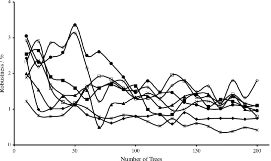
atom has been assigned an activity contribution by colour . 47 3.1 Robustness with increasing number of trees (on 2.5D

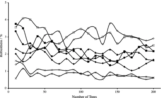
descrip-tors). . . 58 3.2 Robustness with increasing number of trees (on linear

(11)

3.3 Decision trees classifying activity of the ACE data set gen-erated by (a) the J48 algorithm with pruning and (b) the random tree algorithm without pruning. Descriptors deﬁni-tions are in Table 3.6 . . . 65 3.4 Percentage of model explained by unique descriptors for the

DHFR data set. . . 67 4.1 Summary of descriptor frequency across a forest using the

ACE data set . . . 83 4.2 Summary of descriptor frequency across tree 10 using the

ACE data set . . . 85 4.3 Weka tree visualiser with added navigation panel to view

trees in a forest . . . 86 4.4 A tree encoded as SMILES. Oxygen (O) is the root node. . . 87 4.5 A tree encoded as SMARTS. The wildcard atom type (A) is

the root node. . . 87 4.6 Summary of the majority vote for a forest built using the

ACE data set . . . 88 4.7 Molecule performance for a forest built using the ACE data set 89 5.1 ACE inhibitor features investigated. . . 97 5.2 TMACC interpretation of ACE inhibitors. A. Captopril. B.

Enalaprilat. C. Lisinopril. . . 98 5.3 Conserved ACE residues that interact with lisinopril. A)

tACE active site (green).172 _{B) The N-domain active site of}

sACE (purple).173

. . . 101 5.4 Comparison of the S1’ sub-site residues which bind the

ly-syl group of lisinopril. A) tACE (green)172 _{and B) the}

(12)

5.5 Predicted versus observed solubility for the training data (r2

= 0.79). . . 106 5.6 Predicted versus observed solubility for the cross-validated

data. . . 107 5.7 Predicted versus observed solubility for the 32 molecule set. 107 5.8 Predicted versus observed solubility for the 28 molecule set. 108 5.9 Predicted versus observed solubility for the 24 molecule set. 108 5.10 TMACC colour scheme . . . 108 5.11 A amiodarone, B diazoxide, C hydrochlorothiazide & D

pyrimethamine. . . 110 5.12 Aciprofloxacin,Bdanofloxacin,Cenrofloxacin &Dsparfloxacin.111

(13)

List of Tables

1.1 Examples of SMILES . . . 6

1.2 Examples of SMARTS . . . 9

2.1 A general confusion matrix . . . 35

2.2 Colour codes used in TMACC interpretation . . . 47

3.1 Summary of QSAR Data Sets . . . 56

3.2 Percentage of Correctly Classified Molecules for Different Clas-sifiers on 2.5D Descriptor Data Sets . . . 57

3.3 Mean percentage of correctly classiﬁed molecules for diﬀerent parameters of SVMs on 2.5D descriptor datasets. . . 60

3.4 Percentage of Correctly Classified Molecules for Different Clas-sifiers on Linear Fragment Descriptor Data Sets . . . 61

3.5 Mean percentage of correctly classified molecules for different parameters of SVMs on linear fragment descriptor datasets. 61 3.6 Descriptor definitions from the decision trees in Figure 3.3 . 66 4.1 Composition of GSK data set and distribution of classes . . 74

4.2 Default cost matrix. . . 76

4.3 Confusion matrix for the default random forest reporting the test set results. . . 79

4.4 Cost matrix for the cost sensitive random forest. . . 79

4.5 Confusion matrix for the cost sensitive random forest report-ing the test set results. . . 79

(14)

4.6 Confusion matrix for the oversampled random forest report-ing the test set results. . . 80 4.7 Cost matrix for the cost sensitive and oversampled random

forest. . . 81 4.8 Confusion matrix for the cost sensitive and oversampled

ran-dom forest reporting the test set results. . . 81 5.1 Frequency of activity of ACE inhibitor features as determined

by the TMACC interpretation. . . 100 5.2 Conserved ACE residues important for inhibitor interactions 102 5.3 Weka classiﬁers with multiple TMACC variants. . . 104 5.4 Number of attributes in diﬀerent variants of TMACC.

Num-ber of logS components refers to those included. . . 104 5.5 Errors for the cross-validation for the three techniques. . . . 104 5.6 Final two techniques with cutoﬀ of maximum topological

dis-tance . . . 105 5.7 GridSearch for C, γ and ǫ. . . 105 5.8 Test set compounds and their observed and predicted logS

values. . . 109 5.9 Results of solubility challenge, ranks against the other 99

entrants. . . 112 5.10 Results of solubility challenge, against performance markers.

The best and median results are also shown for comparison. 113 A.1 Solubility training set compounds . . . 143 A.2 Solubility test set compounds . . . 164

(15)

List of Abbreviations

ACE Angiotensin converting enzyme

AChE Acetyl-cholinesterase

API Application programming interface

BZR Benzodiazepine receptor

COX2 Cyclooxygenase-2

CPU Central processing unit

DHFR Dihydrofolate reductase

FBI Forest based interpretation

GPB Glycogen phosphorylase b

GPU Graphics processing unit

HPC High performance computing

HQSAR Hologram QSAR

InChI International Chemical Identiﬁer

LOO Leave one out

MAE Mean absolute error

(16)

NCW Nottingham cheminformatics workbench

PCR Principal component regression

PLS Partial least squares

QSAR Quantitative structure-activity relationship QSPR Quantitative structure-property relationship

RF Random forest

RMSE Root mean-squared error

SMARTS Smiles arbitrary target speciﬁcation

SMILES Simpliﬁed molecular input line entry speciﬁcation

SVM Support vector machine

SVR Support vector regression

THER Thermolysin

THR Thrombin

(17)

Chapter 1

Introduction

1.1

Industrial overview

There has been an increasing push within the pharmaceutical industry to accelerate the output of new drugs, as many of the blockbusters approach the end of their patents. The so called patent cliff is going to impact all big pharma at the cost of billions of USD per annum. In addition, there has been a long term drive to decrease the length of drug discovery. The time required to bring a drug to market takes up a large proportion of the patent lifespan. Improvements to efficiency and throughput can be applied to every step of the drug discovery process. The drug discovery process is a long chain of research and development. A new drug will take anything from 12-15 years to reach the market. This thesis covers techniques nor-mally used in lead generation and lead optimisation, both very early stage. Once a candidate compound has been validated using in silico methods, experimental data must support the hypothesis. Many filters and models exist to check for amongst other properties, bioavailability and toxicology. It is far better to drop a compound early rather than late. Each month in development accrues more expense which ultimately must be recouped by a successful drug, before itself making a profit. Candidate drugs enter animal and human trials at great cost. Each subsequent phase of testing

(18)

adds more rapidly increasing cost. In vitro studies are carried out first in test tubes before moving to in vivo studies in animals. The aim of these studies is to assess the response in living models. The dosage is also mea-sured. Human trials occur in several phases. Phase I is a small cohort of healthy volunteers. The candidate drug and placebo are measured to determine the effectiveness and safety in humans. Further dosage studies are conducted based on the animal models as they are only a guide. There can be substantially different responses between both. Phase II continues to measures safety and efficacy. Patients are included for the first time in Phase II, along with further volunteers, comprising a larger test population. Phase III trial employ a larger group to assess a wider variety of patients. The phase III trials typically continue while regulatory approved is applied for. A candidate drug can be withdrawn at any stage if the trials highlight undesirable toxicity, side effects or if the drug simply does not work. Each country requires a separate license making global distribution complicated, lengthy and expensive. In addition different clinical studies may be required to comply with local law. Clinical studies continue after launch to ensure no unforeseen issues arise as a wider population administer the drug. In some cases side effects may take years to manifest and hence clinical trials simply cannot check for these. A recent high profile case of side effects was Merck’s anti-inflammatory drug Vioxx. It led to an increased likelihood of heart attack and strokes. Merck voluntarily withdrew Vioxx after subse-quent studies confirmed the link. During the clinical trials process R&D will find a suitable synthesis for mass production and formulation for the chosen delivery method. Only a handful of candidate drugs ever reach the market. Previously pharmaceuticals thrived on multiple billon dollar drugs. Most of these reach patent expiry by 2015, leaving a huge gap in revenues. Few new drugs have reached the same profitability. In recent years it is now harder to register a drug and more expensive. The funding bodies

(19)

and insurance companies demand lower prices for patented drugs and when cheaper generics are an option they are often taken. Pharma has reacted to the changing marketplace by reshaping R&D and expanding into new ther-apeutic areas, e.g. personalised medicines. Companies will have more drugs targeted at smaller patient populations, while less proﬁtable, it removes the dependence on a few top earners. Biotechnology companies were hailed as the answer, many of which have now been bought by the pharma giants. Pharma themselves have continued to merge as well forming even bigger multinationals, which are now ready for restructuring and streamlining of costs. All eﬀorts are to produce more successful drugs for a fraction of the cost.

Patents are harder to obtain and are more frequently being challenged. The cost to bring a successful drug to market now is 800 million to 1.3 billion dollars. Late stage attrition is a strong contributor to this high cost. Once a candidate enters clinical trials the investment costs jump immediately. Even once oﬀ patent there used to be little competition from the generics. Now it is substantial. In addition, the various agencies across the globe drive for the cheapest price. The cost and duration of development is becoming increasingly prohibitive. All aspects of development can and should be reviewed to improve them. The whole ﬁeld of cheminformatics is essentially aimed at aiding the early stages of drug discovery. Unlike other disciplines in chemistry, cheminformatics is very closed aligned to the pharmaceutical and agrochemical industries.

1.2

Cheminformatics

While not the most well-known part of chemistry, it plays an important part in the delivery of in silico techniques. Cheminformatics was originally deﬁned by Brown in 1998.1 _{However, the subject has been in existence far}

(20)

describ-ing multiple substituents. Wiswesser line notation, the ﬁrst line notation to describe complex molecules was created in 1949.2 _{The American Chemical}

Society created the Journal of Chemical Documentation in 1961 which has now morphed into the Journal of Chemical Information and Modeling. It is no longer the only journal dedicated to cheminformatics.

Pivotal to cheminformatics’ development has been the growth and ca-pabilities of the computer, core to any cheminformatics technique. Chemin-formatics consists of several topics, which will be discussed brieﬂy: chemical data storage, substructure searching, similarity searching, clustering, dock-ing and QSAR to name a few. Most techniques are available as both 2D and 3D methods. 2D methods are primarily concerned with the topology of molecules. Conformers and stereochemistry are typically ignored un-like with 3D methods. 3D methods are typically more complex in order to model the extra data. Studies have found 2D methods can sometimes outperform 3D counterparts.3 _{This may sound counterintuitive but simpler}

methodologies can yield better results with less computational eﬀort.

1.2.1

Chemical data storage

The electronic storage of chemical data is crucial to computational tech-niques, yet even today there are many formats with advantages and disad-vantages for all. While it is simple to store a chemical structure as an image ﬁle, this encodes limited chemical information in a challenging format. Ma-chine readable ﬁles are necessary for tools to have access to the chemical information. A common storage method for chemical structures is using a molecular graph. A molecular graph uses graph theory from mathematics.4

A graph is a representation of nodes and edges. In a molecule the nodes represent atoms and edges the bonds. The atoms and bonds in a molecule are not homogeneous. There will be several types of both, which must be captured. A limitation of graph theory is it only details the topology of a

(21)

structure, e.g. what nodes are connected to which edges. There is no spatial arrangement information. A sample graph is depicted in Figure 1.1.

Figure 1.1: A sample graph depicting 12 nodes and 11 edges, representing propan-1-ol. The bond order is present on the edges.

Molecular graphs are the blueprints for the construction of SMILES (Simpliﬁed Molecular Input Line Entry Speciﬁcation).5 _{SMILES is a}

com-mon and popular format, partly due to its concise and human readable nature. Each molecule is represented by a single line of text corresponding to the atoms and bonds in the molecular graph. Atoms are represented by their atomic symbol. Due to the high frequency of hydrogen and sin-gle bonds they are implicit. Double and triple bonds are encoded as an equals, =, and hash ,#, symbol, respectively. Aromaticity is encoded by using lower case, c, for aromatic carbon and upper case, C, for aliphatic. Rings are denoted by numbering the opening and closing atoms of the ring with the same number. Multiple rings use sequentially increasing numbers to identify them. Branching chains are handled by encasing all branched atoms in parentheses. Table 1.1 depicts several sample SMILES.

A given molecule can have multiple, yet valid, SMILES strings. Start-ing at diﬀerent atoms will result in a diﬀerent path through the molecule. However, the molecule is identical. This can lead to duplicate SMILES in

(22)

SMILES Name Depiction c1ccccc1 Benzene CS(=O)(=O)c1ccc(cc1)C2-=C(C(=O)OC2)c3ccccc3 Vioxx CC(C)c1c(C(=O)- Nc2ccccc2)c(c(c3ccc(F)- cc3)n1CC[C@@H]- 4C[C@@H](O)CC(=O)-O4)c5ccccc5 Lipitor CN1CC[C@]- 23[C@H]4Oc5c3c- (C[C@@H]1[C@@H]-2C=C[C@@H]4O)ccc5O Morphine

(23)

a database, which is highly undesirable. To provide a unique representa-tion the SMILES must be canonicalised. All variarepresenta-tions of a single molecule should resolve to the same canonical SMILES.6 _{There are now various}

algo-rithms for canonicalisation. Used consistently they provide unique SMILES. Although the molecular graph does not contain any spatial data, SMILES can encode limited stereochemical information, such as chiral centres and cis-trans isomers. As SMILES do not contain spatial information they are not suitable storage for 3D methods. In docking the ligand and protein, 3D information is paramount to the technique. 3D information is stored us-ing connection tables which contain Cartesian coordinates. Many formats use this method such asPDB(Protein Data Bank) andSDF(Structure-Data File). Typically the xyz coordinates of each atom are detailed along with each bond connections by atom ID.

Competing formats have arisen over time. One such example is the InChI (IUPAC International Chemical Identiﬁer).7 _{Designed by IUPAC}

with an aim to be freely available, computable by anyone and have a human readable quality, they encode more information than SMILES and address some of its weaknesses, e.g. the need for canonicalisation for uniqueness. The algorithm is a three step process: normalisation, canonicalisation and serialisation. Redundant information is removed, atoms are uniquely iden-tified and the output written as a string. Additionally, an InChIKey (or hash) can be generated, which is not human readable and is a fixed 25 character string. It was introduced for practical reasons around web based searches as the full InChI can be overly verbose. The main InChI is com-posed of up to six layers of information comprising the core layer, charge, stereochemistry, isotopic, fixed hydrogens and reconnected layer. The core layer comprises three sublayers: chemical formula, connectivity and hydro-gens. Only the chemical formula sublayer is required for a valid InChI. Each layer, and sublayer, is delimited by a slash,/. The InChiKey is based

(24)

on a hash algorithm. The first 14 characters determine the connectivity, while all additional information is encoded in the eight characters after a hyphen. The final two characters encode the InChI version and a checksum. The InChI and InChIKey for Lipitor is shown in Figure 1.2. While many vendors have added InChI support to their applications they have yet to receive widespread use over SMILES. SMILES have been the dominant 2D data format for many years. An OpenSMILES specification is being drawn up to address the original shortcomings.8

InChI=1S/C33H35FN2O5/c1-21(2)31-30(33(41)35-25-11-7- 4-8-12-25)29(22-9-5-3-6-10-22)32(23-13-15-24(34)16-14-23)- 36(31)18-17-26(37)19-27(38)20-28(39)40/h3-16,21,26-27,37-38H,17-20H2,1-2H3,(H,35,41)(H,39,40)/t26-,27-/m1/s1 OUCSEDFVYPBLLF-KAYWLYCHSA-N

Figure 1.2: InChI and InChIKey for Lipitor.

Complementing SMILES are SMARTS, SMiles ARbitrary Target Speci-ﬁcation,9_{a query language to search compound collections. Similar notation}

to SMILES is used, such as bond notation. Additional syntax is required to capture regular expression patterns. Carbon can be matched with its atomic number,[#6], aliphatic or aromatic carbon,[C,c]or the atom wildcard,*. Connectivity can be specified using[CX4], where the carbon must have four bonds. Carboxylic acid is represented as[CX3](=O)[OX2H1], a carbon with three bonds, connected via a branched double bond to an oxygen and to an-other oxygen. The second oxygen has two bonds, one of which connects to a single hydrogen. Logical operators of and,;, and or,,, are available to form patterns such as a primary amide: [N;H3;+][C;X4], charge represented by + or -. SMARTS therefore represent a powerful yet flexible query lan-guage in which to encode chemical queries. SMARTS are routinely used in substructure searching, fragment based approaches, scaffold building and combinational chemistry. SMARTS are more complicated than SMILES, but encode more information, and hence are typically more verbose. Table 1.2 depicts various SMARTS examples.

(25)

SMARTS Name Depiction

[CX4] Alkyl carbon

[CX3]=[OX1] Carbonyl group

[$([CX3]=[OX1]),-$([CX3+]-[OX1-])]

Carbonyl group, either resonance form

[#6][F,Cl,Br,I] Carbon attached

to a halide

(26)

The plethora of chemical formats now available can pose a barrier, es-pecially as commercial vendors typically introduce their own as well (e.g.

oebfrom OpenEye and moefrom the Computing Computing Group). Var-ious conversion tools exist. The best known is open Babel. However, some formats are less formalised than others leading to incorrect conversions.

1.2.2

Substructure searching

Often a database of compounds needs to be searched. Using either SMILES or SMARTS, depending how precise the query is, this can be quickly achieved. Many search methods already exist within graph theory. Substructure searching is essentially comparing two graphs to see if the query graph is rep-resented in the other. This is known as subgraph isomorphism. Established subgraph searching methods perform poorly in large chemical databases, as they are exhaustive searches. A two step process is now used, in which the first step removes the majority of query compounds, leaving a minority for the exhaustive subgraph matching. A binary representation of the molecule is used, as binary calculations can be performed very efficiently. A chemical dictionary is used to represent the structural features present in a molecule. If a given feature is present a 1 is entered to the bitstring, otherwise a 0. In order for the molecule to pass onto subgraph matching the bitstrings must match. Therefore, as soon as differences appear in the bitstring the compound is discarded, as it will not match. Using the reduced database the subgraph isomorphism search is executed. It belongs to a class of prob-lems known as NP-complete. NP-complete problems are characterised by an exponential relationship between the amount of time required and the size of the problem. This is because they are an exhaustive or brute-force approach. Therefore, it is prudent to avoid them when possible.

(27)

1.2.3

Similarity searching

Substructure searching is useful but often we do not have a complete query or want to ﬁnd an alternative structure. Similarity searching is based on the similar property principle that states similar structure often leads to similar properties.10 _{Therefore, the ability to ﬁnd similar compounds is of}

interest. SMARTS could be constructed to become increasingly fuzzy, but to capture all possibilities is non-trivial. Sometimes only a small fragment of interest is known and one needs to ﬁnd similar compounds. When dealing with 3D structure, similar compounds are more relevant than substructure matches, as the conformation becomes increasingly important. 2D similarity is computed by using the bitstrings used for substructure searching.

Molecular ﬁngerprints are the bitstring representation of molecules us-ing binary values.11 _{Two ﬂavours exist, the use of a fragment dictionary}

and hashed fingerprints. Fragment dictionaries use a predetermined list of structural features to represent each bit. Thus, you can map back to the structural element from the bitstring. This can make interpretation more accessible. Using hashed methods a predefined dictionary is not required, an advantage as any fragment present will be encoded. Using a dictionary you control what fragments are available and therefore can bias the fingerprint. Hashed fingerprints are unique per dataset and not readily interpretable in the same manner as a dictionary method. Fingerprints are now a popu-lar basis for descriptors, even though their conception was never intended for this. 2D fingerprints were originally developed to accelerate substruc-ture searching algorithm performance.11 _{There is no intrinsic reason why}

they should perform well as descriptors. The good performance is likely because the molecule’s properties and biological activity are dependent on the features encoded by the ﬁngerprint.

A similarity coeﬃcient is required to compare the bitstring representa-tion of molecules. There are numerous similarity coeﬃcients available. One

(28)

of the most common is the Tanimoto (or Jaccard) coeﬃcient. It can be expressed as SAB,

SAB =

c

a+b₋c (1.1)

where a are the bits sets in that target structure, b the bits set in the database structure andcthe bits set common in both structures. The result is a value between zero and one, where zero is no similarity and one an exact match. Results can then be sorted or restricted based on this measure. In addition to the other coeﬃcients used in other disciplines similarity can also be calculated via compression.12

1.2.4

Clustering

Cluster analysis is useful for large data sets. Clustering aims to group sim-ilar compounds together. The simsim-ilarity of the group members could be activity, therapeutic target or mode of action depending on the descriptors available. Typically clusters are made based on distance measures between other members of the data set. Most methods are also non-overlapping; each member belongs to only one cluster. Two types of methods are com-mon: hierarchical and non-hierarchical. Hierarchical methods compare all members to each other. They create clusters of decreasing size, with each smaller cluster being a subset of the larger cluster. They are much like a decision tree in this respect, especially as a dendrogram is used for visual-isation. Unlike a decision tree the clusters start as single compounds and grow as members are reorganised from the bottom up. Ward’s method is based on distance from one member to all others with the aim of minimising variance, without a dendrogram.13_{The user often needs to pick the number}

of required clusters. This can be done manually retrospectively or cluster level selection methods now exist to determine a balance of cluster num-ber and tightness of the clusters. The Jaccard statistic is used to compare

(29)

cluster groupings. Non-hierarchical clustering is normally done using the Jarvis-Patrick method.14 _{The data set is only read once in this method.}

The ﬁrst compound forms the ﬁrst cluster. The second joins if a criterion is met otherwise it forms a new cluster. Hierarchical clustering allows multiple comparisons of all data points. A drawback of this method is the presence of singletons, clusters with one member. By altering the rules for joining or making a new cluster the number of singletons can be reduced.

1.2.5

Docking

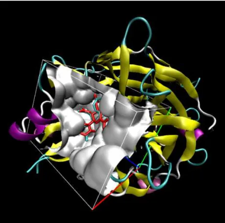
Docking is typically used to model how a given set of ligands would interact with a protein. Many drugs have protein targets and understanding their interaction is key to designing a potent compound. This is a 3D experiment where the conformation of the ligand in the protein pocket, or binding site, is explored to find the most energetically favourable pose. Protein structures are not fixed. The presence of a ligand will by design alter the conformation of the protein. This may be key in allowing the ligand to bind. Accurate protein behaviour is important to modelling realistic binding. The solvent of the system should also be taken into account as gas-phase simulations are not representative of a biological system. Ideally an experiment will start with a known crystal structure to which a theoretical ligand will be bound. A sample docking of the actual structure and best pose is shown in Figure 1.3. Initial methods assumed rigid-body structures, which is not ideal. More modern techniques allow flexible docking of both protein and ligand giving a more accurate representation. Flexible docking is far more computationally expensive, especially when a large set of ligands is used. Docking is a challenging technique as there are many hurdles. The crystal structure of the protein is the interpretation of the original crystallographer. Protein structures devised from homology modelling are even more subjective. If the protein structure is incorrect expecting reasonable binding energies is

(30)

unrealistic. The binding energy represents the non-covalent interactions between the ligand and protein. A force ﬁeld approach would use van der Waals and electrostatic interactions between all atoms of both molecules to predict the binding energy.

Figure 1.3: Docking example. Only the atoms in the box are used for calculation purposes. The red molecule is the crystal structure and blue the best docked pose.

1.3

Quantitative Structure-Activity

Relation-ships

QSAR (Quantitative Structure-Activity Relationship) is the focus of this thesis. It was ﬁrst used in the seminal work by Hansch15,16

. Hansch devised an equation relating descriptors of electronic properties and hydrophobicity to biological activity.

(31)

log µ 1 C ¶ =k1logP +k2σ+k3 (1.2)

where C is the concentration of compound needed to produce a standard response in a given time. logP is the octanol-water partition coeﬃcient and σ is the Hammett substitution parameter. Hansch also proposed that activity was parabolically dependent on logP:

log µ 1 C ¶ =₋k1(logP) 2 +k2(logP) +k3σ+k4 (1.3)

The reasoning for parabolic dependence on logP was the compound hydrophobicity should not be so low as not to cross the cell membrane, or so high that once in the membrane it remains in situ. Electronic parameters are important in determining activity. The Hammett parameters come from Equations 1.4 and 1.5. The equations quantify related compound reaction rates and positions of equilibrium.

log µ k k0 ¶ =ρσ (1.4) log µ K K0 ¶ =ρσ (1.5)

wherek is the rate and K is the equilibrium constant for a particular sub-stituent relative to a reference compound (typically hydrogen, corresponds tok0 andK0). Hammett used the hydrolysis of benzoate esters to measure

reaction rates and ionisation constants of substituted benzoic acids for equi-libriums. The parameterσ is determined by the nature of the substituent and whether is is meta or para to a group on the aromatic ring. The reac-tion constant ρ is ﬁxed for a particular process. Since Hammett’s original work17 _{there have been various advances.}18

(32)

descrip-tors considered. There are three components to a QSAR model: the data, how one represents the data and the statistical technique chosen to find a relationship between them. All three affect the overall model produced. All models should be thoroughly validated to ensure they are predictive. While the classic QSAR dataset is small (about 30 compounds) it is now widely acknowledged that this can be too small.19 _{One cannot expect to find a}

relationship from so few datapoints. 60 compounds has been suggested as the minimum size for a dataset.20

Tens of thousands of descriptors can be readily generated in silico. On ﬁrst inspection one may think more descriptors means an improved model. However, in reality the noise and cross-correlation of the descriptors can confuse the learning algorithm. Better performance can be achieved with a smaller number of descriptors. Indeed techniques exist to perform attribute selection before building the primary model as increased descriptors can im-pact the model generation signiﬁcantly. Some machine learning techniques inherently perform this step.

Popular algorithms for QSAR are decision trees, neural networks, genetic algorithms, support vector machine (SVM), partial least squares (PLS) and ensemble methods, e.g. random forests. Further details of these algorithms is detailed in Chapter 2. The literature is full of examples of all these algorithms on various targets and various comparisons. Although no modi-ﬁcation to the algorithm is required, many algorithms have had some mod-iﬁcation, for example making neural networks more interpretable21,22_,

con-structing chemical kernels23,24_{for SVM and multiple variations on PLS}25,26_.

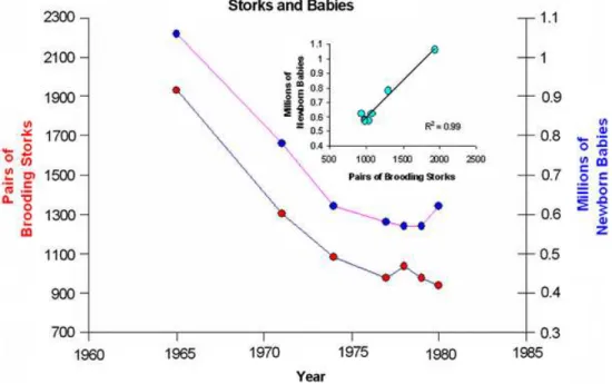
Recently, several articles have questioned the usefulness of QSAR, for example, when excellent models in terms of q2 _{(deﬁned in Chapter 2) can}

be found between number of brooding storks and newborn babies (Figure. 1.4).27 _{How can we expect QSAR to ﬁnd meaningful chemical relationships}

(33)

but ensuring they are used correctly. Larger data sets and interpretable de-scriptors, are just two areas for improvement. The use of multiple statistics to measure the model, not justq2 _{is important, as a single statistic can be}

misleading. Rigorous statistics should be used to compare techniques. The community must push best practices to enable further advances in the ﬁeld.

Figure 1.4: A plot of the numbers of pairs of brooding storks and new-born babies in West Germany from 1960 to 1985. Representation of the data as a correlation plot (Inset). With permission from Springer Science+Business Media: Journal of Computer-Aided Molecular Design, QSAR: dead or alive?, 22, 2008, 82, Arthur M. Doweyko, Figure 1,

c

°Springer Science+Business Media.

QSAR is analogous to QSPR (Quantitative structure-property predic-tion). We show a QSPR example later when we predict solubility as part of the solubility challenge organised by the Journal of Chemical Information and Modeling. Solubility is an important property of a drug, but hard to estimate both experimentally and computationally. It is the ability of a sub-stance to dissolve in a solvent. Drugs need to be water soluble in order to be orally bioavailable, which is the preferred method of administration. Drugs which are not water soluble cannot be tested in biological assays, have poor pharmacological proﬁles and tend to precipitate in storage.28 _{Solubility is}

(34)

which must be reduced. Current computational models for solubility can have an error of an order of magnitude. This is compounded by a lack of reliable and reproducible experiment data.

Drug discovery is a multi-variate problem. For example, while one can create a model for activity, it is useless if the compounds do not have a suitable solubility. Even once these are overcome, other obstacles will likely challenge the path to successful registration. Many factors contribute to sol-ubility, making prediction challenging. These include lipophilicity, number of hydrogen bonds formed in solvent, the ability to form intramolecular hy-drogen bonds, the ionisation states of functional groups and the properties in crystal form.29

The field, in general, has seen numerous advances over the last few decades especially in QSAR, mainly from 2D all the way to 6D. Admittedly 2D and 3D are the most commonly used. 2D QSAR uses descriptors based on the 2D topology of the molecule. This can include 3D values such as vol-ume or surface area. However, these values are typically calculated without multiple conformers and possibly without 3D coordinates if SMILES are the input data format. 2D QSAR uses machine learning algorithms to find a re-lationship between the descriptors and activity. 3D QSAR has two popular flavours, Comparative Molecular Similarity Indices Analysis30 _(CoMSIA)

and Comparative Molecular Field Analysis (CoMFA).31 _{CoMFA attempts}

to find a correlation between activity and 3D shape, electrostatics and hy-drogen bonding. The biologically active conformation for each molecule is required. Each conformation has molecular fields generated. The fields are calculated with the molecule in a lattice, thus allowing comparison to all other molecules. Typically electrostatic and steric probes are used at each defined point within the lattice. PLS is used to analyse the data generated from the lattice. The coefficients obtained from PLS allow 3D contour plots to be generated on the lattice. The contours indicate regions where charged

(35)

groups or steric bulk can aﬀect activity (both in a positive and negative fashion). CoMSIA was developed after CoMFA and addresses some of its drawbacks.

The fourth “dimension” in the paradigm is sampling and includes the sampling of conformation, alignment, pharmacophore sites and entropy.32

The composite information coming from each of these sampled property sets is embedded in the resulting QSAR model. Most of the other n D-QSAR methods consider each of these properties, which are sampled as individual dimensions in their QSAR studies. Hence one would get a 5D QSAR33_{method if conformational sampling is included, and a 6D QSAR}34

approach if both conformational and alignment samplings are considered.

1.4

Pragmatic programming

Computational tools have advanced both commercially and from open source projects. A range of programs are now available to assist from various com-mercial suppliers. One of the most useful features is access to an application programming interface (API), as invariably one always wants to do some-thing slightly outside the scope of a program. Weka20_{is a machine learning}

workbench; Marvin35_{allows for the sketching and visualisation of molecules.}

Both programs are written in Java enabling them to work cross-platform. NCW and FBI, the two packages which result from this thesis were possible through the availability of the API for Weka and Marvin. Without the API a huge amount of additional coding would of been required. In addition, these tools have already been validated by the community. NCW and FBI are discussed in Chapters 5 and 4 in more detail.

Weka is an open source application that allows us to modify the source if necessary or extend the API. Marvin is not open source but the API is mature and was capable of accomplishing our tasks. The modern day computational chemist or cheminformatician requires a strong grounding in

(36)

computer science to beneﬁt from all the tools available. Indeed, chemin-formatics has seen a explosion of software packages and web services. This is only set to rise as Research Councils encourage open source publication of work they have funded. Some programs have gone on to form commer-cial spin outs from universities. Some programs funded over the long term have become very successful, Weka is an example, ﬁrst introduced in 1993. From the cheminformatics world KNIME36 _{is becoming increasingly}

popu-lar as an open source alternative to Pipeline Pilot.37_{It optionally runs Weka}

and use commercial plug-ins from Schr¨odinger38 _{who part fund its ongoing}

development.

Producing programs as a result of a research projects can be problem-atic, as once complete they often are left unmaintained. Many such projects were seen during this research. This was one reason for the introduction of NCW to encapsulate the in-house code built up over the years into a single maintainable package. The pragmatic programming approach also aids this.39 _{There are three principles to follow: version control, testing}

and continuous integration. First, a collection of source files is no good to anyone; documentation, compilation instructions and any dependencies are required. Version control is a repository of source code (or any file) which keeps a record of all the changes to a project. The repository’s ability to compare and revert to older revisions is very useful, as well as the simple fact that all the required files are in one place. Popular version control programs are subversion40,41_{and git}42_{; both follow a different methodology.}

Second, how can one know what code is supposed to do? Documentation is normally thin, rarely extensive. Unit tests provide the programmer with some confidence in the code, but third parties can view unit tests as sam-ple code usage. Unit tests enable code verification and validation. In Java the unit test is written in a separate source file and tests public methods within the class. Tests in Java are known as JUnit tests. Third,

(37)

contin-uous integration allows repetitive deployment tasks to be automated and performed by a schedule and on demand. CruiseControl is a popular open source choice.43 _{Once conﬁgured it detects any change to one’s source}

con-trol repository then checks out the latest code, builds it, running any tests as well. Not only does this save the developer time performing extra steps (which often would not be carried out), it can highlight errors very quickly; from test failures to missing dependencies on the build machine. Compila-tion is always simple on the developer’s machine. The clean build machine is used to highlight hidden dependences. Both NCW and FBI follow these three pillars of software development. In addition, CruiseControl can auto-mate packaged installers using IzPack. IzPack is a Java based GUI wizard installer.44_{Once CruiseControl has compiled the basic source IzPack creates}

an installer. CruiseControl also packages it ready for easy deployment on Windows, Mac and Linux. After each source change everything is deleted and built from scratch, ideally ending with one’s deployment ﬁles ready to go, or an email highlighting the error and modiﬁcation to the source since the last successful build. This is far quicker than a developer could do, saving time and allowing others to access the compiled code easily.

1.5

High Performance Computing

To generate large numbers of QSAR models more than a single workstation is required. For a combination of reasons including data set sizes and al-gorithm complexity, model generation time is increasing. The use of High Performance Computing (HPC) is prevalent within science already. Within Chemistry, molecular dynamics andab initio calculations are common tasks for HPC. HPC clusters can readily generate large numbers of QSAR mod-els. To take advantage of computational advances algorithms are being written with parallel coding. The use of parallel programming standards can reduce computation on multi-cores computers which are the de facto

(38)

standard now. Previously, HPC has utilised parallel computation across physical computers. This requires rewriting your software and having a cluster with suitable parallel connectivity. The latest parallel advances re-late to the same hardware, not clusters. However, merging both forms of parallelism is possible and advantageous. Universities and industry alike both have HPC facilities available for researchers. HPC is dominated by the Linux operating system. Most HPC codes were never written for Win-dows. Scientific computing is firmly a task for Linux. Queuing systems are available for HPC as many users will want access to the compute re-source. Sun Grid Engine is a well known example. It enables users to submit jobs to the queue and it will process them according to priority, hardware requirements and resources available. Traditional HPC is carried out on large, purpose built, homogeneous clusters. This typically represents a large investment from the institution, but has defined outcomes (in terms of compute ability). More recently a different model, Grid computing, has become popular. Grid computing varies from HPC as it does not rely on dedicated resources. The key concept of Grid computing is a dynamic pool of resource that is constantly changing for various reasons. With this set up queues are handled differently and rules are in place for when non dedi-cated resource is being used. The appeal of Grid computing is the ease at which the pool size can grow by utilising existing hardware. The standard workstation today is more powerful than dedicated HPC cluster nodes only a few years ago. However, after 5pm these workstations sit idle, wasting electricity and CPU cycles. Grid computing enables you to tap into this resource. From a cost perspective this is an attractive route to increase total compute resources. Condor is a popular program to manage a grid clusters. Grids are not bound by geographic location, unlike HPC which tend to represent a physical set of hardware. BOINC, another grid sched-uler, runs many public research projects on volunteer computers across the

(39)

world. Using Condor one can achieve similar global pools.

Computational hardware and software develop at astonishing rates, and continue to do so. In order to exploit these advances our scientiﬁc software must make use of these developments. There is a cost with parallel or sim-ilarly advanced coding paradigms - they are increasingly complex to write. One requires a ﬁrm understanding of the base language before attempting to parallelise code. In this respect one needs to be a more accomplished programmer to fully leverage the resources available. Although challenging, the return is impressive. GPUs (Graphical Processing Units), another form of parallelism on GPUs opposed to CPUs can achieve speed improvements of one hundred fold.

1.6

Summary

QSAR needs to remain in favour with cheminformaticians. This can be achieved by using appropriate statistics that correctly represent the data and exploiting the chemical insight within the model. Suitable statistics is a matter of good practice and not using any one measure to determine how useful a model is. The presence of readily available interpretation would be desired by any modeller. Robust statistics and reliable interpretation will lead to greater conﬁdence in models. This is not to say models are perfect predictions, they are not. However, if the one has chemical insight available and a measure of conﬁdence then an informed decision can be made based on the data.

In the following chapters we will test various hypotheses. We will assess, by means of multiple comparison statistics, if random forests oﬀer competi-tive prediccompeti-tive ability to support vector machine using multiple data sets. In order to assess multiple classiﬁers, data sets and parameters in a timely fash-ion high performance computing schedulers will be employed. It is already known that random forests are interpretable. However, the practicality of

(40)

accessing this interpretation has received less attention. The volume of 100 trees makes manual interpretation unattractive. We will investigate tools to assist in dealing with this number of trees. The TMACC descriptors have demonstrated predictive ability. They are interpretable but this has not been validated in detail. We will retrospectively test data sets to see if the TMACC interpretation matches that reported in the literature.

(41)

Chapter 2

Methods

2.1

Learning classifiers

While QSAR has a relatively long history for a computational method, mod-ern QSAR borrows directly from the machine learning techniques of data mining. Neural networks and SVM are two such examples. The goals of QSAR and data mining do not overlap entirely. While both are concerned with generating a model to explain an unknown relationship, only QSAR has the secondary goal of model interpretation. The inner workings of a model based on chemical insight are invaluable, more so than mining credit card spending habits, for example. The ability to interpret is speciﬁc to the model. Some are straightforward; others are not. This would not be a primary concern when a new technique is designed. However, for use in drug discovery it is tremendously useful. There has been lots of work inter-preting learning classiﬁers, e.g. neural networks, that were not interpretable originally.21 _{It is arguable that interpretation is more important than}

im-provements in prediction accuracy. Next, the various learning classiﬁers used in this thesis will be discussed.

(42)

2.1.1

Decision tree

The decision tree,45 _{also known as recursive partitioning, is essentially a}

collection of decision stumps. Each stump is a split of the instances available according to the attribute with the greatest purity. The purity for a given attribute is the fraction of correctly classified instances. In the full tree each split results in two subsets of instances. Both of these are now split again on the purest attribute. This continues recursively, until a stopping criterion is met, typically a minimum number of instances. The splits are known as branches, while the collection of classified instances is a leaf. The tree is a collection of both. Afterwards a pruning algorithm is applied, which reduces the tree to the core components. The result is typically smaller than the original tree, which helps to reduce overfitting. Duplicate branches and/or leaves can be removed during this process and the tree can have a more lop-sided appearance. A decision tree modelling Lipinski-like rules46_{can be}

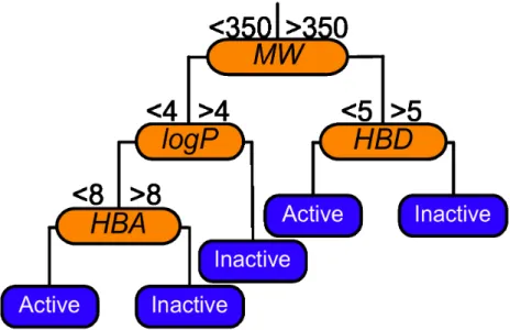
seen in Figure 2.1.

Figure 2.1: An example decision tree modelling Lipinski-like rules. Molecu-lar weight (MW) should not exceed 350. The octanol-water partition coef-ficient (logP) should be below four. Hydrogen bond donors (HBD) should not exceed five. Hydrogen bond acceptors (HBA) should not exceed eight. Note the classifications of active or inactive refer to meeting Lipinski rules, not molecular activity.

(43)

Once a tree is built it can be used on external data to produce a classiﬁ-cation and a set of rules determined by the path travelled through the tree. More than two splits per branch is possible. In Weka20 _{only two splits per}

branch are allowed. However, multi-classiﬁcation problems can be solved. Due to the construction of the tree, the time to generate it can be predicted in advance.

2.1.2

Ensemble methods

To improve the performance of single classiﬁers, ensemble or meta ap-proaches have been developed. Of note are bagging, see section 2.1.3, boost-ing, see section 2.1.4 and stackboost-ing, see section 2.1.5. The premise behind the technique is that 100 experts will, on average, provide a better answer than a single expert. If there are disagreements the majority and other methods can be used to determine the overall ensemble answer. There has been much research into how these techniques work.47–49 _{Some results have}

proved diﬃcult to explain, for example adding random variance to bagging will improve the performance. Boosting has been the subject of extensive analysis and not until its close relation to additive learning became appar-ent was it understood.50 _{Bagging and boosting are concerned with using}

the same classifiers for the whole ensemble, whereas stacking can mix any number of different classifiers together. Both approaches work well, as one would expect by repeating the same technique multiple times or combining multiple results together. It should be noted that each replica is unique in some fashion. In bagging different data is used for each classifier. Stacking is also appealing, as there is no single silver bullet for the optimal classifier. It is widely accepted that one must try a selection of classifiers. However, as a rule of thumb certain techniques such as SVM and random forest generally perform well. There is always the exception, as demonstrated in Chapter 3, where a single decision tree outperforms several more advanced techniques,

(44)

including SVM and random forest.

The prediction error of an ensemble is related to the error of the indi-vidual classiﬁers:

M SEEnsemble =

1

NM SE (2.1)

where M SE is the average mean squared error, M SE of individual mem-bers and N is the number of members in the ensemble. As the number of members increases the theoretical error is smaller than that of a single member.51 _Increasing_N _{indeﬁnitely will not yield constantly improving}

ac-curacy; the improvement may become very small. In addition increasing the ensemble size will increase compute time, which may be undesirable. The error of an individual member can be expressed in bias and variance:

M SE =V ariance(ˆθ) +Bias2(ˆθ) (2.2) where ˆθ is a estimator of the quantity θ. Model bias decreases as model variance increases. This would seem reasonable. As the model becomes more complex, the bias towards any single instance will decrease. There is a trade-off between these two functions. Ideally, both should be low. However, as one adds data to reduce the bias, the variance will increase. The ideal model will balance both functions, but still maintain good predictive power and avoid overfitting. Ensembles achieve predictive improvement by reducing the variance in their members and leaving the bias unaltered. By taking advantage of the bias and variance trade-off the ensemble can obtain a lower prediction error than any single member.

2.1.3

Bagging

While trees oﬀer relative straightforward interpretation, they are less ac-curate than state-of-the-art techniques, such as SVM. Ensemble techniques

(45)

such as bagging offer improvements over a single classifier. Bagging is a simple, yet effective approach. One creates n bags of the original data set by sampling with replacement, thus allowing the same instance into the same bag. With each of the n unique bags, one builds a model using any chosen classifier, e.g. a decision tree. For each instance, there aren predic-tions and a majority vote decides the overall classification. One drawback of meta techniques is the increase in model generation time. This exam-ple takesn times longer than a single tree, but will build a more predictive model. This is an example of Occam’s razor,52_{where one must balance}

per-formance with accuracy. Bagging lends itself to parallelism via the many methods now available in computer science, such as threading and grid computing. Bagging is depicted in Figure 2.2.

Figure 2.2: Overview of bagging. The training data set is used to generate ten re-sampled data sets known as bags. Each will be unique. A classifier is built for each bag. Different data ensures different models. A majority vote across all classifiers determines the ensemble prediction. Ten bags are for depiction purposes. Breiman used 50 in his original study, but found a lower number, could be optimal.53

2.1.4

Boosting

Boosting is a technique developed after bagging. It is widely reported to outperform bagging.54

It works diﬀerently to bagging. A model is built using a chosen classiﬁer. Each instance is assigned a weight depending on

(46)

how hard it was to classify correctly. Subsequent iterations involve improv-ing the existimprov-ing model by focussimprov-ing on the instances poorly predicted in the previous iteration. With each iteration the model improves across the data set. There are various ﬂavours of boosting, but all follow this general premise. Freund and Schapire were the authors of the original work known as AdaBoost.55–57_{. Weak learners are used in boosting.}58 _{Weak learners are}

simple learning methods. The simplest decision tree is a decision stump, just one split. Boosting is very eﬀective at improving the performance of decision stumps. Boosting does not work when the base learning is already successful at predicting the data as there is little or no error to optimise. Many comparison studies have focussed on bagging and boosting. Work by Dietterich shows that with little classiﬁcation noise boosting outperforms bagging. However, when substantial noise is present bagging is superior.47

Any classiﬁer can be boosted, but it is not always feasible, as is the case with SVM. Diao et al. used only important instances, as determined by active learning, to be included in the training data.59

2.1.5

Stacking

Stacking is another ensemble method.60,61 _{Unlike bagging and boosting it}

is not restricted to using only one classifier for model building. Instead a selection of classifiers can be used in order to benefit from the different learning schemes. The overall classification reflects the combined predictions of classifiers. This often leads to better performance than a single classifier.

2.1.6

Random forest

Random forest combines bagging and the random subspace method for de-cision forests.62 _{The trees in a random forest diﬀer to those previously}

de-scribed. First, only a random subset of attributes is available at each split point to determine purity, unlike all attributes in a typical tree. This can

(47)

be viewed as built-in feature selection, even though attributes available are randomly selected. Second, no pruning takes place. Third, in Weka’s im-plementation there is no stopping criterion, leading to large, overgrown and overﬁtted trees. In later versions of Weka a maximum tree depth option was introduced allowing some degree of control over tree size. The result of these changes leads to a tree that is substantially larger than using the regular decision tree algorithm, even on the same data set. The tree is ar-guably overﬁt as the terminal leaves contain only a single instance. The lack of pruning leads to a very bushy structure. The size reduces the usefulness of the tree, as it is more complex to interpret.

Random forest is essentially bagging using decision trees with the mod-iﬁed trees. A random forest does outperform bagging with decision trees, see Chapter 3. The increased size of the trees in combination with the ran-dom availability of attributes is behind its improved predictive power. A forest construction is depicted in Figure 2.3. Multiple implementations of random forest are now available.63–66_{All are based on an ensemble of trees.}

Brieman’s forest67 _{is perhaps the most well known and used.}

Figure 2.3: Overview of a random forest. Bootstrap samples are modelled using individual trees. The overall classiﬁcation is based on a majority vote by the trees. The tree construction varies from standard decision trees and hence this is not bagging with decision trees.

(48)

2.1.7

Support Vector Machine

SVMs are not bioinspired, in contrast to trees or neural networks. While SVMs achieve excellent predictive power, they are not simple to interpret, and little work has been done in this area.68_{They are popular in a variety of}

disciplines as they perform well on various data sets. The drawback of this method is the model build time, due to the quadratic programming step of the algorithm for building a SVM. By nature they avoid local minima, thus aiding predictive power. Like most classiﬁers, researchers have modiﬁed SVMs to improve them. Most of this work has been focussed on the kernel, either creating new or modifying the common radial basis function (RBF) or Polynomial kernels.

Vapnik is credited with the original work on SVMs.69 _{SVMs work}

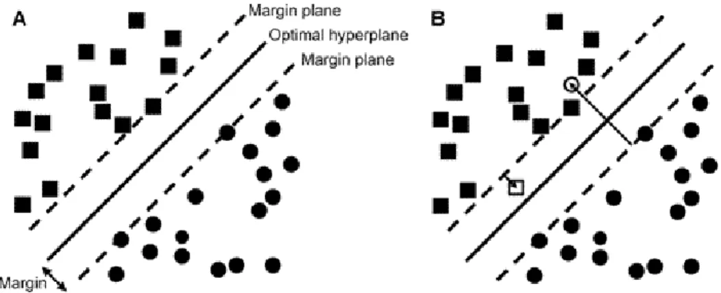
effec-tively on both linear and non-linear problems. The SVM creates a hyper-plane to split the data as accurately as possible, as shown in Figure 2.4. This is not a simple linear separation as by use of a kernel-trick the SVM transforms the feature space of descriptors. The linear hyperplane actually represents a nonlinear relationship of the data. This transformation is one of the problems of interpreting the model. Each kernel produces a different transformed feature space and thus several should be applied to find the op-timal kernel. In addition to selecting the most appropriate kernel there are various other parameters that should be optimised. Some parameters affect the kernel; others do not. Non kernel specific parameters of importance are the complexity constant andǫ. The complexity constant controls the toler-ation of misclassified instances, the higher the value the fewer misclassified instances are permitted. ǫ controls the round off value. Both these param-eters can greatly affect the model generated. The SVM implementation in Weka uses sequential minimal optimization variant of SVM to reduce the time consuming quadratic programming step.70,71

(49)

Figure 2.4: Separating hyperplane of the Support Vector Machine that max-imizes the margin between two sets of perfectly separable objects, repre-sented as circles and squares. (A) Optimal hyperplane that perfectly sepa-rates the two classes of objects. (B) Optimal soft margin hyperplane which tolerates some points (unﬁlled square and circle) on the wrong side of the appropriate margin plane. Reproduced with permission from Jorissen, R. N.; Gilson, M. K. Virtual Screening of Molecular Databases Using a Sup-port Vector Machine. J. Chem. Inf. Model. 2005, 45, 549-561 Copyright 2005 American Chemical Society

2.1.8

Partial Least Squares

PLS72 _{is the more advanced version of Principal Component Regression}

(PCR). PCR is concerned with explaining the variation in the dependent variable. PLS improves PCR by taking both the dependent and independent variables into account to explain the variation. PLS is a popular technique in both cheminformatics and chemometrics. PLS produces an equation which explains the dependent variable in terms of latent variables. These latent variables are the combination of the independent variables with a weighting coeﬃcient. The dependent variable,y, can be written as:

y=a1t1+a2t2 +a3t3+...antn (2.3)

wherean are coeﬃcients of the latent variables, tn. tn is deﬁned as

tn=bi1x1+bi2x2+...bipxp (2.4)

(50)

Each latent variable is orthogonal to each other, providing maximum variation from the previous. The maximum number of latent variables is the lower of the number of variables or instances. Typically, one will only use a handful of the total latent variables. The coeﬃcients, an, are of

interest as they eﬀectively weight or select the important features for the model. NCW uses these coeﬃcients to help identify what partial activity each atom provides when using the TMACC descriptors.

2.2

Model statistics

There are various statistics to assess the predictive performance of a model. Classification and regression tasks require different statistics. As we deal with both, both are presented here. The general paradigm for creating a model is to select a training set to build the model upon. That model is then used to predict unseen data from a test set. For techniques which require parameter optimisation, one may tune the model on a third, unseen, validation set, therefore giving the model new data at each stage. The abundance of data can be a luxury not afforded to all. Cross-validation can be used to assess the model by splitting the data in multiple training and test sets. Even if sufficient data are available, the statistics produced from cross validation are commonly used to compare models.

2.2.1

Classification

The initial statistics from a classiﬁcation experiment are the accuracy of the classiﬁcations. This leads to four numbers per class: true positive (T P), false positive (F P), true negative (T P) and false negative (F N). These four values are found in a confusion matrix. The number of classes determines the size of the matrix. A general confusion matrix is shown in Table 2.1. Knowing the incorrect predictions is perhaps more important than knowing

(51)

Actual Active Inactive

Predicted Active TP FP

Inactive FN TN

Table 2.1: A general confusion matrix

what was correct. It is useful to see what instances proved a challenge for the model to classify. A single statistic of use is the percentage of correctly classiﬁed instances. However, this only reports the correct and incorrect percentages, it does not take into account the four possible results (T P,

F P,T P,F N). This limitation does not apply to the Matthews correlation coeﬃcient,73 _{which takes all four into account, see Equation 2.5. Arguably}

the percentage of classiﬁed instances is an inferior statistic compared to the Matthews correlation coeﬃcient.

M CC = p T P ×T N −F P ×F N

(T P +F P) (T P +F N) (T N+F P) (T N +F N) (2.5) The value represents a perfect prediction for +1, average random for 0 and an inverse prediction for -1. A limitation of the MCC is that it only applies to binary classiﬁcation. For a greater number of classes one can use the Kappa coeﬃcient. Fleiss’ Kappa74_{not Cohen’s Kappa}75 _{is used, as the}

latter is for two classes only.

κ= P¯−P¯e 1₋P¯e

(2.6) where 1₋P¯eis the degree of agreement attainable above chance. ¯P−P¯eis the

degree of agreement actually achieved above chance. Complete agreement givesκ of one. When there is no agreement κ is below zero. ¯P is the mean of Pi and ¯Pe requires Pj. Pj, the proportion of all assignments which were

(52)

pj = 1 N n N