The LIBOR Market Model
Nevena ˇ
Seli´c
School of Computational and Applied Mathematics
University of the Witwatersrand
A dissertation submitted for the degree of
Master of Science in
Advanced Mathematics of Finance
Declaration
I declare that this is my own, unaided work. It is being submitted for the Degree of Master of Science to the University of the Witwatersrand, Johannesburg. It has not been submitted before for any degree or examination to any other University.
(Signature)
(Date)
Acknowledgements
The financial assistance of the National Research Foundation (NRF) towards this research is hereby acknowledged. Opinions expressed, and conclusions arrived at, are those of the author and are not necessarily to be attributed to the NRF.
I would like to thank my supervisor Professor David Taylor for his help, encouragement and support in writing this dissertation. I would also like to thank my friend Jacques du Toit for his comments and suggestions.
Nevena ˇSeli´c May 2006
Table of Contents
1 Introduction 1
2 LIBOR Market Model Theory 3
2.1 Theory of Derivative Pricing . . . 5
2.1.1 Model of the Financial Market . . . 5
2.1.2 Equivalent Martingale Measures . . . 7
2.1.3 Construction of Equivalent Measures . . . 9
2.1.4 Arbitrage-free Pricing . . . 12
2.1.5 Market Completeness . . . 13
2.2 LIBOR Market Model Theory . . . 13
2.2.1 Brace-G¸atarek-Musiela Model . . . 14
2.2.2 Forward Measures . . . 16
2.2.3 Discrete-tenor LIBOR Market Model . . . 18
2.2.4 Arbitrage-free Interpolation . . . 21
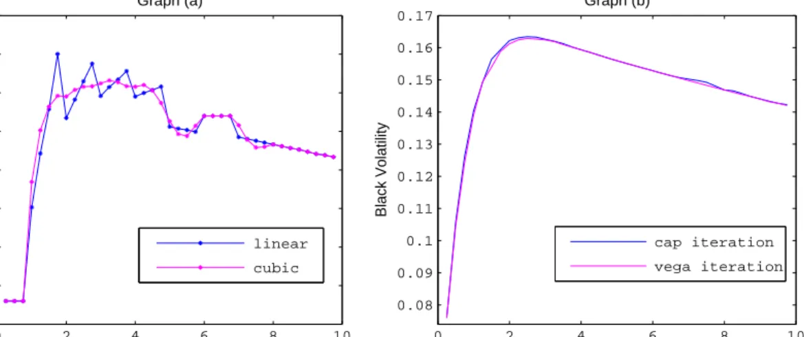
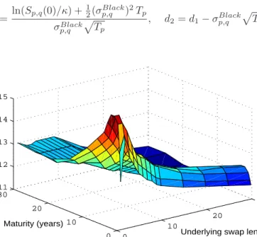
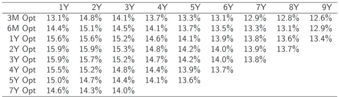
3 Calibration of the LIBOR Market Model 23 3.1 Model Dimension . . . 24 3.2 Rank Reductions . . . 25 3.2.1 Numerical Comparison . . . 28 3.3 Calibration Instruments . . . 29 3.3.1 Yield Curve . . . 29 3.3.2 Cap Volatilities . . . 30 3.3.3 Swaption Volatilities . . . 34 3.4 Model Choice . . . 36 3.4.1 Market Calibration . . . 39
4 Monte Carlo Basics 41 4.1 Monte Carlo Methods . . . 41
4.2 Low-Discrepancy Sequences . . . 42
4.2.1 Sobol’ Sequences . . . 44
4.3 Effective Dimension . . . 45
4.3.1 Brownian Bridge Construction . . . 46
4.4 Discretizations of the LIBOR Market Model . . . 47
4.4.1 Arbitrage-free Discretization . . . 48
4.4.2 Predictor-Corrector Method . . . 49
4.5 Numerical Results . . . 49
5 American Options 51
5.1 Primal and Dual Problem Formulations . . . 52
5.2 Parametric Early Exercise Boundary . . . 54
5.2.1 Application: Bermudan Swaption Pricing . . . 55
5.3 Parametric Continuation Value . . . 57
5.3.1 Parametric Regression . . . 57
5.3.2 Least Squares Monte Carlo . . . 57
5.4 Nonparametric Continuation Value . . . 59
5.4.1 Paradigms of Nonparametric Regression . . . 59
5.4.2 Penalized Regression Splines . . . 61
5.5 Dimension Reduction . . . 63
5.5.1 Sliced Inverse Regression . . . 63
5.6 Numerical Results . . . 64
Appendices 65
A Proof of Theorem 2.1.1 66
Chapter 1
Introduction
The over-the-counter (OTC) interest rate derivative market is large and rapidly developing. In March 2005, the Bank for International Settlements published its “Triennial Central Bank Survey” which examined the derivative market activity in 2004 (http://www.bis.org/publ/rpfx05.htm). The reported total gross market value of OTC derivatives stood at $6.4 trillion at the end of June 2004. The gross market value of interest rate derivatives comprised a massive 71.7% of the total, followed by foreign exchange derivatives (17.5%) and equity derivatives (5%). Further, the daily turnover in interest rate option trading increased from 5.9% (of the total daily turnover in the interest rate derivative market) in April 2001 to 16.7% in April 2004. This growth and success of the interest rate derivative market has resulted in the introduction of exotic interest rate products and the ongoing search for accurate and efficient pricing and hedging techniques for them.
Interest rate caps and (European) swaptions form the largest and the most liquid part of the interest rate option market. These vanilla instruments depend only on the level of the yield curve. The market standard for pricing them is the Black (1976) model. Caps and swaptions are typically used by traders of interest rate derivatives to gamma and vega hedge complex products. Thus an important feature of an interest rate model is not only its ability to recover an arbitrary input yield curve, but also an ability to calibrate to the implied at-the-money cap and swaption volatilities. The LIBOR market model developed out of the market’s need to price and hedge exotic interest rate derivatives consistently with the Black (1976) caplet formula. The focus of this dissertation is this popular class of interest rate models.
The fundamental traded assets in an interest rate model are zero-coupon bonds. The evolution of their values, assuming that the underlying movements are continuous, is driven by a finite number of Brownian motions. The traditional approach to modelling the term structure of interest rates is to postulate the evolution of the instantaneous short or forward rates. Contrastingly, in the LIBOR market model, the discrete forward rates are modelled directly. The additional assumption imposed is that the volatility function of the discrete forward rates is a deterministic function of time. In Chapter 2 we provide a brief overview of the history of interest rate modelling which led to the LIBOR market model. The general theory of derivative pricing is presented, followed by a exposition and derivation of the stochastic differential equations governing the forward LIBOR rates.
The LIBOR market model framework only truly becomes a model once the volatility functions of the discrete forward rates are specified. The information provided by the yield curve, the cap and the swaption markets does not imply a unique form for these functions. In Chapter 3, we examine various specifications of the LIBOR market model. Once the model is specified, it is calibrated to the above mentioned market data. An advantage of the LIBOR market model is the ability to calibrate to a large set of liquid market instruments while generating a realistic evolution of the forward rate volatility structure (Piterbarg 2004). We examine some of the practical problems that arise when calibrating the market model and present an example calibration in the UK market.
The necessity, in general, of pricing derivatives in the LIBOR market model using Monte Carlo simulation is explained in Chapter 4. Both the Monte Carlo and quasi-Monte Carlo simulation approaches are presented, together with an examination of the various discretizations of the forward rate stochastic differential equations. The chapter concludes with some numerical results comparing the performance of Monte Carlo estimates with quasi-Monte Carlo estimates and the performance of the discretization approaches.
pricing American derivatives. We present the primal and dual American option pricing problem formulations, followed by an overview of the two main numerical techniques for pricing American options using Monte Carlo simulation. Callable LIBOR exotics is a name given to a class of interest rate derivatives that have early exercise provisions (Bermudan style) to exercise into various underlying interest rate products. A popular approach for valuing these instruments in the LIBOR market model is to estimate the continuation value of the option using parametric regression and, subsequently, to estimate the option value using backward induction. This approach relies on the choice of relevant, i.e. problem specific predictor variables and also on the functional form of the regression function. It is certainly not a “black-box” type of approach.
Instead of choosing the relevant predictor variables, we present the sliced inverse regression technique. Sliced inverse regression is a statistical technique that aims to capture the main features of the data with a few low-dimensional projections. In particular, we use the sliced inverse regression technique to identify the low-dimensional projections of the forward LIBOR rates and then we estimate the continuation value of the option using nonparametric regression techniques. The results for a Bermudan swaption in a two-factor LIBOR market model are compared to those in Andersen (2000).
Chapter 2
LIBOR Market Model Theory
Mathematics possesses not only truth, but beauty - a beauty cold and austere, like that of a sculpture.– Bertrand Russell
The London Inter-Bank Offered Rates or LIBOR are benchmark short term simple interest rates at which banks can borrow money from other banks in the London interbank market. LIBOR rates are fixed daily by the British Bankers’ Association.1 They are quoted for various maturities
and currencies.
USD GBP CAD EUR JPY
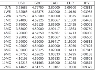
O/N 3.53688 4.79750 2.80000 2.09500 0.03813 1WK 3.62563 4.66375 2.80000 2.10150 0.03938 2WK 3.69250 4.60500 2.80000 2.10375 0.04000 1MO 3.74000 4.59125 2.80667 2.11300 0.04438 2MO 3.79000 4.59125 2.85500 2.12425 0.05063 3MO 3.85000 4.59000 2.90417 2.13363 0.05750 4MO 3.90000 4.57250 2.92667 2.14713 0.06000 5MO 3.95000 4.56063 2.95667 2.15038 0.06500 6MO 3.99000 4.55000 2.98417 2.15200 0.06813 7MO 4.02000 4.54000 3.00000 2.15950 0.07625 8MO 4.05000 4.53125 3.02000 2.16113 0.07813 9MO 4.07750 4.52625 3.03833 2.16725 0.08188 10MO 4.10163 4.52000 3.05833 2.17438 0.08563 11MO 4.12213 4.51563 3.08000 2.18288 0.08875 12MO 4.14625 4.51375 3.10167 2.19000 0.09375
Table 2.1: British Bankers’ Association LIBOR rate quotes on 9 September 2005 (source: Reuters) The LIBOR market model is an approach to modelling the term structure of interest rates based on simple rather than instantaneous rates. It was developed by Miltersen, Sandmann & Sondermann (1997), Brace, G¸atarek & Musiela (1997), Musiela & Rutkowski (1997) and Jamshid-ian (1997). However, this approach was certainly used by practitioners even before the first three references appeared as working papers in 1995. Quoting Rebonato (2002) on the LIBOR market model:
“. . . before any of the now-canonical papers appeared, it was simultaneously and in-dependently ‘discovered’ by analysts and practitioners who, undaunted by the ex-pected occurrence of the log-normal explosion, went ahead and discretized a log-normal forward-rate-based HJM implementation.”
We briefly trace the history of modelling the discretely compounded interest rates that led to the development of the LIBOR market model.
1
The rates are based on an arithmetic average of the offered interbank deposit rates - the deposit rates are ranked and the second and third quartiles are averaged to produce LIBOR rates (http://www.bba.org.uk).
In the early 1990’s, an important feature of an interest rate model was not only its ability to recover an arbitrary input yield curve, but also an ability to calibrate to the implied at-the-money cap and (European) swaption volatilities (Rebonato 2004). Caps and swaptions comprise the largest and the most liquid part of the interest rate derivative market. They are typically used by traders of interest rate derivatives to gamma and vega hedge complex products. The LIBOR market model developed out of the need to price and hedge exotic interest rate derivatives consistently with the Black caplet formula.
The traditional approach to modelling the term structure of interest rates was to postulate the evolution of instantaneous short or instantaneous forward rates. A tractable class of models, allowing “Black-like” closed-form formula for caplets, are the Gaussian instantaneous short rate and the Gaussian instantaneous forward rate models. An example of the former is the extended Vasicek model of Hull & White (1990), while an example of the latter is the Gaussian Heath, Jarrow & Morton (1992) (HJM) model developed by Brace & Musiela (1994). The problem with Gaussian models is that they lead to theoretical arbitrage opportunities - interest rates can become negative with positive probability. While the most natural way to exclude negative interest rates is through the lognormal distributional assumption, this too has difficulties. In the lognormal short rate models, such as Black, Derman & Toy (1990) and Black & Karasinski (1991), the expected value of the accumulation factors is infinite over a finite time horizon, i.e. EτB(t, T)−1=∞for
any 0≤τ < t < T, whereB(t, T) is the price attof a zero-coupon bond maturing atT (Sandmann & Sondermann 1997). The lognormal structure for the instantaneous forward rates leads to rates exploding to positive infinity with positive probability (Heath et al. 1992).
Sandmann & Sondermann (1993, 1994, 1997) noticed that the problems with the lognormal assumption arise as a consequence of modelling the instantaneous rates. The focus was shifted from modelling the instantaneous short rater(t) to modelling the effective annual ratere(t), defined by the formula er(t) = 1 +re(t). The authors proposed a binomial model for the effective annual
ratere(t), whose limiting dynamics are geometric Brownian motion with time dependent drift and volatility functions.2 For this limit model, the instantaneous short rater(t) follows a combination of
normal and lognormal diffusions - it approaches the lognormal diffusion for small values ofr(t) and a normal diffusion for large values ofr(t). Goldys, Musiela & Sondermann (1994, 2000) extended these results in the HJM framework. The specification of the volatility structure was shifted from the instantaneous forward ratesf(t, T) to ratesj(t, T) defined by the formulaef(t,T)= 1 +j(t, T).
A deterministic volatility function for the ratesj(t, T) was proposed and the authors proved that the resulting model has a unique positive solution, with no dreaded explosion of the instantaneous forward rates. The breakthrough came in Sandmann, Sondermann & Miltersen (1994), when the effective annual forward ratesfa(t, T, δ) at timetfor the interval [T, T +δ], defined by
1 +fa(t, T, δ)δ = exp
Z T+δ T
f(t, u)du
!
were modelled with a deterministic volatility function. It was shown that for δ = 1, closed-form solutions for zero-coupon bond options were computable. This exciting observation led to the Miltersen, Sandmann & Sondermann (1994, 1997) papers, where the simple forward ratesfs(t, T, δ) at timetfor the interval [T, T +δ], defined by
1 +δ fs(t, T, δ) = exp
Z T+δ T
f(t, u)du
!
were modelled with a deterministic volatility function. A closed-form expression for an option with exercise date T, written on a zero-coupon bond with maturity date T +δ, was obtained. In particular, caplets were priced according to the market standard Black caplet formula. Brace et al. (1997) derived the dynamics of the simple forward rates fs(t, T, δ) under the risk-neutral measure and proved the existence and uniqueness of a solution to the resulting stochastic differential equations.
An interest rate model implied by the assumption of a deterministic volatility function for the simple forward rates is known as the LIBOR market model (LMM) or the Brace-G¸atarek-Musiela (BGM) model. The construction of this model is presented in Section 2.2. In the following section we review the general theory of derivative pricing.
2
Suppose thatW is a standard Brownian motion and thatX satisfiesdX(t)/X(t) =µ(t)dt+σ(t)dW(t). We refer to µ(t) as the drift function and σ(t) as the volatility function. For a more general process X satisfying
2.1
Theory of Derivative Pricing
The history of modelling risky asset prices can be traced back to 1900, when French mathematician Louis Bachelier, under the supervision of Henri Poincar´e, proposed arithmetic Brownian motion for the movement of stock prices in his PhD thesis, “Th´eorie de la Sp´eculation”. To be more precise, 29 March 1900, the date on which Bachelier defended his thesis is considered to be the birth of mathematical finance (Courtault et al. 2000). The problem with Bachelier’s construction is that arithmetic Brownian motion is not a plausible model for asset prices because, amongst other things, it allows the asset prices to become negative. Sixty-five years later, Brownian motion was reintroduced in finance by Paul Samuelson in a paper written with Henry P. McKean Jr. (Samuelson 1965). Here he postulated that stock prices follow geometric Brownian motion, which circumvents the problems associated with Bachelier’s model.3
The breakthrough in derivative pricing came in the seminal papers of Black & Scholes (1973) and Merton (1973). The authors assumed geometric Brownian motion for the dynamics of the stock price and noted that a long position in a stock combined with a specific short position in a European call option on the stock will have a riskless return over an infinitesimally small period of time. To avoid arbitrage, the return must equal the prevailing risk-free rate. This observation led to the Black-Scholes partial differential equation for the derivative price, with explicit solutions for European call and put options. What is truly surprising about their result is the fact that a European option can be replicated by trading in the underlying stock and a riskless asset.
The Black-Scholes partial differential equation is independent of the expected return on the stock. This interesting property led to the discovery of risk-neutral valuation by Cox & Ross (1976). The concept was formalized and extended by Harrison & Kreps (1979) and Harrison & Pliska (1981, 1983). In accordance with J. Michael Harrison and Stanley R. Pliska’s seminal work, we now present the theory of derivative pricing in a frictionless market with continuous trading up to some fixed (finite) time horizonT.4
2.1.1
Model of the Financial Market
Consider a financial market with a fixed trading horizon [0, T]. The uncertainty in the economy is modelled by a filtered complete probability space Ω,F,F,P, where the filtrationF={Ft}0≤
t≤T satisfies the usual hypotheses.5 Assume that F
T = F and that F0 is trivial, i.e. for A ∈ F0,
P(A) ∈ {0,1}. The only role of a probability measureP is to determine the null sets. As the choice of a measure is arbitrary, the uncertainty in the economy can alternatively be modelled by a family of filtered probability spaces Ω,F,F,P, P ∈ P, where P is a class of equivalent
probability measures on Ω,FT (Musiela & Rutkowski 2005).6 The financial interpretation of
the assumption of a class P is that investors agree on which outcomes are possible, but their
probability assessments of these outcomes differ.
The financial market consists ofnprimary securities (traded assets). Denote the price process of the primary securities by S = {St,0≤t≤T}, where St = St1, . . . , Stn
′
. We model these
3
Jarrow & Protter (2004) provided a fascinating description of the history of stochastic integration. 4
To avoid inserting the same reference every few lines, we note that all the mathematical definitions in the following sections are taken directly from Protter (2004).
5
A filtered complete probability space (Ω,F,F,P) is said to satisfy theusual hypotheses if F0 contains all the
P-null sets ofF andFt=T
u>tFu, for all 0≤t < T. 6
Consider a measurable space (Ω,F) with measures Pand Qdefined on this space. Pisabsolutely continuous
with respect toQ, writtenP≪Q, ifP(A) = 0 wheneverQ(A) = 0 for allA∈F. IfP<<QandQ<<P, written
processes as strictly positive continuous semimartingales. A semimartingale, to be defined below, is the most general stochastic process for which the stochastic integral can be reasonably defined (Bichteler 1981). The semimartingale model is also quite a natural assumption, as it can be shown that, loosely speaking, the semimartingale model for asset prices is implied by the existence of an equivalent martingale measure (Delbaen & Schachermayer 1994b, Theorem 7.2). In this general model, both the arrival of random market information and deterministic components, such as the pull-to-par effects of zero-coupon bonds, can be incorporated. We now define these two components mathematically, followed by the definition of a semimartingale.
Definition 2.1.1. An adapted, c`adl`ag process M = {Mt,0≤t≤T} is a local martingale if
there exists a sequence of stopping times Tm, withlimm→∞Tm=T, almost surely, such that the
stopped process{Mt∧Tm,0≤t≤T} is a uniformly integrable martingale for eachm.
7
Definition 2.1.2. An adapted, c`adl`ag processA={At,0≤t≤T}is afinite variation process
if, almost surely, the paths ofAhave finite variation on each compact interval of[0, T].
Definition 2.1.3. An adapted, c`adl`ag processX ={Xt,0≤t≤T}is asemimartingaleif there
exist processesM,A withM0=A0= 0 such that
Xt=X0+Mt+At (2.1)
whereM is a local martingale andA is a finite variation process.
Decomposition (2.1) is not always unique because there exist finite variation martingales. IfXis a continuous semimartingale, then the decomposition is unique, and then both the local martingale and the finite variation process in the decomposition are continuous (Protter 2004, page 130).
In addition to the primary securities in the market, we have a European contingent claim maturing at time T that we want to price and hedge.8 The payoff of the contingent claim may
depend on the entire path of the primary securities up to and including the option maturityT. Thus, the contingent claim is modelled as a nonnegative,FT-measurable random variableϑ.
The pricing and hedging of contingent claims is based on the concept of a replicating portfolio. Suppose that we can construct a trading strategy, using the primary securities, which requires no cash inflow or outflow, except at inception, such that the final value of this portfolio matches the value of the contingent claim for allω ∈Ω almost surely. Then, by no-arbitrage arguments, the value of the contingent claim must equal the value of the portfolio at inception.
To formulate the contingent claim pricing problem formally, we need to define predictable and locally bounded processes. These technical assumptions are sufficient to ensure that the stochastic integral of a process satisfying these restrictions, with respect to a semimartingale, exists.
Definition 2.1.4. Let L denote the space of adapted processes with c`agl`ad (left continuous with right limits) paths. The predictable σ-algebra P on [0, T]×Ω is P = σ{X : X ∈ L}, the σ-algebra generated by all the processes inL. A process ispredictableif it is measurable with respect toP.
Definition 2.1.5. A process X={Xt,0≤t≤T}is said to belocally bounded if there exists a
sequence of stopping timesTm, withlimm→∞Tm=T, almost surely, such that the stopped process
{Xt∧Tm,0≤t≤T} is bounded for eachm.
Definition 2.1.6. An adapted n-dimensional stochastic process φ = {φt,0 ≤ t ≤ T}, where φt= φ1t, . . . , φnt
′
, is atrading strategyif φis locally bounded and predictable.
A trading strategyφtrepresents the number of assets held at timet, which is revised continu-ously through time. In a frictionless market, any quantity of assets can be both bought and sold at zero cost. The assumption that the processφis predictable has a financial interpretation: one establishes the portfolio just before timetand rebalances after the prices of the primary securities at timethave been observed. The assumption that a predictable processφis locally bounded has two implications. Firstly, the stochastic integral of a locally bounded (predictable) process with
7
A stochastic process X={Xt,0≤t≤T}is said to beadapted ifXt ∈Ft for eacht∈[0, T]. It isc`adl`ag if it almost surely has sample paths which are right continuous with left limits. The process isuniformly integrableif limm→∞sup0≤t≤T
R
|Xt|≥m|Xt|dP= 0.
8
Risk-neutral valuation of American derivatives was developed by Bensoussan (1984) and Karatzas (1988, 1989). The American option pricing problem will be formulated in Chapter 5.
respect to a local martingale is itself a local martingale, a statement that is not true in general (Protter 2004, page 171). Secondly, the stochastic integral can be defined component-wise, that is the stochastic integral of a trading strategy with respect to a semimartingale is equal to the sum of the stochastic integrals of the relevant vector components (cf. equation (2.3) below) (Musiela & Rutkowski 2005, page 281).
Associated with each trading strategy φ is the value process V(φ) = {Vt(φ),0 ≤ t ≤ T}, defined by Vt(φ) =φt·St= n X i=1 φitSti, (2.2)
Assuming that the primary securities do not generate any cashflows such as dividends, thegains process G(φ) ={Gt(φ),0≤t≤T}is defined by Gt(φ) = Z t 0 φu·dSu= n X i=1 Z t 0 φi udSiu, (2.3)
The gains process is adapted and continuous, because it is a stochastic integral with respect to a continuous semimartingale. It represents the total capital gain when trading strategyφis followed. A trading strategy that requires no external cashflows is termed a self-financing trading strategy.
Definition 2.1.7. Aself-financing trading strategyis a trading strategyφwhose value process satisfies
Vt(φ) =V0(φ) +Gt(φ), 0≤t≤T (2.4)
Equation (2.4) can be written in a more familiar form asd(φt·St) =φt·dSt. Note that the self-financing condition ensures that the value process is continuous.
Let us restate the pricing problem in terms of the introduced notation: we are looking for a self-financing trading strategyφsuch thatVT(φ) =ϑ, almost surely. If we can find such aφ, then by no-arbitrage arguments, the value of the claim at any timetmust beVt(φ). However, it turns out that one cannot naively allow all self-financing trading strategies. There are two problems that need to be addressed. Firstly, we need to remove doubling strategies that turn “nothing into something” because they represent arbitrage opportunities. A classical example of a doubling strategy is the coin toss game, where if heads comes up, the payout is two times the bet amount. A player bets one unit of currency on the first bet and if he looses he doubles his bet. The player stops at the time of the first win, which is inevitable, even if the coin is not fair. However, one needs to be able to fund arbitrarily large losses until the eventual win. It is possible to construct these strategies in the current framework because trading takes place continuously, and hence infinitely many times in the interval [0, T].9 Secondly, we need to remove suicide strategies that turn “something into
nothing” because they lead to non-unique pricing. If suicide strategies are permitted, one may find two self-financing trading strategies for a claim whose value processes have different initial values.10 The necessary modifications to a class of self-financing trading strategies depend on the
notion of an equivalent martingale measure.
2.1.2
Equivalent Martingale Measures
At the heart of mathematical finance is the assumption that there are no arbitrage opportunities in well-functioning markets.
Definition 2.1.8. A self-financing trading strategyφis called an arbitrage opportunityif the value process satisfies the following set of conditions
V0(φ) = 0, P(VT(φ)≥0) = 1, P(VT(φ)>0)>0
The “no-arbitrage pricing” approach postulates that there are no arbitrage opportunities in the market. In the Black-Scholes model, the assumption of an arbitrage-free market implies, and is implied by, the existence of a unique equivalent measure such that the stock prices normalized by the money-market account are martingales under this measure. In the general framework one needs to choose an asset, called the num´eraire, to normalize the other assets in the market.
9
For an example of a doubling strategy in the Brownian motion setting, see Duffie (1996, Chapter 6.C). 10
Definition 2.1.9. A num´eraire is a price process X ={Xt,0≤t≤T} that is, almost surely,
strictly positive for allt∈[0, T].
All the price processes of the primary securities are strictly positive by assumption. Without loss of generality, choose securityS1 to be the num´eraire.11 Thedeflator process Y ={Y
t,0≤t≤T} is a strictly positive semimartingale, defined byYt = 1/St1 through Itˆo’s formula for continuous semimartingales (Karatzas & Shreve 1991, page 149). Thenormalized asset price processis denoted by Z = {Zt,0≤t≤T}, where Zt = 1, Zt2, . . . , Ztn
′
and Zi
t = YtSti for i = 1, . . . , n. The
normalized value process V∗(φ) and the normalized gains process G∗(φ) of a trading strategy φ are defined by Vt∗(φ) = YtVt(φ) =φt·Zt=φ1t+ n X i=2 φitZti, 0≤t≤T (2.5) G∗t(φ) = Z t 0 φu·dZu= n X i=1 Z t 0 φiudZui = n X i=2 Z t 0 φiudZui, 0≤t≤T (2.6) Self-financing trading strategies were defined as trading strategies whose value processes satisfy equation (2.4). To show that self-financing trading strategies remain self-financing after a num´eraire change, we need to define the quadratic covariation process.
Definition 2.1.10. LetX andY be semimartingales. Thequadratic covariationofX,Y, also called the(square) bracket process, is defined by
[X, Y]t=XtYt− Z t 0 Xu−dYu− Z t 0 Yu−dXu (2.7)
whereX−(Y−)is the left-continuous version ofX(Y). The quadratic variationof X is[X, X].
Equation (2.7) is also known as the integration by parts formula. To obtain a better under-standing of the quadratic covariation process, supposeX andY are continuous local martingales. Then the process
XtYt−[X, Y]t= Z t 0 XudYu+ Z t 0 YudXu
is a continuous local martingale. Heuristically,d[X, Y]tis the conditional expectation just beforet
ofd(XY)t(Back 2001). For a standard Brownian motionW, which is a continuous local martingale, we know that [W, W]t=tfor allt≥0.
Consider a self-financing trading strategyφ. We now show that self-financing trading strategies remain self-financing after a num´eraire change, i.e. thatd(φt·Zt) =φt·dZt.
d YtVt(φ) = YtdVt(φ) +Vt(φ)dYt+d[Y, V(φ)]t = Yt(φt·dSt) + (φt·St)dYt+d[Y,φ·S]t = φt· YtdSt+StdYt+d[Y,S]t = φt·d(YtSt) Thus Vt∗(φ) =V0∗(φ) +G∗t(φ), 0≤t≤T (2.8) Substituting equations (2.5) and (2.6) into (2.8), we see thatφ1can be used to form a self-financing
trading strategy from an arbitrary trading strategyφ, by setting
φ1t =V0∗(φ) + n X i=2 Z t 0 φiudZui − n X i=2 φitZti, 0≤t≤T
LetP∗ be the set (possibly empty) of equivalent martingale measures, defined as a set of
equiva-lent measures such that, forP∗∈P∗, the normalized asset pricesZareP∗-martingales. The link
between equivalent martingale measures and the absence of arbitrage is known as theFundamental Theorem of Asset Pricing. This theorem states that, for a stochastic processZ, the existence of
11
In the general equity market setting, securityS1
an equivalent martingale measure is essentially equivalent to the absence of arbitrage opportuni-ties (Delbaen & Schachermayer 1994b). It is extremely difficult to prove the exact mathematical conditions that the normalized asset price processZneeds to satisfy for the absence of arbitrage to imply the existence of an equivalent martingale measure. These restrictions have been estab-lished in a series of papers by Delbaen (1992) and Delbaen & Schachermayer (1994a,b, 1998), for increasingly general classes of processes. We will assume thatP∗ is non-empty and examine the
reverse implication of the existence of an equivalent martingale measure implying the absence of arbitrage opportunities.
To remove the doubling strategies discussed in the previous subsection, one can require that the value processes be bounded from below. Harrison & Pliska (1981) defined Φ as a class of self-financing trading strategiesφwhose value process satisfies
Vt(φ)≥0, 0≤t≤T
Forφ∈Φ, the normalized value processV∗(φ) is also nonnegative. This is due to the fact that
the deflator is a strictly positive process. Note thatφ1 can still be used appropriately to define a
self-financing trading strategy, as long as the constructed normalized value process is nonnegative. In order to eliminate suicide strategies, Harrison & Pliska (1981) fixed a measure P∗ ∈ P∗
and defined a class ofadmissible trading strategies Φ(P∗) as self-financing trading strategiesφ∈Φ
whose normalized value processesV∗(φ) areP∗-martingales. This restriction is sufficient to remove
suicide strategies because due to the martingale property,V∗
T(φ) cannot be zero, almost surely, if
V∗
0(φ) is positive.
Theorem 2.1.1. Assume thatP∗ is non-empty. Then the model is arbitrage-free. Proof. The proof is given in Appendix A.
The question that we now address is, “How do we construct an equivalent martingale measure P∗ when dealing with semimartingale processes?”
2.1.3
Construction of Equivalent Measures
In this section we examine the construction of a probability measureQon (Ω,FT) that is equivalent
to the underlying probability measure P. Following Protter (2004), we know that if Q ≪ P, there exists a nonnegativeP-integrable random variableζT, called theRadon-Nikod´ym derivative, satisfyingEP[ζ
T] = 1, such that for all A∈FT Q(A) =
Z
A
ζTdP
The Radon-Nikod´ym derivativeζT is denoted by ddQP. The Radon-Nikod´ym derivative process is the c`adl`ag version of the following uniformly integrable martingale12
ζt=EP[ζT|Ft], 0≤t < T (2.9) IfP≪Qas well, then dP dQ = dQ dP −1
. Thus if we can construct the Radon-Nikod´ym derivative, we can construct an equivalent probability measure.
The construction of an equivalent probability measure when the underlying processes are semi-martingales is due to Christopeit & Musiela (1994). Note that in general, even if the underlying processes are continuous semimartingales, the Radon-Nikod´ym derivative process may be discon-tinuous because the underlying filtration is not necessarily Brownian (Musiela & Rutkowski 2005, page 295). We now introduce the Dol´eans-Dade exponential.
Definition 2.1.11. TheDol´eans-Dade exponentialE(D)is the unique solution of the stochas-tic differential equation
dE(D)t=E(D)t−dDt, E0(D) = 1 (2.10)
The explicit solution to (2.10) is given by E(D)t= exp Dt− 1 2[D, D] c t Y 0≤u≤t (1 + ∆Du)e−∆Du (2.11) 12
One of the consequences of the usual hypotheses is that every martingale has a version that is c`adl`ag (Protter 2001).
where∆Dt=Dt−Dt− and[D, D]c is the path-by-path continuous part of the quadratic variation process[D, D] [D, D]ct= [D, D]t− X 0≤u≤t (∆Du)2
Theorem 2.1.2. ConsiderQ∼Pand the Radon-Nikod´ym derivative process ζ, as defined. Sup-pose that there exists aP-local martingale D withD0=D0−= 0 satisfying
∆Dt>−1, 0≤t≤T (2.12)
EP[E(D)T] = 1 (2.13)
where∆Dt=Dt−Dt−andE(D)is the Dol´eans-Dade exponential. Then there exists a one-to-one correspondence betweenζ andD, given by
ζt=E(D)t, 0≤t≤T
Theorem 2.1.2 states that the Radon-Nikod´ym derivative process is the Dol´eans-Dade exponen-tial of a local martingale satisfying certain conditions. Firstly, condition (2.12) is a condition on the jump sizes. From equation (2.11), it is easily seen that this restriction makes the Dol´eans-Dade exponential strictly positive. Secondly, the Dol´eans-Dade exponential is a uniformly integrable martingale if and only if condition (2.13) is satisfied.
Girsanov’s Theorem, also known as the Girsanov-Meyer Theorem, provides us with the semi-martingale decomposition under an equivalent probability measureQ.
Theorem 2.1.3. Let X be a continuous semimartingale underP with the decomposition Xt=X0+Mt+At, 0≤t≤T
whereM is a continuous local martingale andAis a continuous finite variation process. Let Qbe an equivalent measure and let the Radon-Nikod´ym derivative dQ
dP be defined by the Dol´eans-Dade
exponential of a local martingaleD (cf. Theorem 2.1.2). SinceM has bounded jumps(∆Mt= 0),
the cross-variation processhM, Diexists (Christopeit & Musiela 1994, Corollary 1).13 Then X is a continuous semimartingale underQwith the decomposition
Xt=X0+Lt+Ct, 0≤t≤T (2.14)
whereLis aQ-local martingale
Lt=Mt− hM, Dit, 0≤t≤T
andC is aQfinite variation process
Ct=At+hM, Dit, 0≤t≤T
In particular,X is a local martingale underQif and only if
At+hM, Dit= 0, 0≤t≤T (2.15)
The Black-Scholes Model
The two theorems presented above can be made more intuitive in the familiar framework of Black and Scholes. The normalized asset price processZ is the discounted stock price process. UnderP,
Z satisfies
dZt= (µ−r)Ztdt+σZtdWt (2.16)
whereµis the expected return on the asset,σis the return volatility,ris the risk-free continuously compounded rate of interest andW is a standard Brownian motion. The parametersµ, r andσ
are constants. The Martingale Representation Theorem (Karatzas & Shreve 1991, Theorem 4.2) is a beautiful result that demonstrates how one can represent martingales in terms of Brownian motion, a fundamental continuous martingale.
13
Thecross-variation processhX, Yi, also called theconditional quadratic covariation, is defined to be the com-pensator of [X, Y], i.e. a unique predictable finite variation process such that [X, Y]− hX, Yiis a local martingale. IfX andY are continuous semimartingales, [X, Y] =hX, Yi.
Theorem 2.1.4 (Martingale Representation Theorem). Suppose W= (W1, . . . , Wn)′ is a n-dimensional Brownian motion and let FW be its completed natural filtration. Then every continuous local martingaleM for FW has a representation
Mt=M0+ n X i=1 Z t 0 Hi udWui
whereHi are measurable adapted processes satisfying PhRt
0 H
i u
2
du <∞i= 1for all 0 ≤t≤T and i = 1, . . . , n. Further, if L and N are two continuous local martingales for FW with the
representations Lt=L0+ n X i=1 Z t 0 HuidWui Nt=N0+ n X i=1 Z t 0 e HuidWui whereHi
u andHeui satisfy the condition stated above, then
hL, Nit= n X i=1 Z t 0 HuiHeuidu (2.17)
In the Black-Scholes model, the underlying filtration is the augmented filtration generated by the Brownian motionW. In particular, this implies that the Radon-Nikod´ym derivative process is a continuous martingale. From the Martingale Representation Theorem
ζt= 1 +
Z t
0
HudWu whereζ0= 1, due to the conditionEP[ζ
T] = 1. Following Protter (2004), we assume thatζis “well behaved enough” to define a process λ={λt,0 ≤t ≤ T} through the formula Ht =λtζt. The dynamics ofζbecome
dζt
ζt
=λtdWt (2.18)
The explicit solution of the stochastic differential equation (2.18) is
ζt= exp −12 Z t 0 λ2udu+ Z t 0 λudWu (2.19) Theorem 2.1.2 states that the Radon-Nikod´ym derivative process is the Dol´eans-Dade exponential of a local martingaleDsatisfying conditions (2.12) and (2.13). It follows from equation (2.19) that the local martingaleD is given by Dt=R0tλudWu. This can easily be verified: the jump sizes of the continuous processD are zero, ∆Dt= 0, and the Dol´eans-Dade exponential ofD is
E(D)t = exp Z t 0 λudWu−1 2[D, D]t = exp Z t 0 λudWu−1 2 Z t 0 dDudDu = exp Z t 0 λudWu− 1 2 Z t 0 λ2udu Hence EP[E(D)T] = exp −1 2 Z T 0 λ2udu ! EP " exp Z T 0 λudWu !# = 1
The last equality follows from the fact that if a random variableX is normally distributed with mean µ and variance σ2, written X
EetX=eµt+1 2σ
2t2
. The mean of the normal random variableR0TλudWu is zero, because an Itˆo integral is a martingale, while the variance ofR0TλudWu isR0Tλ2udu, by Itˆo isometry.
In particular, from Theorem 2.1.2, the local martingale Dt =R t
0λdWu defines an equivalent
probability measure for any constantλ ∈ R. What we are really interested in is an equivalent martingale measure. For this we turn to Theorem 2.1.3.
The normalized asset price processZ is an Itˆo process and hence a continuous semimartingale underP. In particular, using the notation of Theorem 2.1.3, we haveZ=Z0+Mt+At where
Mt= Z t 0 σZudWu and At= Z t 0 (µ−r)Zudu
For an equivalent probability measureQ to be an equivalent martingale measure, Z must be a Q-martingale. Theorem 2.1.3 states that Z is a local martingale underQif and only if
At+hM, Dit= 0 Substituting in forA,M andD, and using equation (2.17)
Z t 0 (µ−r)Zudu+ Z t 0 σZuλudt= 0 ⇒ (µ−r)Ztdt+σZtλtdt= 0 ⇒ λt=−µ−r σ
Given this choice ofλt, theQ-local martingaleZ has the decompositionZ=Z0+Lt, where
Lt = Mt− hM, Dit = Z t 0 σZudWu− Z t 0 σZu −µ−σ r du = Z t 0 σZudWu+ Z t 0 (µ−r)Zudu = Z t 0 σZu dWu+µ−r σ du
is aQ-local martingale. Following Protter (2004), let
dWuQ=dWu+
µ−r σ du
denote this local martingale. By L´evy’s Theorem,WQ is Brownian motion because
hWQ, WQ
it=
hW, Wit=t. UnderQ,Z satisfies
dZt=σZtdWtQ
Asσ is a constant, hence bounded,Z is aQ-martingale. Thus, as expected, only whenλt is the negative of the market price of risk doesDt=R0tλudWudefine an equivalent martingale measure.
2.1.4
Arbitrage-free Pricing
A contingent claim ϑ is said to be attainable if there exists φ ∈ Φ(P∗) such that V
T(φ) = ϑ. Assuming that the random variableYTϑisP∗-integrable (termedintegrable claim), the arbitrage-free price of the attainable contingent claimϑis given by
Vt(φ) = 1 Yt Vt∗(φ) = 1 Yt EP∗[VT∗(φ)|Ft] = 1 Yt EP∗[YTϑ|Ft]
for all 0≤t≤T. This is the fundamental pricing equation: the normalized contingent claim price
Theorem 2.1.5. Suppose that the contingent claim ϑ is attainable in P∗1 ∈ P∗ and P∗
2 ∈ P∗. Then the arbitrage-free prices will be equal, i.e.
EP∗1[Y
Tϑ|Ft] =EP ∗ 2[Y
Tϑ|Ft], 0≤t≤T
Proof. The proof follows Musiela & Rutkowski (2005) and is given in Appendix B.
The question of whether every integrable claim is attainable, termed market completeness, depends on the class of admissible trading strategies.
2.1.5
Market Completeness
A market is referred to as complete if every integrable claim is attainable. Thus far, the trading strategies identified turn out to be too restricted if one wants to replicate all integrable claims. In particular, the assumption of locally bounded processes is problematic. Harrison & Pliska (1983) extended the set of trading strategies to a larger classL(Z), the set of vector-valued, predictable processes that are integrable with respect to a semimartingaleZ.14 The main result of Harrison &
Pliska (1981, 1983) follows.
Theorem 2.1.6. Let Zdenote the normalized asset price process and letM denote the set of all
P∗-martingales. Then the following statements are equivalent: 1. The market is complete under P∗.
2. Every martingaleM ∈M can be represented as M =M0+
Z
φ·dZ, for someφ∈L(Z)
3. P∗ is a singleton, i.e. there is only one equivalent martingale measure P∗∈P∗.
According to Protter (2001), few martingales possess the second property in the previous theo-rem. In fact, the only examples given in the paper are Brownian motion, the Compensated Poisson process and Az´ema martingales.
Theorem 2.1.6 shows that prefect hedging of a contingent claim is possible only if the integral representation of the normalized claim price (a martingale) exists. In particular, suppose that a contingent claimϑis integrable. Then ϑis attainable if the normalized claim price
Mt=EP ∗
[YTϑ|Ft], 0≤t≤T admits the integral representation
Mt=M0+ n X i=2 Z t 0 φiudZui, 0≤t≤T
In a complete market, the equivalent martingale measureP∗ is unique and every integrable claim is attainable. In an incomplete market, the problem of hedging non-attainable claims becomes one of selecting an equivalent martingale measure that is optimal in some sense. Musiela & Rutkowski (2005) provide a brief introduction to this active area of current research.
2.2
LIBOR Market Model Theory
In this section we construct the LIBOR market model under the assumption that there are no “smile effects” in the interest rate market. This means that the caplet and swaption implied volatility surfaces are assumed to be, for a fixed expiry, a flat function of the strike.15
14
Jarrow & Madan (1994) examined the distinction between vector- and component-wise stochastic integrals in the Brownian motion setting. They note that the earlier paper, Harrison & Pliska (1981), misspecified the class L(Z). The class implicitly assumed by Harrison & Pliska (1983), this being the set of vector-valued, predictable
processes that are integrable with respect to a semimartingaleZ, is the correct one for Theorem 2.1.6 to be valid. 15
2.2.1
Brace-G¸
atarek-Musiela Model
Motivated by the lack of an arbitrage-free term structure model consistent with the market practice of pricing caps and floors (which generally comprise the largest part of any interest rate derivative book), Brace et al. (1997) set out to construct such a model in the HJM framework. We provide an overview of the HJM framework, followed by details of the BGM construction of the market model.
Heath-Jarrow-Morton Framework. Heath et al. (1992) developed a framework for mod-elling the term structure of interest rates based on an exogenous specification of the evolution of the instantaneous forward rates. Interest rate modelling is assumed to take place in continuous time over the interval [0, T∗], on a probability space (Ω,F,P). The probability space is equipped
with a filtrationF={Ft}0≤t≤T∗, the augmented filtration generated by ad-dimensional Brownian motionW = W1, . . . , Wd′. Each component of the vector Brownian motionW represents an independent, exogenous source of uncertainty in the financial market.
Assumption (Heath et al. 1992, C.1). For fixed T ∈ [0, T∗] define the instantaneous, contin-uously compounded forward rate at timet for maturityT,f(t, T), by
f(t, T) =−∂T∂ logB(t, T)
whereB(t, T)is the price at tof a zero-coupon bond maturing atT. Then, under P, the instanta-neous forward ratesf(t, T)satisfy
df(t, T) =α(t, T, ω)dt+ d X i=1 σi(t, T, ω)dWti whereω∈Ωand
1. the initial forward rate curve,f(0,·) : [0, T∗]→Ris a Borel-measurable function,
2. α:{(t, s) : 0≤t≤s≤T} ×Ω→Rand σi :{(t, s) : 0≤t≤s≤T} ×Ω→Rare adapted
processes such that, almost surely,
Z T 0 | α(u, T, ω)|du+ Z T 0 | σi(t, T, ω)|2dt <∞, for i= 1, . . . , d
Some extra conditions are needed for the regularity of the zero-coupon bond price processes and the money-market account (Heath et al. 1992, C2 and C3). The money-market account is defined as B∗(t) = exp Z t 0 r(u)du (2.20) whereris the instantaneous, continuously compounded short rate,r(t) = limT→tf(t, T).
The primary securities are zero-coupon bonds of different maturities. Heath et al. (1992) identified the restrictions that the assumption of an arbitrage-free market imposes on the evolution of the term structure of interest rates. In particular, after constructing a portfolio consisting of a finite number of zero-coupon bonds, the authors derived the necessary and sufficient conditions on the drift of the instantaneous forward rates for the existence of a unique equivalent martingale measureQ, corresponding to the money-market account num´eraire. Under Q, the instantaneous forward ratesf(t, T) satisfy
df(t, T) =σ(t, T)·σ∗(t, T)dt+σ(t, T)·dWQt, σ∗(t, T) =
Z T t
σ(t, u)du (2.21) whereσ(t, T) = (σ1(t, T, ω), . . . , σd(t, T, ω))′andWQis ad-dimensionalQ-Wiener process. Under Q, the zero-coupon bond pricesB(t, T) satisfy
dB(t, T)
B(t, T) =r(t)dt−σ
∗(t, T)
·dWQt (2.22)
The assumption of no arbitrage implies that the drift coefficient of the instantaneous forward rates is uniquely determined once the diffusion coefficient is specified. This is in great contrast to in-stantaneous short rate models, where the drift coefficient can be specified independently of the
diffusion coefficient and is in fact used to calibrate the model to the initial yield curve. In the HJM framework, the initial condition for the stochastic differential equation (2.21) is the initial forward ratef(0, T). The calibration to the initial yield curve is automatic because the current yield curve is a function of the initial instantaneous forward rates,B(0, T) = exp(−R0Tf(0, u)du).
Brace-Gatarek-Musiela Construction. Brace et al. (1997) considered a simple interest rate defined over a finite accrual periodδ >0. Denote the simple forward rate at time t for the time interval [T, T +δ] byfs(t, T), for 0≤ t ≤T ≤T∗−δ. Using no-arbitrage arguments, the
simple forward ratesfs(t, T) are defined in terms of the zero-coupon bond prices 1 +δfs(t, T) = B(t, T)
B(t, T+δ) (2.23)
or, equivalently, in terms of the instantaneous forward rates 1 +δ fs(t, T) = exp Z T+δ T f(t, u)du ! (2.24) Brace et al. (1997) derived the dynamics of the simple forward rates under the equivalent martingale measureQusing the dynamics of the instantaneous forward rates. However, it is much easier to identify the dynamics of the simple forward rates using relationship (2.23) and equation (2.22).
Lemma 2.2.1. Suppose thatX and Y are two Itˆo processes satisfying dXt Xt =µXt dt+σXt dWt, dYt Yt =µYtdt+σtYdWt
where the adapted functionsµX
t , µYt , σXt andσYt satisfy the conditions needed for the existence and
uniqueness of strong solutions of the above stochastic differential equations.16 Then d X t Yt = X t Yt µXt −µYt dt+ σtX−σtY −σtYdt+dWt
The proof is a straightforward application of Itˆo’s formula. Applying this result in equation (2.23), together with equation (2.22), we see that underQ, the simple forward rates satisfy
dfs(t, T) = 1 δd B(t, T) B(t, T+δ) = δ−1 B(t, T) B(t, T +δ) σ∗(t, T +δ)−σ∗(t, T)·σ∗(t, T+δ)dt+dWQt = δ−1 1 +δfs(t, T) σ∗(t, T +δ)−σ∗(t, T)·σ∗(t, T+δ)dt+dWtQ (2.25) This is the HJM model for the simple forward ratesfs(t, T). Brace et al. (1997) postulated that the simple forward rates have a deterministic volatility function
dfs(t, T) =ζtdt+fs(t, T)λ(t, T)·dWQt (2.26) with some (to be determined) drift functionζtand a deterministic, bounded, piecewise continuous functionλ:R2+→Rd. The volatility functionλ(t, T) is exogenously specified.
The motivation for this assumption was the Black caplet formula. As we shall show in the following chapter, the assumption of a deterministic volatility function for the simple forward rates is consistent with the Black model, meaning that the resulting model caplet pricing formula agrees with the market standard Black caplet formula.
Equating the diffusion coefficients of equations (2.25) and (2.26), we obtain σ∗(t, T+δ)−σ∗(t, T) = δfs(t, T)
1 +δfs(t, T)λ(t, T) (2.27)
16
These conditions are measurability, Lipschitz condition, linear growth and the initial value condition (Kloeden & Platen 1999, Section 4.5).
To determineσ∗(t, T+δ), we can use as a recursion relationship (2.27) σ∗(t, T+δ) = σ∗(t, T) + δfs(t, T) 1 +δfs(t, T)λ(t, T) = σ∗(t, T−δ) + δfs(t, T −δ) 1 +δfs(t, T −δ)λ(t, T−δ) + δfs(t, T) 1 +δfs(t, T)λ(t, T) = σ∗(t, T−kδ) + k X j=0 δfs(t, T−jδ) 1 +δfs(t, T−jδ)λ(t, T−jδ)
wherek=Tδ−t andt ≤T −kδ < t+δ.17 To start the recursion one needs to assign values to
σ∗(t, T−kδ), this being the volatility function of zero-coupon bonds with maturities shorter than δ(cf. equation (2.22)). Brace et al. (1997) assumed thatσ∗(t, T) = 0 for 0≤T−t < δ. Then
σ∗(t, T+δ) = ⌊δ−1(T−t)⌋ X j=0 δfs(t, T−jδ) 1 +δfs(t, T −jδ)λ(t, T−jδ) (2.28) Substituting equations (2.27) and (2.28) in (2.25), we obtain the dynamics of the simple forward ratesfs(t, T) underQ dfs(t, T) =fs(t, T)λ(t, T)· ⌊δ−1(T−t)⌋ X j=0 δfs(t, T−jδ) 1 +δfs(t, T−jδ)λ(t, T−jδ)dt+dW Q t (2.29)
Brace et al. (1997) proved the existence and uniqueness of a solution to the stochastic differential equation (2.29). Note that in the BGM model, it is the forward rate volatility function λ(t, T) that is exogenously specified, not the zero-coupon bond price volatility functionσ∗(t, T).
The technical problem with this analysis is that in the HJM framework, the zero-coupon bond price volatility functionσ∗(t, T) has to be sufficiently smooth for the instantaneous forward rates to exist. From the definition of this function in equation (2.21), we see that it must be differentiable with respect toT. This restricts the choice of a deterministic simple forward rate volatility function
λ(t, T) because of its relationship with the zero-coupon bond price volatility function, equation (2.28). In particular, Brace et al. (1997) parameterized the simple forward rate volatility function as piecewise continuous, which is not a differentiable function. Thus, theoretically, the piecewise continuous specification cannot be analyzed in the HJM framework. As the assumption of the existence of instantaneous forward rates is not convenient, we now examine an alternate approach of modelling the zero-coupon bond price process without any reference to the instantaneous forward rates.
2.2.2
Forward Measures
The existence of a unique equivalent martingale measure Q associated with the money-market account num´eraire implies, and is implied by, an arbitrage-free and complete interest rate system. UnderQ, the value of any traded asset normalized by the money-market account is a martingale. Thus the current value of a traded asset is the expected value, underQ, of the discounted terminal asset value. This is the so-called risk-neutral valuation.
When pricing interest rate derivatives, it is frequently convenient to use a zero-coupon bond as a num´eraire.18 The measure associated with the zero-coupon bond maturing at timeT is called the T-forward measure. Geman, El Karoui & Rochet (1995) showed that the T-forward measureQT is a probability measure on Ω,FT, equivalent to Q, defined by the Radon-Nikod´ym derivative
dQT
dQ =
1
B(0, T)B∗(T)
where B∗ is the money-market account.19 Under QT, any traded asset normalized by the zero-coupon bond maturing at time T is a martingale. We can reformulate the opening statement as
17
⌊x⌋is the largest integer less than or equal tox. 18
For example, when an option has a payoff at timeT, it is convenient to use the zero-coupon bond maturing at timeT as the num´eraire because the value of this num´eraire atT is one. This avoids having to derive the joint distribution of the payoff and the num´eraire.
19
In an arbitrage-free and complete market there exists one equivalent martingale measure associated with each num´eraire.
follows: the existence of a unique equivalent martingale measure QT associated with the zero-coupon bond maturing at timeT as a num´eraire implies, and is implied by, an arbitrage-free and complete interest rate system.
A modern interest rate model consists of a num´eraire and a set of stochastic differential equa-tions that a family of zero-coupon bonds satisfy. Following Musiela & Rutkowski (1997), we define an interest rate system by imposing the following assumptions.
Assumption 1. The family of zero-coupon bond prices B(t, T), 0 < t ≤T ≤T∗, are modelled as strictly positive, continuous semimartingales. A deterministic initial term structure of interest ratesB(0, T),T ∈[0, T∗], is exogenously specified.
Assumption 2. There exists a unique equivalent martingale measure QT∗ such that for every T ∈[0, T∗), the forward process
F(t, T, T∗) = B(t, T)
B(t, T∗), 0≤t≤T is a strictly positive, continuous martingale underQT∗.
The first assumption is a fairly general specification of the zero-coupon bond price processes. We will further assume that the underlying filtration is Brownian (cf. Section 2.2.1). The second assumption implies that the interest rate system is arbitrage-free and complete.
By the Martingale Representation Theorem 2.1.4, for every T ∈ [0, T∗), the forward process
F(t, T, T∗) has the following representation underQT∗
dF(t, T, T∗) =F(t, T, T∗)γ(t, T, T∗)·dWQT
∗
t , 0≤t≤T (2.30)
whereWQT∗ is ad-dimensionalQT∗-Wiener process andγ(t, T, T∗) is aRd-valued, adapted process satisfyingQT∗hR0T||γ(u, T, T∗)||2du <
∞i= 1.
From here one could construct an interest rate model given an exogenous specification of the volatilities of the forward processesγ(t, T, T∗). However, we are interested in modelling the simple forward ratesfs(t, T) with an exogenously specified volatility functionλ(t, T). Define
F(t, T, T+δ) = F(t, T, T
∗) F(t, T+δ, T∗)=
B(t, T)
B(t, T+δ), 0≤t≤T
Using Lemma 2.2.1 and equation (2.30), underQT∗, the forward processF(t, T, T+δ) satisfies
dF(t, T, T+δ) = F(t, T, T ∗) F(t, T+δ, T∗) γ(t, T, T∗)−γ(t, T+δ, T∗)·−γ(t, T+δ, T∗)dt+dWQT ∗ t = F(t, T, T+δ)γ(t, T, T+δ)·−γ(t, T+δ, T∗)dt+dWQT ∗ t
where γ(t, T, T +δ) = γ(t, T, T∗)−γ(t, T +δ, T∗). Define the T +δ-forward measure QT+δ on Ω,FT+δby the Radon-Nikod´ym derivative
dQT+δ dQT∗ = exp − 1 2 Z T+δ 0 || γ(t, T+δ, T∗)||2dt+Z T+δ 0 γ(t, T+δ, T∗)·dWQT ∗ t ! By Girsanov’s Theorem, WQtT+δ=WQT ∗ t − Z t 0 γ(u, T +δ, T∗)du, 0≤t≤T+δ
is ad-dimensionalQT+δ-Wiener process. UnderQT+δ, the forward processF(t, T, T+δ) satisfies
dF(t, T, T+δ) =F(t, T, T+δ)γ(t, T, T+δ)·dWQtT+δ (2.31) The simple forward ratesfs(t, T) are defined as (cf. equation (2.23))
fs(t, T) = 1
δ F(t, T, T+δ)−1
UnderQT+δ, the simple forward ratesfs(t, T) satisfy dfs(t, T) = 1 δF(t, T, T+δ)γ(t, T, T+δ)·dW QT+δ t (2.32) = 1 δ(1 +δ fs(t, T))γ(t, T, T+δ)·dW QT+δ t = fs(t, T)λ(t, T)·dWtQT+δ (2.33)
where the forward rate volatility function is given by λ(t, T) = 1 +δ fs(t, T)
δfs(t, T) γ(t, T, T+δ) (2.34) In practice, a finite number of simple forward rates is modelled, not a continuum of forward rates with a fixed compounding period δ. In the following subsection we construct a discrete-tenor LIBOR market model from the interest rate system defined by Assumptions 1 and 2.
2.2.3
Discrete-tenor LIBOR Market Model
The simple forward rates that are usually modelled are the three month rates (e.g. GBP, USD) or the six month rates (e.g. EUR). From now on we use the generic termforward LIBOR ratesfor any family of simple forward rates. The tenor is typically chosen to match the convention in the cap market. Thetenor structure T={T1, T2, . . . , Tn−1}is a set of reset times for a family of spanning
forward LIBOR rates, with 0 =T0< T1< T2< . . . < Tn−1< Tn =T∗.20 Fori= 1, . . . , n−1, the forward LIBOR rate at timet for the interval [Ti, Ti+1] is denoted by Li(t) and defined in terms
of the forward processF(t, Ti, Ti+1) as
1 +δiLi(t) =F(t, Ti, Ti+1), 0≤t≤Ti
whereδi is the year-fraction for the interval [Ti, Ti+1], using a prespecified day-count convention.
Following Musiela & Rutkowski (1997), we construct a discrete-tenor LIBOR market model by backward induction.
Define an interest rate system by imposing Assumptions 1 and 2 discussed in the previous subsection. Under theTn-forward measure QTn (previously denoted byQT∗) the forward LIBOR
rateLn−1(t) satisfies (cf. equation (2.33) and (2.34)) dLn−1(t) =Ln−1(t)λ(t, Tn−1)·dWQ
Tn
t , 0≤t≤Tn−1 (2.35)
whereWQTn is ad-dimensionalQTn-Wiener process and
λ(t, Tn−1) = 1 +δn−1Ln−1(t) δn−1Ln−1(t)
γ(t, Tn−1, Tn) (2.36)
Assumption 3. The volatility functions λ(t, Ti), Ti ∈ T, are exogenously specified, Rd-valued,
bounded anddeterministic functions oft andTi.
The exogenously specified volatility functionλ(t, Tn−1) completely determined the dynamics of
the forward LIBOR rateLn−1(t). We now construct the family of forward LIBOR rate processes
using a backward induction procedure.
Define an equivalent martingale measureQTn−1on (Ω,F
Tn−1) by the Radon-Nikod´ym derivative
dQTn−1 dQTn = exp − 1 2 Z Tn−1 0 || γ(t, Tn−1, Tn)||2dt+ Z Tn−1 0 γ(t, Tn−1, Tn)·dWQ Tn t !
Then, by Girsanov’s Theorem
WtQTn−1 =W QTn t − Z t 0 γ(u, Tn−1, Tn)du, 0≤t≤Tn−1 (2.37) 20
A family of spanning forward LIBOR rates means that the maturity date of the first forward LIBOR rate is the reset date of the second forward LIBOR rate. The maturity date of the second forward LIBOR rate is the reset date of the third forward LIBOR rate and so on.
is a d-dimensional QTn−1-Wiener process. Under the QTn−1, the forward LIBOR rate L n−2(t) satisfies dLn−2(t) =Ln−2(t)λ(t, Tn−2)·dWQ Tn−1 t , 0≤t≤Tn−2
Using equations (2.37) and (2.35) it is easy to see that the forward LIBOR rateLn−1(t) satisfies dLn−1(t) = Ln−1(t)λ(t, Tn−1)·dWQ Tn t = Ln−1(t)λ(t, Tn−1)· γ(t, Tn−1, Tn)dt+dWQ Tn−1 t = Ln−1(t)λ(t, Tn−1)· δn−1Ln−1(t) 1 +δn−1Ln−1(t) λ(t, Tn−1)dt+dWQ Tn−1 t
We repeat this backward procedure until we have constructed the entire family of forward LIBOR processes, such that, underQTi+1, fori= 1, . . . , n−1
dLi(t) =Li(t)λ(t, Ti)·dWQtTi+1, 0≤t≤Ti (2.38) and forj =i+ 1, . . . , n−1 dLj(t) =Lj(t)λ(t, Tj)· j X k=i+1 δkLk(t) 1 +δkLk(t) λ(t, Tk)dt+dWQ Ti+1 t ! , 0≤t≤Tj (2.39)
where WQtTi+1 is a d-dimensional QTi+1-Wiener process. To fully specify the dynamics of the forward LIBOR rates under each measure QTi+1, it remains to derive the dynamics of Lj(t) for
j= 1, . . . , i−1. This can easily be achieved using “forward” induction. UnderQT2, the forward LIBOR rateL1(t) satisfies
dL1(t) =L1(t)λ(t, T1)·dWQtT2, 0≤t≤T1 The measureQT2 is defined by the Radon-Nikod´ym derivative
dQT2 dQT3 = exp − 1 2 Z T2 0 || γ(t, T2, T3)||2dt+Z T2 0 γ(t, T2, T3)·dWQtT3 ! where γ(t, T2, T3) = δ2L2(t) 1 +δ2L2(t)λ(t, T2) SinceQT2 andQT3 are equivalent measures,dQT3
dQT2 =
dQT2 dQT3
−1
and hence underQT3, by Girsanov’s Theorem,L1(t) satisfies dL1(t) =L1(t)λ(t, T1)· dWQtT3− δ2L2(t) 1 +δ2L2(t)λ(t, T2)dt , 0≤t≤T1
This generalizes underQTi+1 to
dLj(t) =Lj(t)λ(t, Tj)· dWQtTi+1− i X k=j+1 δkLk(t) 1 +δkLk(t) λ(t, Tk)dt , 0≤t≤Tj (2.40) for allj = 1, . . . , i−1. This concludes the construction of forward LIBOR rates under the forward measuresQTi+1,i= 1, . . . , n−1. Note that for the purpose of pricing interest rate derivatives, one would choose a single measure. However, as mentioned previously, depending on the derivative in question, some choices are more convenient than others.
Spot LIBOR Measure
There is one particular self-financing trading strategy that is analogous to the money-market account. This trading strategy is as follows: at t = 0, invest one unit of currency in a zero-coupon bond maturing at T1. At t = T1, invest the proceeds in a zero-coupon bond maturing
at T2 and so on. The value at time t of this self-financing trading strategy, termed the simply compounded money-market accountis
B∗(t) =B t, Tη(t)
η(Yt)−1
k=0
1 +δkLk(Tk), 0≤t≤Tn (2.41) where L0(T0) is the spot (current) LIBOR rate and η is the index of the next tenor date, a left-continuous function η : [0, Tn) → {1, . . . , n} such that η(t) is the unique integer satisfying
Tη(t)−1≤t < Tη(t) withη(Tn) =n. Fori= 1, . . . , n, the normalized bond prices
B(t, Ti) B∗(t) = B t, Tη(t) Q i−1 j=η(t)(1 +δjLj(t)) −1 B t, Tη(t) Q η(t)−1 k=0 1 +δkLk(Tk) , 0≤t≤Ti = η(Yt)−1 k=0 1 +δkLk(Tk) −1 i−1 Y j=η(t) 1 +δjLj(t) −1 (2.42)
are functions of the forward LIBOR rates only.21
Thespot LIBOR measure Q∗ is a unique measure on (Ω,FTn), equivalent to QTn, such that
the normalized bond prices are martingales underQ∗. By the Martingale Representation Theorem 2.1.4, for all i = 1, . . . , n, there exist a Rd-valued process νi =
νi(t), 0 ≤ t ≤ Ti satisfying Q∗hRTi 0 ||νi(u)|| 2du < ∞i= 1, such that d B(t, Ti) B∗(t) = B(t, Ti) B∗(t) νi(t)·dWQt∗ (2.43)
whereWQ∗ is ad-dimensionalQ∗-Wiener process. It remains to determineν. By Itˆo’s formula
dln B(t, Ti) B∗(t) =−1 2||νi(t)|| 2dt+ νi(t)·dWQt∗ (2.44)
From the definition of the normalized bond price process, equation (2.42), we have
dlog B(t, Ti) B∗(t) =− i−1 X j=η(t) dlog (1 +δjLj(t)) (2.45)
becausePηk(=0t)−1log (1 +δkLk(Tk)) is constant with respect tot. Girsanov’s Theorem states that for an equivalent measure change, the diffusion coefficient of the process remains unchanged. From equations (2.38), (2.39) and (2.40), the diffusion coefficient of the forward LIBOR rateLj(t),j = 1, . . . , n−1, under any measure is Lj(t)λ(t, Tj). By Itˆo’s formula, the diffusion coefficient of the process log (1 +δjLj(t)) is
δj
1 +δjLj(t)Lj(t) λ(t, Tj)
Equating the diffusion coefficients of equations (2.44) and (2.45) yields νi(t) =− i−1 X j=η(t) δjLj(t)λ(t, Tj) 1 +δjLj(t) (2.46)
Now that we have obtained an expression for the processes ν, using Lemma 2.2.1 we can derive the stochastic differential equations that the forward LIBOR rates satisfy under the spot measure
21
Note that the simply compounded money market account at timetis a function of the realized forward LIBOR rates, while the zero-coupon bond price is a function of the still-alive forward LIBOR rates at timet.
Q∗. Fori= 1, . . . , n−1 and 0≤t≤Ti we have dLi(t) = 1 δi d B(t, Ti) B(t, Ti+1) (2.47) = δi−1d B(t, Ti) B∗(t) .B(t, Ti+1) B∗(t) = δi−1 B(t, Ti) B(t, Ti+1) νi(t)−νi+1(t)· −νi+1(t)dt+dWQ ∗ t = δi−1 1 +δiLi(t) δ iLi(t)λ(t, Ti) 1 +δiLi(t) · i X j=η(t) δjLj(t)λ(t, Tj) 1 +δjLj(t) dt+dWQt∗ = Li(t)λ(t, Ti)· i X j=η(t) δjLj(t)λ(t, Tj) 1 +δjLj(t) dt+dWQt∗ (2.48)
for 0≤t ≤Ti. This completes the construction of the discrete-tenor LIBOR market model. We summarize the LIBOR market model stochastic differential equations under the various measures in the box below.
Under the Ti+1-forward measureQTi+1,i= 1, . . . , n−1
dLj(t) = Lj(t)λ(t, Tj)· − i X k=j+1 δkLk(t) 1 +δkLk(t) λ(t, Tk)dt+dWQ Ti+1 t , j= 1, . . . , i−1 dLi(t) = Li(t)λ(t, Ti)·dWQtTi+1 dLj(t) = Lj(t)λ(t, Tj)· j X k=i+1 δkLk(t) 1 +δkLk(t) λ(t, Tk)dt+dWQtTi+1 ! , j=i+ 1, . . . , n−1
where WQtTi+1 is a d-dimensional QTi+1-Wiener process. Under the spot measure Q∗
dLi(t) =Li(t)λ(t, Ti)· i X j=η(t) δjLj(t)λ(t, Tj) 1 +δjLj(t) dt+dWtQ∗ , i= 1, . . . , n−1
where WQt∗ is ad-dimensionalQ∗-Wiener process.
2.2.4
Arbitrage-free Interpolation
The discrete-tenor LIBOR market model framework presented in the previous subsection does not determine a continuum of zero-coupon bond prices. Because of this, there are interest rate instruments that do not fit into the framework. An example is a trigger swap that triggers whenever a certain LIBOR rate passes a reference level, where the trigger can occur at any time (Joshi 2003). Musiela & Rutkowski (1997) fix a compounding periodδand extend the model to a continuous-tenor case. They apply the assumptions that Brace et al. (1997) imposed in their derivation, namely that all the forward rates with a compounding period ofδare lognormally distributed and that the zero-coupon bonds with maturities less thanδhave zero volatilities. Musiela & Rutkowski (1997, page 289) show that if a family of zero-coupon bond prices is constructed using these assumptions, it cannot be guaranteed that zero-coupon bond prices will not exceed unity.
Schl¨ogl (2001) presented an arbitrage-free interpolation of the discrete-tenor model. The value of a zero-coupon bond, for 0≤t1< t2≤Tn, is given by
B(t1, t2) =B t1, Tη(t1) η(tY2)−1 j=η(t1) (1 +δjLj(t1))−1 B(t1, t2) B t1, Tη(t2) !
The forward process B(t1,t2) B(t1,T�