Homology based algorithm for disaster recovery in
wireless networks
A. Vergne, I. Flint, L. Decreusefond and P. Martins
Institut Telecom, TELECOM ParisTech, LTCIParis, France
Email: avergne, flint, decreuse, [email protected]
Abstract—Considering a damaged wireless network, presenting coverage holes or disconnected components, we propose a disaster recovery algorithm repairing the network. It provides the list of locations where to put new nodes to patch the coverage holes and mend the disconnected components. In order to do this we first consider the simplicial complex representation of the network, then the algorithm adds supplementary nodes in excessive number, and afterwards runs a reduction algorithm in order to reach a unimprovable result. One of the novelty of this work resides in the proposed method for the addition of nodes. We use a determinantal point process: the Ginibre point process which has inherent repulsion between vertices, which simulation is new in wireless networks application. We compare both the determinantal point process addition method with other vertices addition methods, and the whole disaster recovery algorithm to the greedy algorithm for the set cover problem.
I. INTRODUCTION
Wireless networks are present everywhere, must it be sensor networks or cellular networks. Fields where wireless sensor networks can be used range from battlefield surveillance to target enumeration in agriculture and include environmental monitoring. In most applications, the topology of the network, such as its connectivity and its coverage, is a critical factor. Cellular networks are used for radio communication, where coverage is also a critical factor. Indeed the covered area is often the main characteristic of a cellular network. However such networks are not necessary built with redundancy and can be sensitive to disasters.
In case of a disaster, a wireless network can be seriously damaged: some of its nodes can be completely destroyed. Coverage holes can appear resulting in no signal for commu-nication or no monitoring at all of a whole area, connectivity can be lost between nodes. Paradoxically, reliable and efficient communication and/or monitoring are especially needed in such situations. Therefore solutions for damage recovery for the coverage of wireless networks are much needed. Extensive research on the coverage problem in wireless networks exists: we can cite location-based [1] and range-based [2] methods. However, connectivity based schemes seem of greater interest since they provide an exact mathematical description of cover-age without any geographical (location or distance) informa-tion. In [3], the authors introduced the Vietoris-Rips complex, based on the proximity graph of a wireless network, as a tool to compute its topology. Coverage computation via simplicial homology comes down to linear algebra computations. It is for
instance used in [4] or in [5] as a tool for a network operator to evaluate the quality of its network.
In this paper, we present a homology based algorithm for disaster recovery of wireless networks. We represent wireless networks with ˘Cech simplicial complexes characterizing their coverage. Given a set of vertices and their coverage radius, our algorithm first adds supernumerary vertices in order to patch every existing coverage hole and connect every components, then runs an improved version of the reduction algorithm presented in [6] in order to reach a more efficient result with a minimum number of added vertices. At the end, we obtain the locations in which to put new nodes. For the addition of new vertices, we first compared three usual methods presenting low complexity: grid positioning, uniform positioning, and use of the Sobol sequence, a statistical tool built to provide uniform coverage of the unit square. Then, we propose the use of a determinantal point process: the Ginibre point process. This process has the ability to create repulsion between vertices, and therefore has the inherent ability to locate areas with low density of vertices: namely coverage holes. Therefore using this process, we efficiently patch the damaged wireless network. The use and simulation of determinantal point pro-cesses in wireless networks is new, and it provides tremendous results compared to classic methods.We finally compared our whole distaster recovery algorithm performance to the classic recovery algorithm performance: the greedy algorithm for the set cover problem.
This is the first algorithm that we know of that adds too many vertices then remove them to reach a more efficient result instead of adding the exact needed number of vertices. This, first, allows flexibility in the choice of the new vertices positions, which can be useful when running the algorithm in a real life scenario. Indeed, in case of a disaster, every location is not always available for installing new nodes and preferring some areas or locations can be done with our algorithm. The originality of our work lies also in the choice of the vertices addition method we suggest. The use of determinantal point processes, such as Ginibre process, is new in wireless networks. In [7–9], the authors propose a Ginibre network model for representing a cellular network from which they are able to derive theoretical results such as the coverage probability and the interference. However the simulation of Ginibre point processes for the practical use of wireless networks (limited domain, given number of points)
is new. We followed the method described in [10]. On top of flexibility, our algorithm provides a more reliable repaired wireless network than other algorithms. Indeed, adding the ex-act needed number of vertices can be optimal mathematically speaking but it is very sensitive to the adherence of the nodes positions chosen by the algorithm. To compare our work to literature, we can see that the disaster recovery problem can be viewed as a set cover problem. It suffices to define the universe as the area to be covered and the subsets as the balls of radii the coverage radii. Then the question is to find the optimal set of subsets that cover the universe, considering there are already balls centered on the existing vertices. A greedy algorithm can solve this problem as explained in [11]. We can see in [12] that -nets also provide an algorithm for the set cover problem via a sampling of the universe. We can also cite landmark-based routing, seen in [13] and [14], which, using furthest point sampling, provides a set of nodes for optimal routing that we can interpret as a minimal set of vertices to cover an area.
The remainder of this paper is structured as follows: after a section on related work we present the main idea of our dis-aster recovery algorithm in Section III using some definitions from simplicial homology. Then in Section IV, we compare usual vertices addition methods. In Section V, we expose the determinantal method for new vertices addition. Section VI is devoted to the reduction algorithm description. Finally in Section VII we compare the performance of the whole disaster recovery algorithm with the greedy algorithm for the set cover problem. We conclude in Section VIII.
II. RECOVERY IN CELLULAR NETWORKS
The first step of recovery in cellular networks is the detec-tion of failures. The detecdetec-tion of the failure of a cell occurs when its performance is considerably and abnormally reduced. In [15], the authors distinguish three stages of cell outage: degraded, crippled and catatonic. This last stage matches with the event of a disaster when there is complete outage of the damaged cells. After detection, compensation from other nodes can occur through relay assisted handover for ongoing calls, adjustments of neighboring cell sizes via power compensation or antenna tilt. In [16], the authors not only propose a cell outage management description but also de-scribe compensation schemes. These steps of monitoring and detection, then compensation of nodes failures are comprised under the self-healing functions of future cellular networks described in [17].
In this work, we are interested in what happens when self-healing is not sufficient. In case of serious disasters, the com-pensation from remaining nodes and traffic rerouting might not be sufficient to provide service everywhere. In this case, the cellular network needs a manual intervention: the adding of new nodes to compensate the failures of former nodes. However a traditional restoration with brick-and-mortar base stations could take a long time, when efficient communication is particularly needed. In these cases, a recovery trailer fleet of base stations can be deployed by operators [18], it has
been for example used by AT&T after 9/11 events. But a question remains: where to place the trailers carrying the recovery base stations. An ideal location would be adjacent to the failed node. However, these locations are not always available because of the disaster, and the recovery base stations may not have the same coverage radii than the former ones. Therefore a new deployment for the recovery base stations has to be decided, in which one of the main goal is complete coverage of the damaged area. This becomes a mathematical set cover problem. It can been solved by a greedy algorithm [11], -nets [12], or furthest point sampling [13], [14]. But these mathematical solutions provide an optimal mathematical result that do not consider any flexibility at all in the choosing of the new nodes positions, and that can be really sensitive to imprecisions in the nodes positions.
III. MAIN IDEA
A. Simplicial homology
First we need to remind some definitions from simplicial homology for a better understanding of the simplicial complex representation of wireless networks.
When representing a wireless network, one’s first idea will be a geometric graph, where sensors are represented by vertices, and an edge is drawn whenever two sensors can communicate with each other. However, the graph represen-tation has some limirepresen-tations; first of all there is no notion of coverage. Graphs can be generalized to more generic combinatorial objects known as simplicial complexes. While graphs model binary relations, simplicial complexes represent higher order relations. A simplicial complex is a combinatorial object made up of vertices, edges, triangles, tetrahedra, and their n-dimensional counterparts. Given a set of vertices V
and an integerk, ak-simplex is an unordered subset ofk+ 1
vertices [v0, v1. . . , vk] where vi ∈ V and vi 6= vj for all i6=j. Thus, a 0-simplex is a vertex, a1-simplex an edge, a
2-simplex a triangle, a 3-simplex a tetrahedron, etc.
Any subset of vertices included in the set of thek+1vertices of ak-simplex is a face of thisk-simplex. Thus, ak-simplex has exactlyk+1 (k−1)-faces, which are(k−1)-simplices. For example, a tetrahedron has four 3-faces which are triangles. A simplicial complex is a collection of simplices which is closed with respect to the inclusion of faces, i.e. all faces of a simplex are in the set of simplices, and whenever two simplices intersect, they do so on a common face. An abstract simplicial complex is a purely combinatorial description of the geometric simplicial complex and therefore does not need the property of intersection of faces. For details about algebraic topology, we refer to [19].
B. Algorithm
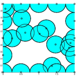
We consider a damaged wireless network presenting cover-age holes with a fixed boundary, in order to know the domain to cover, of which we can see an example in Figure 1.
We consider as inputs the set of existing vertices: the nodes of a damaged wireless network, and their coverage radii. Then an area is said to be covered when every points of the area
0 0.5 1 1.5 2 0 0.2 0.4 0.6 0.8 1 1.2 1.4 1.6 1.8 2
Fig. 1. A damaged wireless network with a fixed boundary.
are inside the covage disk of at least one vertex representing a network node. We also need a list of boundary nodes, these nodes can be fictional, but we need to know the whole area that is to be covered. We restrict ourselves to wireless networks with a fixed communication radius r, but it is possible to build the ˘Cech complex of a wireless network with different coverage radii using the intersection of different size coverage balls. The construction of the ˘Cech abstract simplicial complex for a fixed radius ris given:
Definition 1 ( ˘Cech complex): Given (X, d) a metric space whereX is a set and da distance,ω a finite set of N points in X, and r a real positive number. The ˘Cech complex of
ω, denoted Cr(ω), is the abstract simplicial complex whose k-simplices correspond to(k+ 1)-tuples of vertices inω for which the intersection of the k+ 1 balls of radiusrcentered at the k+ 1vertices is non-empty.
The ˘Cech complex characterizes the coverage of the wireless network. The k-th Betti numbers of an abstract simplicial complex X are defined as the number of k-th dimensional holes inX and are computed via linear algebra computations. For example, β0 counts the number of 0-dimensional holes,
that is the number of connected components. And β1 counts
the number of holes in the plane. Therefore the Betti number
β1of the ˘Cech complex counts the number of coverage holes
of the wireless network it represents.
The algorithm begins by adding new vertices in addition to the set of existing vertices presenting coverage holes. We suggest here the use of two common methods, and the new determinantal addition method. As we can see in Section IV, it is possible to consider deterministic or random based vertices addition methods: flexibility is one of the greatest advantage of our algorithm. In particular, it is possible to consider a method with pre-defined positions for some of the vertices in real-life scenarios.
For any undeterministic method, we choose that the number of added vertices, that we denote by Na, is determined as follows. First, it is set to be the minimum number of vertices needed to cover the whole area minus the number of existing vertices. This way, we take into account the number of existing vertices, that we denote by Ni. Then the Betti numbers β0 and β1 are computed via linear algebra thanks
to the simplicial complex representation. If there is still more than one connected component, and coverage holes, then the
number of added vertices Na is incremented with a random variableufollowing an exponential growth:
• Na:=da
2
πr2e −Ni,a2 being the area to cover.
• After adding theNa vertices, ifβ06= 1or β16= 0,
Then, Na=Na+u, andu= 2∗u.
The next step of our approach is to run the coverage reduction algorithm from [6] which maintains the topology of the wireless network: the algorithm removes vertices from the simplicial complex without modifying its Betti numbers. At this step, we remove some of the supernumerary vertices we just added in order to achieve an more efficient result with a minimum number of added vertices.
We give in Algorithm 1 the outline of the algorithm. The algorithm requires the set of initial vertices ωi, the fixed coverage radius r, as well as the list of boundary vertices
Lb. It is important to note that only connectivity information is needed to build the ˘Cech complex.
Algorithm 1 Disaster recovery algorithm
Require: Set of verticesωi, radius r, boundary verticesLb
Computation of the ˘Cech complexX =Cr(ωi) Na =da
2
πr2e −Ni
Addition ofNa vertices toX following chosen method Computation ofβ0(X)andβ1(X)
u= 1
while β06= 1or β16= 0 do
Na =Na+u u= 2∗u
Addition ofNavertices toXfollowing chosen method Computation ofβ0(X)andβ1(X)
end while
Coverage reduction algorithm on X
return ListLa of kept added vertices.
IV. VERTICES ADDITION METHODS
In this section, we propose two vertices addition methods. The aim of this part of the algorithm is to add enough vertices to patch the coverage of the simplicial complex, but the less vertices the better since the results will be closer to the optimal solution. We consider grid and uniform positioning as well as the use of the Sobol sequence, which require minimum simulation capacities and are well known in wireless networks management. The grid method is deterministic, so the number of added vertices as well as their position are set. The uniform and the Sobol methods are random, the number of added vertices is then computed as presented in Section III. A. Grid
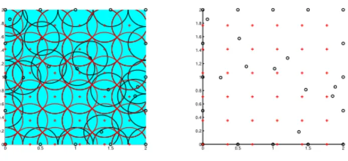
The first method we suggest ensures perfect coverage: the new vertices are positioned along a square grid in a lattice graph where the distance between two neighboring vertices is
√
2r. The number of vertices is set. Therefore this method is completely independent from the initial configuration. We can see an example of the grid vertices addition method on the
damaged network of Figure 1 in Figure 2. Existing vertices are black circles while added vertices are red plusses.
0 0.5 1 1.5 2 0 0.2 0.4 0.6 0.8 1 1.2 1.4 1.6 1.8 2 0 0.5 1 1.5 2 0 0.2 0.4 0.6 0.8 1 1.2 1.4 1.6 1.8 2
Fig. 2. With the grid addition method.
B. Uniform
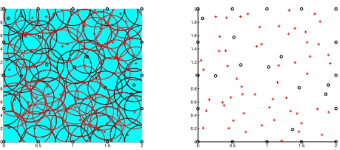
Here, the number of added vertices Na is computed ac-cordingly to the method presented in Section III, taking into account the number of existing vertices Ni. Then the Na vertices are sampled following a uniform law on the entire domain. An obtained configuration with this method on the network of Figure 1 is shown in Figure 3.
0 0.5 1 1.5 2 0 0.2 0.4 0.6 0.8 1 1.2 1.4 1.6 1.8 2 0 0.5 1 1.5 2 0 0.2 0.4 0.6 0.8 1 1.2 1.4 1.6 1.8 2
Fig. 3. With the uniform addition method.
C. Sobol sequence
Thanks to this method, we are able to take into account the positions of the new added vertices. The Sobol sequence is a statistical tool used to provide uniform coverage of the unit square. Thus, vertices positioned with the Sobol sequences reach complete coverage faster than uniform positioning be-cause the aggregation phenomenon is statistically avoided. The Sobol initialization set is known, for instance on a square the first position is the middle of the square, then come the middles of the four squares included in the big square, etc. To randomize the positions drawn, the points are scrambled. Therefore the complexity of the simulation of this method is really low.
For our simulation, we used the set of initialization numbers provided by Bratley and Fox in [20]. Then we scrambled the points produced with the random method described in [21]. An example of this method is given in Figure 4.
D. Comparison
We can compare the vertices addition method presented here along two variables: their complexity and their efficiency. First,
0 0.5 1 1.5 2 0 0.2 0.4 0.6 0.8 1 1.2 1.4 1.6 1.8 2 0 0.5 1 1.5 2 0 0.2 0.4 0.6 0.8 1 1.2 1.4 1.6 1.8 2
Fig. 4. With the Sobol sequence addition method.
we compare the complexities of the two methods. They all are of complexity O(Na): computations of Na positions for the first two methods, and the Sobol method scramble Na positions already known by most simulation tools. For the random methods we have to add the complexity of computing the coverage via the Betti numbers, which is of the order of the number of triangles times the number of edges that is
O((Na+Ni)5(ar)6)for a square of sideaaccording to [22]. To compare the methods efficiency we count the number of vertices each method adds on average to reach complete coverage. The grid method being determinist, the number of added vertices is constant: Na = (b√a2rc+ 1)2 for a
˘
Cech complex or Na = (b2arc+ 1)2 for a Vietoris-Rips complex which is an approximation of the ˘Cech complex easier to simulate. We can see in Table I the mean number of added vertices on 1000 simulations for each method in different scenarios on a square of side a = 1with coverage radiusr = 0.25, and a Vietoris-Rips complex. Scenarios are defined by the mean percentage of area covered before running the recovery algorithm: if there are many or few existing vertices, and thus few or many vertices to add. The damaged network is simulated by drawing nodes one by one uniformly, independently on the square the desired percentage of covered area is reached. Then the fixed boundary is added. We need to note that number of added vertices is computed following our incrementation method presented in Section III and these results only concern the vertices addition methods before the reduction algorithm runs.
% of area initially covered 20% 40% 60% 80% Grid method 9.00 9.00 9.00 9.00
Uniform method 32.51 29.34 24.64 15.63
Sobol sequence method 29.00 29.40 24.09 16.96
TABLE I
MEAN NUMBER OF ADDED VERTICESE[Na]
The grid method is the most efficient for the number of added vertices to cover the whole area, however it is not always practicable in a real life scenario where positions can not be defined with such precision, and any imprecision leads to a coverage hole. This method fares even or better both in complexity and in number of added vertices.
V. DETERMINANTAL ADDITION METHOD
In this section, we present the determinantal method and compare it to the two methods presented in Section IV. A. Definitions
The most common point process in wireless network repre-sentation is the Poisson point process. However in this process, conditionally to the number of vertices, their positions are independent from each other (as in the uniform positioning method presented in Section IV). This independence creates some aggregations of vertices, that is not convenient for our application. That is why we propose the use of processes creat-ing some repulsion between vertices. General point processes can be characterized by their so-called Papangelou intensity
c. Informally speaking, for xa location, and ω a realization of a given point process, that is a set of vertices, c(x, ω)
is the probability to have a vertex in an infinitesimal region around xknowing the set of verticesω. For Poisson process,
c(x, ω) = 1 for any x and any ω. A point process is said to be repulsive (resp. attractive) whenever c(x, ω) ≥ c(x, ζ)
(resp.c(x, ω)≤c(x, ζ)) as soon asω⊂ζ. For repulsive point processes, that means that the greater the set of vertices, the smaller the probability to have an other vertex.
There exists two types of repulsion models. The so-called hard-core processes create balls around vertices wherein the probability to draw another node is zero. But this approach has two drawbacks for our application. First, it is not easy to determine the size of the ball in which no other vertex can be drawn. If it is set to be the coverage disk, areas close to initially covered area may be hard to cover. Second, the simulation of an hard-core process with many vertices can be long to the hard rejection of vertices. Therefore, for our application, we choose the use of soft-core processes, where there is no area wherein no vertices can be drawn. Among soft-core repulsive point processes, we are in particular interested in determinantal processes:
Definition 2 (Determinantal point process): Given X a Polish space equipped with the Radon measure µ, and
K a measurable complex function on X2, we say that
N is a determinantal point process on X with kernel K
if it is a point process on X with correlation functions
ρn(x1, . . . , xn) = det(K(xi, xj)1≤i,j≤n) for every n ≥ 1 andx1, . . . , xn ∈X.
We can see that when two vertices xi and xj tends to be close to each other for i 6=j, the determinant tends to zero for any kernel K since two lines of the matrix tends to be the same. As a consequence, the correlation function tends to zero. That means that the vertices ofN repel each other. There exist as many determinantal point processes as functions K. We are interested in the following:
Definition 3 (Ginibre point process): The Ginibre point process is the determinantal point process with kernel
K(x, y) =P∞
k=1Bkφk(x)φk(y), whereBk, k= 1,2, . . ., are kindependent Bernoulli variables andφk(x) =√πk1 !e
−|x|2 2 xk for x∈Candk∈N.
The Ginibre point process is invariant with respect to trans-lations and rotations, making it relatively easy to simulate on a compact set. Moreover, the repulsion induced by a Ginibre point process is of electrostatic type. The repulsion is the same along every direction around vertices, creating circles of equal repulsion if there is only one vertex for example, and not lines of equal repulsion as can be seen with a Fourier basis instead of a Ginibre one. The principle behind the repulsion in the Ginibre point process can be seen in simulations via the probability density used to draw vertices positions. The probability to draw a vertex at the exact same position of an already drawn vertex is zero. Then, this probability increases, in a continuous way, with increasing distance from every existing vertices. Therefore the probability to draw a vertex is greater in areas the furthest away from every existing vertices, that is to say in coverage holes. Therefore, added vertices are almost automatically located in coverage holes thus reducing the number of superfluous vertices.
B. Simulation
Using determinantal point processes allows us to not only take into account the number of existing vertices, via the computation ofNa, but we also take into account the existing vertices positions, then every new vertex position as it is added. It suffices to consider theNi existing vertices as theNi first vertices sampled in the process, then each vertex is taken into account as it is drawn. The Ginibre process is usually defined on the whole plane thus we needed to construct a process with the same repulsive characteristics but which could be restricted to a compact set. Moreover, we needed to be able to set the number of vertices to draw. Due to space limitations, we will not delve into these technicalities but they are developed in [10]. We can see a realisation of our simulation for the recovery of the wireless network of Figure 1 in Figure 5.
0 0.5 1 1.5 2 0 0.2 0.4 0.6 0.8 1 1.2 1.4 1.6 1.8 2 0 0.5 1 1.5 2 0 0.2 0.4 0.6 0.8 1 1.2 1.4 1.6 1.8 2
Fig. 5. With the determinantal addition method with a Ginibre basis.
C. Comparison
We now compare the determinantal vertices addition method to the methods presented in Section IV.
As for the complexity, since the determinantal method takes into account the position of both existing vertices and randomly added vertices, it is the more complex. First taking into account the existing vertices positions is of complexity
O(N2
i), then the position drawing with the rejection sampling is of complexity O(Na(Na+Ni))at most. Thus we have a
final complexity ofO(Ni2+Na2+NaNi)). To which we add the Betti numbers computation complexity: O((Na+Ni)5(ra)6). We give in Table II the comparison between the mean num-ber of added vertices for the three methods. The simulation parameters being the same as Section IV. The determinantal method provides the best results in all scenarios among the random methods by far. And it is the best method among all for the almost covered scenario.
% of area initially covered 20% 40% 60% 80% Grid method 9.00 9.00 9.00 9.00
Uniform method 32.51 29.34 24.64 15.63
Sobol sequence method 29.00 29.40 24.09 16.96
Determinantal method 16.00 14.62 12.36 7.79
TABLE II
MEAN NUMBER OF ADDED VERTICESE[Na]
VI. REDUCTION ALGORITHM
In this section, we recall the steps of the reduction algorithm for simplicial complexes presented in [6]. The algorithm takes as input an abstract simplicial complex: here it is the ˘Cech complex of the wireless network plus the added vertices, and a list of boundary vertices. At this step we have ensured that we have one connected component β0= 1, and no coverage
holeβ1= 0, via the addition of a sufficient number of vertices.
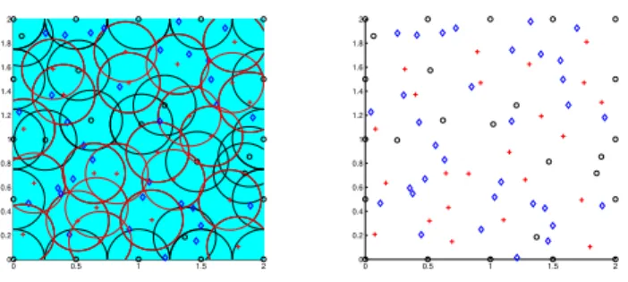
The first step is to characterize the superfluousness of 2 -simplices for the coverage with a degree defined to be the size of the largest simplex a2-simplex is the face of. Then to transmit the superfluousness of its 2-simplices to a vertex, an index of a vertex is defined to be the minimum of the degrees of the 2-simplices it is a face of. The indices give an order for an optimal removal of vertices: the greater the index of a vertex, the more likely it is superfluous for the coverage of its ˘Cech simplicial complex. In our disaster recovery case, we do not want to remove the remaining vertices of our damaged network. So these remaining vertices are given a negative index to flag them as unremovable, and only the newly added vertices are considered for removing. So, the vertices with the greatest index are candidates for removal: one is chosen randomly. If its removal does not change the homology, then it is effectively removed, otherwise it is flagged as unremovable with a negative index. The algorithm goes on until every remaining vertex is unremovable, thus achieving a unimprovable result. For more information on the reduction algorithm we refer to [6]. We can see in Figure 6 an execution of the reduction algorithm on the intermediate configuration of Figure 5. Removed vertices are represented by blue diamonds.
VII. PERFORMANCE COMPARISON
We now compare the performance results of the whole dis-aster recovery algorithm to the most known coverage recovery algorithm: the greedy algorithm for the set cover problem.
First, we compare their complexities. The greedy algorithm method lays a square grid of parameter √2r for the ˘Cech
0 0.5 1 1.5 2 0 0.2 0.4 0.6 0.8 1 1.2 1.4 1.6 1.8 2 0 0.5 1 1.5 2 0 0.2 0.4 0.6 0.8 1 1.2 1.4 1.6 1.8 2
Fig. 6. The reduction algorithm run on the determinantal method example.
complex of potential new vertices. Then the first added vertex is the furthest from all existing vertices. The algorithm goes on adding the furthest potential vertex of the grid from all vertices (existing+added). It stops when the furthest vertex is in the coverage ball of an existing or added vertex. Then for the
(i+ 1)-th vertex addition, the greedy algorithm computes the distances from allNi+iexisting vertices to all(b√a2rc+1)2−i potential vertices. Therefore the complexity of the greedy algorithm is inO((Ni+Na)(b√a2rc+1)2)). For the complexity of our algorithm, we consider first the complexity of building the simplicial complex associated with the network which is in O((Ni+Na)C), where C is the clique number. This complexity seems really high since C can only be upper bounded byNi+Na in the general case but it is the only way to compute the coverage when vertices position are not defined along a grid. Then the complexity of the coverage reduction algorithm is of the order ofO((1 + (ar)2)Ni+Na)(see [6]). So
the greedy algorithm appears less complex than ours in the general case. However whenris small before aor when the dimension is greater than 2, then the power factor becomes
d >2andC is a finite integer, so the trend is reversed. Then, we compare the mean number of added vertices in the final state. The final number of added vertices is the number of added vertices for the greedy algorithm, and the number of kept added vertices after the reduction for the homology algorithm. It is important to note that our algorithm with the grid method gives the exact same result as the greedy algorithm, number of added vertices and their positions being exactly the same. Results presented in Table III are simulated in the same conditions as in Section IV.
% of area initially covered 20% 40% 60% 80% Greedy algorithm 3.69 3.30 2.84 1.83
Homology algorithm 4.42 3.87 2.97 1.78
TABLE III
MEAN FINAL NUMBER OF ADDED VERTICESE
Nf
The numbers of vertices added in the final state both with our recovery algorithm and the greedy algorithm are roughly the same. They both tend to the minimum number of vertices required to cover the uncovered area depending on the initial configuration. Nonetheless, we can see that our algorithm performs a little bit worse than the greedy algorithm in the less
covered area scenarios because the vertices are not optimally positioned and it can be seen when just a small percentage of area is covered, and whole parts of the grid from the greedy algorithm are used, instead of isolated vertices. In compensation, our homology algorithm performs better in more covered scenarios.
To show the advantages of our homology based disaster recovery algorithm we choose to evaluate the robustness of the algorithm when the added vertices positions are slightly moved, i.e. when the nodes positioning does not strictly follow the theoretical positioning. In order to do this, we apply a Gaussian perturbation to each the added vertices position. The covariance matrix of the perturbation is given by Σ = σ2Id
with σ2 = 0.01, and where Id is the identity matrix of size the number of vertices. This means that the standard deviation for each vertex is of σ = 0.1. Other simulations parameters are unchanged, results in Table IV and V are given in mean over1000simulations. First, we compute the average number of holesβ1created by the Gaussian perturbation in Table IV.
Then in Table V, we counted the percentage of simulations in which the number of holes is still zero after the Gaussian perturbation on the new vertices positions.
% of area initially covered 20% 40% 60% 80% Greedy algorithm 0.68 0.65 0.45 0.35
Homology algorithm 0.62 0.53 0.37 0.26
TABLE IV
MEAN NUMBER OF HOLESE[β1]AFTER THEGAUSSIAN PERTURBATION
% of area initially covered 20% 40% 60% 80% Greedy algorithm 40.8% 47.7% 61.0% 69.3%
Homology algorithm 50.9% 58.1% 67.9% 75.3%
TABLE V
PROBABILITY THAT THERE IS NO HOLEP(β1= 0)AFTER THEGAUSSIAN
PERTURBATION
We can see that the perturbation on the number of holes decreases with the percentage of area initially covered, since the initial vertices are not perturbed. Our homology algorithm clearly performs better, even in the least covered scenarios, there are less than 50% of simulations that create coverage holes, which is not the case for the greedy algorithm. The greedy algorithm also always creates more coverage holes in mean than our disaster recovery algorithm for the same vertices positions perturbation. Therefore our algorithm seems more fitted to the disaster recovery case when a recovery network is deployed in emergency both indoor, via Femtocells, and outdoor, via a trailer fleet, where exact GPS locations are not always available, and exact theoretical positioning is not always followed.
VIII. CONCLUSION
In this paper, we adopt the simplicial homology represen-tation for wireless networks which characterizes not only the connectivity but also the coverage of a given network. Based
on that representation, we write an algorithm which patches coverage holes of damaged wireless networks by giving the positions in which to put new nodes. Our recovery algorithm first adds enough new nodes to cover the whole domain, then runs a reduction algorithm on the newly added nodes to reach a unimprovable result. The originality of the algorithm lies in the fact that we do not only add the needed nodes, thus providing a mathematically optimal but not reliable result, but adds too many nodes before removing the superfluous ones, thus providing a stronger coverage that is less sensitive to the imprecisions of following approximatively GPS locations. Moreover, the vertices addition methods can be chosen and adapted to a particular situation. In this paper we compared the use of classic positioning methods: grid, uniform and Sobol sequence, to the new determinantal method that is more efficient at positioning new vertices where they are needed.
REFERENCES
[1] Q. Fang, J. Gao, and L. Guibas, “Locating and bypassing routing holes in sensor networks,” inINFOCOM 2004. Twenty-third AnnualJoint Conference of the IEEE Computer and Communications Societies, vol. 4, march 2004, pp. 2458 – 2468 vol.4.
[2] C. Zhang, Y. Zhang, and Y. Fang, “Detecting coverage boundary nodes in wireless sensor networks,” inNetworking, Sensing and Control, 2006. ICNSC ’06. Proceedings of the 2006 IEEE International Conference on, 0-0 2006, pp. 868 –873.
[3] R. Ghrist and A. Muhammad, “Coverage and hole-detection in sensor networks via homology,” in Proceedings of the 4th international symposium on Information processing in sensor networks, ser. IPSN ’05. Piscataway, NJ, USA: IEEE Press, 2005. [Online]. Available: http://dl.acm.org/citation.cfm?id=1147685.1147729
[4] V. de Silva and R. Ghrist, “Coordinate-free coverage in sensor networks with controlled boundaries via homology,” International Journal of Robotics Research, vol. 25, december 2006.
[5] A. Muhammad and A. Jadbabaie, “Decentralized computation of homol-ogy groups in networks by gossip,” in American Control Conference, 2007. ACC ’07, july 2007, pp. 3438 –3443.
[6] A. Vergne, L. Decreusefond, and P. Martins, “Reduction algorithm for simplicial complexes,” inINFOCOM, 2013 Proceedings IEEE, 2013, pp. 475–479.
[7] N. Miyoshi and T. Shirai, “A cellular network model with ginibre configurated base stations,” Research Rep. on Math. and Comp. Sciences (Tokyo inst. of tech.), 2012. [Online]. Available: http://www.is.titech.ac.jp/research/research-report/B/B-467.pdf [8] G. L. Torrisi and E. Leonardi, “Large deviations of the interference in
the Ginibre network model,” arXiv:cs.IT/1304.2234,to appear, 2013. [9] N. Deng, W. Zhou, and M. Haenggi, “The ginibre point process as a
model for wireless networks with repulsion,” arXiv:cs.IT/1401.3677,to appear, Jan. 2014.
[10] L. Decreusefond, I. Flint, and A. Vergne, “Efficient simulation of the Ginibre process,” Oct. 2013, hal-00869259. [Online]. Available: http://hal.archives-ouvertes.fr/hal-00869259
[11] V. Chvatal, “A Greedy Heuristic for the Set-Covering Problem,”
Mathematics of Operations Research, vol. 4, no. 3, pp. 233–235, 1979. [Online]. Available: http://dx.doi.org/10.2307/3689577
[12] D. Haussler and E. Welzl, “Epsilon-nets and simplex range queries,” in Proceedings of the second annual symposium on Computational geometry, ser. SCG ’86. New York, NY, USA: ACM, 1986, pp. 61–71. [Online]. Available: http://doi.acm.org/10.1145/10515.10522 [13] Q. Fang, J. Gao, L. Guibas, V. de Silva, and L. Zhang, “GLIDER:
Gradient landmark-based distributed routing for sensor networks,” in
Proc. IEEE Conference on Computer Communications (INFOCOM), 2005.
[14] A.Nguyen, N.Milosavljevi´c, Q.Fang, J.Gao, and L.J.Guibas, “Landmark selection and greedy landmark-descent routing for sensor networks,” in
[15] C. Mueller, M. Kaschub, C. Blankenhorn, and S. Wanke, “A cell outage detection algorithm using neighbor cell list reports,” inSelf-Organizing Systems, ser. Lecture Notes in Computer Science. Springer Berlin Heidelberg, 2008, vol. 5343, pp. 218–229.
[16] M. Amirijoo, L. Jorguseski, T. Kurner, R. Litjens, M. Neuland, L. Schmelz, and U. Turke, “Cell outage management in LTE networks,” inWireless Communication Systems, 2009. ISWCS 2009. 6th Interna-tional Symposium on, 2009, pp. 600–604.
[17] 3GPP, “Telecommunications management; self-healing OAM; concepts and requirements,”Tech. Rep., vol. 3GPP TS 32.541 v1.6.1, 2010. [18] K. Morrison, “Rapidly recovering from the catastrophic loss of a major
telecommunications office,”Communications Magazine, IEEE, vol. 49, no. 1, pp. 28–35, 2011.
[19] A. Hatcher,Algebraic Topology. Cambridge University Press, 2002. [20] P. Bratley and B. L. Fox, “Algorithm 659: Implementing sobol’s
quasirandom sequence generator,” ACM Trans. Math. Softw., vol. 14, no. 1, pp. 88–100, Mar. 1988. [Online]. Available: http://doi.acm.org/10.1145/42288.214372
[21] J. Matoušek, “On the l2-discrepancy for anchored boxes,”J. Complex., vol. 14, no. 4, pp. 527–556, Dec. 1998. [Online]. Available: http://dx.doi.org/10.1006/jcom.1998.0489
[22] L. Decreusefond, E. Ferraz, H. Randriambololona, and A. Vergne, “Simplicial homology of random configurations,”Advances in Applied Probability, 2013.