Era of Big Data Processing: A New Approach via Tensor Networks and Tensor Decompositions

Era of Big Data Processing: A New Approach

via Tensor Networks and Tensor

Decompositions

Andrzej CICHOCKI

RIKEN Brain Science Institute, Japan

and Systems Research Institute of the Polish Academy of Science, Poland

[email protected]

Part of this work was presented on the International Workshop on Smart Info-Media Systems in Asia,

(invited talk - SISA-2013) Sept.30–Oct.2, 2013, Nagoya, Japan

Abstract—Many problems in computational neuroscience, neuroinformatics, pattern/image recognition, signal processing and machine learning generate massive amounts of multidimensional data with multiple aspects and high dimensionality. Tensors (i.e., multi-way arrays) provide often a natural and compact representation for such massive multidimensional data via suitable low-rank approximations. Big data analytics require novel technologies to efficiently process huge datasets within tolerable elapsed times. Such a new emerging technology for multidimensional big data is a multiway analysis via tensor networks (TNs) and tensor decompositions (TDs) which represent tensors by sets of factor (component) matrices and lower-order (core) tensors. Dynamic tensor analysis allows us to discover meaningful hidden structures of complex data and to perform generalizations by capturing multi-linear and multi-aspect relationships. We will discuss some fundamental TN models, their mathematical and graphical descriptions and associated learning algorithms for large-scale TDs and TNs, with many potential applications including: Anomaly detection, feature extraction, classification, cluster analysis, data fusion and integration, pattern recognition, predictive modeling, regression, time series analysis and multiway component analysis.

Keywords: Large-scale HOSVD, Tensor decompositions, CPD, Tucker models, Hierarchical Tucker (HT) decompo-sition, low-rank tensor approximations (LRA), Tensoriza-tion/Quantization, tensor train (TT/QTT) - Matrix Product States (MPS), Matrix Product Operator (MPO), DMRG, Strong Kronecker Product (SKP).

I. Introduction and Motivations

Big Data consists of multidimensional, multi-modal data-sets that are so huge and complex that they cannot be easily stored or processed by using standard comput-ers. Big data are characterized not only by big Volume but also another specific “V” features (see Fig. 1). High Volume implies the need for algorithms that are scalable; High Velocity address the challenges related to process data in near real-time, or virtually real-time; High Verac-ity demands robust and predictive algorithms for noisy, incomplete or inconsistent data, and finally, high Variety may require integration across different kind of data,

e.g., neuroimages, time series, spiking trains, genetic and behavior data. Many challenging problems for big data

PB TB GB MB VERACITY VOLUME VARIETY VELOCITY Batch Genetic Expressions, Behaviour Data Micro-batch Periodic Near Real Time

Real Time

EEG,MEG,EMG Spectrogram

s

Time SeriesECoG,MRI,MUR

Neuroimage,_{Spikes fMRI+DTI+PET} Anomaly

Inconsitent Biased_{Incomplete Data} Noise

Figure 1:Big Data analysis for neuroscience recordings. Brain data can be recorded by electroencephalography (EEG), electro-corticography (ECoG), magnetoencephalography (MEG), fMRI, DTI, PET, Multi Unit Recording (MUR). This involves analysis of multiple modalities/multiple subjects neuroimages, spec-trograms, time series, genetic and behavior data. One of the challenges in computational and system neuroscience is to make fusion (assimilation) of such data and to understand the multiple relationships among them in such tasks as perception, cognition and social interactions. The our “V”s of big data: Volume scale of data, Variety different forms of data, Veracity -uncertainty of data, and Velocity - analysis of streaming data, comprise the challenges ahead of us.

are related to capture, manage, search, visualize, cluster, classify, assimilate, merge, and process the data within a tolerable elapsed time, hence demanding new innovative solutions and technologies. Such emerging technology is Tensor Decompositions (TDs) and Tensor Networks (TNs) via low-rank matrix/tensor approximations. The challenge is how to analyze large-scale, multiway data

Figure 2:A 3rd-order tensorX∈RI×J×K_{, with entriesx} i,j,k= X(i,j,k) and its sub-tensors: Slices and fibers. All fibers are treated as column vectors.

sets. Data explosion creates deep research challenges that require new scalable, TD and TN algorithms.

Tensors are adopted in diverse branches of science such as a data analysis, signal and image processing [1]–[4], Psychometric, Chemometrics, Biometric, Quan-tum Physics/Information, and QuanQuan-tum Chemistry [5]– [7]. Modern scientific areas such as bioinformatics or computational neuroscience generate massive amounts of data collected in various forms of large-scale, sparse tabular, graphs or networks with multiple aspects and high dimensionality.

Tensors, which are multi-dimensional generalizations of matrices (see Fig. 2 and Fig. 3), provide often a useful representation for such data. Tensor decompo-sitions (TDs) decompose data tensors in factor matri-ces, while tensor networks (TNs) represent higher-order tensors by interconnected lower-order tensors. We show that TDs and TNs provide natural extensions of blind source separation (BSS) and 2-way (matrix) Component Analysis (2-way CA) to multi-way component analysis (MWCA) methods. In addition, TD and TN algorithms are suitable for dimensionality reduction and they can handle missing values, and noisy data. Moreover, they are potentially useful for analysis of linked (coupled)

(a) G G . . . G₁₁ G₁₂ G₁ K Û ... (b)

Û

...

Figure 3:Block matrices and their representations by (a) a 3rd-order tensor and (b) a 4th-3rd-order tensor.

block of tensors with millions and even billions of non-zero entries, using the map-reduce paradigm, as well as divide-and-conquer approaches [8]–[10]. This all sug-gest that multidimensional data can be represented by linked multi-block tensors which can be decomposed into common (or correlated) and distinctive (uncorre-lated) components [3], [11], [12]. Effective analysis of coupled tensors requires the development of new models and associated algorithms that can identify the core relations that exist among the different tensor modes, and the same tome scale to extremely large datasets. Our objective is to develop suitable models and algo-rithms for linked low-rank tensor approximations (TAs), and associated scalable software to make such analysis possible.

Review and tutorial papers [2], [4], [13]–[15] and books [1], [5], [6] dealing with TDs already exist, however, they typically focus on standard TDs and/or do not provide explicit links to big data processing topics and do not explore natural connections with emerging areas including multi-block coupled tensor analysis and tensor networks. This paper extends beyond the standard TD models and aims to elucidate the power and flexibility of TNs in the analysis of multi-dimensional, multi-modal, and multi-block data, together with their role as a math-ematical backbone for the discovery of hidden structures in large-scale data [1], [2], [4].

Motivations - Why low-rank tensor approximations?

A wealth of literature on (2-way) component analysis (CA) and BSS exists, especially on Principal Compo-nent Analysis (PCA), Independent CompoCompo-nent Analysis (ICA), Sparse Component Analysis (SCA), Nonnegative Matrix Factorizations (NMF), and Morphological Com-ponent Analysis (MCA) [1], [16], [17]. These techniques are maturing, and are promising tools for blind source separation (BSS), dimensionality reduction, feature ex-traction, clustering, classification, and visualization [1], [17].

Figure 4:Basic symbols for tensor network diagrams.

The “flattened view” provided by 2-way CA and matrix factorizations (PCA/SVD, NMF, SCA, MCA) may be inappropriate for large classes of real-world data which exhibit multiple couplings and cross-correlations. In this context, higher-order tensor networks give us the opportunity to develop more sophisticated models per-forming distributed computing and capturing multiple interactions and couplings, instead of standard pairwise interactions. In other words, to discover hidden com-ponents within multiway data the analysis tools should account for intrinsic multi-dimensional distributed pat-terns present in the data.

II. Basic Tensor Operations

A higher-order tensor can be interpreted as a multiway array, as illustrated graphically in Figs. 2, 3 and 4. Our adopted convenience is that tensors are denoted by bold underlined capital letters, e.g., X ∈ RI₁×I2×···×IN_{, and} that all data are real-valued. The order of a tensor is the number of its “modes”, “ways” or “dimensions”, which can include space, time, frequency, trials, classes, and dictionaries. Matrices (2nd-order tensors) are denoted by boldface capital letters, e.g., X, and vectors (1st-order tensors) by boldface lowercase letters; for instance the columns of the matrix A = [a1,a2, . . . ,aR] ∈ RI×R are

denoted by ar and elements of a matrix (scalars) are

denoted by lowercase letters, e.g., air (see Table I).

The most common types of tensor multiplications are denoted by: ⊗ for the Kronecker, for the Khatri-Rao, ~ for the Hadamard (componentwise), ◦ for the outer and ×n for the mode-n products (see Table II).

TNs and TDs can be represented by tensor network diagrams, in which tensors are represented graphically by nodes or any shapes (e.g., circles, spheres, triangular, squares, ellipses) and each outgoing edge (line) emerging from a shape represents a mode (a way, dimension, indices) (see Fig. 4) Tensor network diagrams are very useful not only in visualizing tensor decompositions, but also in their different transformations/reshapings and graphical illustrations of mathematical (multilinear) operations.

It should also be noted that block matrices and hier-archical block matrices can be represented by tensors.

TABLE I:Basic tensor notation and symbols. A tensor are de-noted by underline bold capital letters, matrices by uppercase bold letters, vectors by lowercase boldface letters and scalars by lowercase letters.

X∈RI1×I2×···×IN _{Nth-order tensor of size}

I1×I2× · · · ×IN G, Gr, GX, GY, S core tensors

Λ∈RR×R×···×R Nth-order diagonal core

ten-sor with nonzero λr entries on

main diagonal

A= [a1,a2, . . . ,aR]∈RI×R matrix with column vectors ar∈RI _{and entriesa} ir A,B,C, B(n), U(n) component matrices i= [i1,i2, . . . ,iN] vector of indices X_(n)∈RIn×I1···In−1In+1···IN mode-nunfolding ofX

x:,i2,i3,...,iN mode-1 fiber of X obtained by fixing all but one index X:,:,i3,...,iN tensor slice of X obtained by

fixing all but two indices

X:,:,:,i4,...,iN subtensor of X, in which sev-eral indices are fixed

x=vec(X) vectorization ofX

diag{•} diagonal matrix

For example, 3rd-order and 4th-order tensors that can be represented by block matrices as illustrated in Fig. 3 and all algebraic operations can be performed on block matrices. Analogously, higher-order tensors can be rep-resented as illustrated in Fig. 5 and Fig. 6. Subtensors are formed when a subset of indices is fixed. Of particular interest are fibers, defined by fixing every index but one, andmatrix sliceswhich are two-dimensional sections (matrices) of a tensor, obtained by fixing all the indices but two (see Fig. 2). A matrix has two modes: rows and columns, while an Nth-order tensor has Nmodes.

The process of unfolding (see Fig. 7) flattens a ten-sor into a matrix. In the simplest scenario, mode-n

unfolding (matricization, flattening) of the tensor A ∈ RI1×I2×···×IN _{yields a matrixA}

(n)∈RIn×(I1···In−1In+1···IN), with entries ain,(j1,...,in−1,jn+1,...,in) such that remaining in-dices(i1, . . . ,in−1,in+1, . . . ,iN)are arranged in a specific

order, e.g., in the lexicographical order [4]. In tensor networks we use, typically a generalized mode-([n])

unfolding as illustrated in Fig. 7 (b).

By a multi-index i = i1,i2, . . . ,iN, we denote an

index which takes all possible combinations of values of i1,i2, . . . ,in, for in = 1, 2, . . . ,In in a specific and

consistent orders. The entries of matrices or tensors in matricized and/or vectorized forms can be ordered in

(a) X X R1 1I R2 2I I1 I2 R1 R2 1 2 (I ´I ) (b)

...

Vector (each entry is a block matrix)

Block matrix

Matrix

(c)

Matrix

=

Figure 5: Hierarchical block matrices and their representa-tions as tensors: (a) a 4th-order tensor for a block matrix X∈RR1I1×R2I2_{, comprising block matrices X}

r1,r2 ∈ R

I1×I2_{, (b)}

a 5th-order tensor and (c) a 6th-order tensor.

at least two different ways.

Remark: The multi–index can be defined using two

different conventions:

1) The little-endian convention

i1,i2, . . . ,iN = i1+ (i2−1)I1+ (i3−1)I1I2 · · · +(iN−1)I1· · ·IN−1. (1) 2) The big-endian

i1,i2, . . . ,iN=iN+ (iN−1−1)IN+

+(iN−2−1)ININ−1+· · ·+ (i1−1)I2· · ·IN. (2)

The little–endian notation is consistent with the For-tran style of indexing, while the big–endian notation is similar to numbers written in the positional system and corresponds to reverse lexicographic order. The def-inition unfolding of tensors and the Kronecker (tensor) product ⊗ should be also consistent with the chosen

. . . = 4th-order tensor = 5th-order tensors = 6th-order tensor

Figure 6: Graphical representations and symbols for higher-order block tensors. Each block represents a 3rd-higher-order tensor or 2nd-order tensor. An external circle represent a global structure of the block tensor (e.g., a vector, a matrix, a 3rd-order tensor) and inner circle represents a structure of each element of the block tensor.

convention1. In this paper we will use the big-endian no-tation, however it is enough to remember thatc=a⊗b means thatc_i,j =aibj.

The Kronecker product of two tensors: A ∈ RI1×I2···×IN _{and B ∈} RJ1×J2×···×JN _{yields C = A⊗B ∈} RI1I2×···×INJN_{, with entries c}

i1,j1,...,iN,jN = ai1,...,iNbj1,...,jN, wherein,jn =jn+ (in−1)Jn.

The mode-n product of a tensor A ∈ RI1×···×IN _by a vector b ∈ RIn _{is defined as a tensor C = A×}¯_{nb ∈} RI1×···×In−1×In+1×···×IN_{, with entries ci}

1,...,in−1,in+1,...,iN =

∑In

in=1(ai1,i2,...,iN) bin, while a mode-n product of the tensor A ∈ RI1×···×IN _{by a matrix B ∈} RJ×In _{is the} tensor C = A×nB ∈ RI1×···×In−1×J×In+1×···×IN, with

entriesci1,i2,...,in−1,j,in+1,...,iN =∑

In

in=1ai1,i2,...,iN bj,in. This can also be expressed in a matrix form as C(n)=BA(n) (see Fig. 8), which allows us to employ fast matrix by vector and matrix by matrix multiplications for very large scale problems.

If we take all the modes, then we have a full multilin-ear product of a tensor and a set of matrices, which is compactly written as [4] (see Fig. 9 (a))):

C = G×1B(1)×2B(2)· · · ×NB(N)

= JG;B(1),B(2), . . . ,B(N)K. (3)

In a similar way to mode-n multilinear prod-uct, we can define the mode-(m_n) product of two tensors (tensor contraction) A ∈ RI1×I2×...×IN _and

1_{The standard and more popular definition in multilinear algebra}

assumes the big–endian convention, while for the development of the efficient program code for big data usually the little–endian convention seems to be more convenient (see for more detail papers of Dolgov and Savostyanov [18], [19]).

(a) (b)

A

I

_I

I

I

I

_I

I

I

I

I

I

J

Þ

_...

A

. .. ...

...

A

=

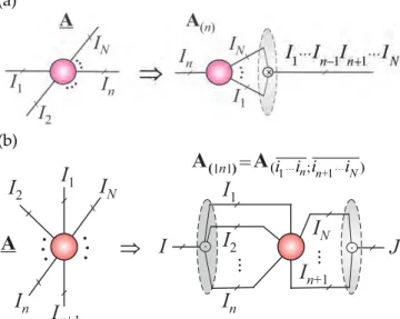
Figure 7: Unfoldings in tensor networks: (a) Graphical rep-resentation of the basic mode-nunfolding (matricization, flat-tening) A(n)∈RIn×I1···In−1In+1···IN for anNth-order tensorA∈ RI1×I2×···×IN_{. (b) More general unfolding of theNth-order} ten-sor into a matrixA([n])=A(i1,...,in;in+1,...,iN)∈R

I1I2···In×In+1···IN_. All entries of an unfolded tensor are arranged in a specific order, e.g., in lexicographical order. In a more general case, let r = {m1,m2, . . . ,mR} ⊂ {1, 2, . . . ,N} be the row indices

and c = {n1,n2, . . . ,nC} ⊂ {1, 2, . . . ,N} −r be the column

indices, then the mode-(r,c) unfolding of A is denoted as A_(r,c)∈RIm₁Im2···ImR×In₁In2···InC_. (a) ... ... ... ... A C B B A(1) C(1) I2 I1 I3 I2 I1 J J J J I1 2 3 I I× I1

Û

Figure 8: From a matrix format to the tensor network for-mat. (a) Multilinear mode-1 product of a 3rd-order tensor A ∈ RI1×I2×I3 _{and a factor (component) matrix B ∈} RJ×I1

yields a tensor C = A×₁B ∈ RJ×I2×I3_{. This is equivalent}

to simple matrix multiplication formula C₍₁₎ = BA₍₁₎. (b) Multilinear mode-n product anNth-order tensor and a factor matrixB∈RJ×In_.

B ∈ RJ1×J2×···×JM_{, with common modes In =}

Jm that yields an (N + M −2)-order tensor C ∈

RI1×···In−1×In+1×···×IN×J1×···Jm−1×Jm+1×···×JM_:

C=A×m_n B, (4)

with entries ci₁,...i_n−1,in+1,...iN,j1,...jm−1,jm+1,...jM =

TABLE II: Basic tensor/matrix operations.

C=A×nB mode-n product ofA ∈RI1×I2×···×IN and B ∈ RJn×In _yields C ∈ RI1×···×In−1×Jn×In+1×···×IN_, with entries ci1,...,in−1,j,in+1,...iN = ∑In in=1ai1,...,in,...,iNbj,in, or equivalently C_(n) =B A_(n) C=_JA;B(1), . . . ,B(N)K=A×1B (1)_× 2B(2)· · · ×NB(N)

C=A◦B tensor or outer product of A

∈ RI1×I2×···×IN _{and B ∈} RJ1×J2×···×JM yields(N+M)th-order tensorC, with entriesci1,...,iN,j1,...,jM=ai1,...,iNbj1,...,jM

X=a◦b◦c∈RI×J×K tensor or outer product of vectors

forms a rank-1 tensor, with entries xijk=aibjck

AT, A−1,A† transpose, inverse and Moore-Penrose pseudo-inverse ofA

C=A⊗B

Kronecker product of A ∈ RI1×I2×···×IN _{and B ∈} RJ1×J2×···×JN yieldsC∈RI1J1×···×INJN_{, with entries}

c_i 1,j1,...,iN,jN = ai1,...,iN bj1,...,jN, where in,jn=jn+ (in−1)Jn C=AB Khatri-Rao product ofA∈R I×J _and B ∈ RK×J _{yields C ∈ R}IK×J_{, with} columnsc_j=a_j⊗b_j ∑In i=1ai1,...in−1,i in+1,...iNbj1,...jm−1,i,jm+1,...jM (see Fig. 10 (a)). This operation can be considered as a contraction of two tensors in single common mode. Tensors can be contracted in several modes or even in all modes as illustrated in Fig. 10.

If not confusing a super- or sub-index m,n can be neglected. For example, the multilinear product of the tensors A∈ RI1×I2×···×IN _{and B∈} RJ1×J2×···×JM_{, with a} common modes IN= J1 can be written as

C=A ×1 N B=A×NB=A•B ∈ RI1×I2××IN−1××J2×···×JM_{, (5)} with entries: ci2,i3,...,iN,j1,j3,...,jM = ∑ I1 i=1ai,i2,...,iN bj1,i,j3,...,jM. Furthermore, note that for multiplications of matrices and vectors this notation implies that A×1

2B = AB, A×2 2B = ABT, A× 1,2 1,2B = hA,Bi, and A×12x = A×₂x=Ax.

Remark: If we use contraction for more than two

tensors the order has to be specified (defined) as follows:

A×b

aB×dcC=A×ba(B×dcC)forb<c.

The outer or tensor product C = A◦B of the ten-sors A ∈ RI1×···×IN _{and B ∈} RJ1×···×JM _{is the tensor}

C ∈ RI1×···×IN×J1×···×JM_{, with entries ci}

1,...,iN,j1,...,jM =

(a) (b)

R

R

R

B

R

B

B

B

B

I

I

I

I

I

R

G

I

I

I

I

A

_b

b

b

Figure 9: Multilinear products via tensor network diagrams. (a) Multilinear full product of tensor (Tucker decomposition) G ∈ RR1×R2×···×R5 _{and factor (component) matrices B}(n) _∈ RIn×Rn_{(n=1, 2, . . . , 5) yields the Tucker tensor decomposition} C=G×₁B(1)_×

2B(2)· · · ×5B(5)∈RI1×I2×···×I5. b) Multilinear product of tensor A∈RI1×I2×···×I4_{and vectors bn∈}RIn _(n= 1, 2, 3)yields a vectorc=Aׯ₁b(1)ׯ₂b(2)ׯ₃b(3)∈RI4_. I 1 I 2 J3 J 4 A B I J 4=1 I J 3=2 I 4=J2 I_N J₂ J1 J_m +1 J M A I J _B n

=

...

_...

...

_{. . .}

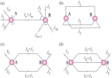
Figure 10: Examples of tensor contractions: (a) Multilinear product of two tensors is denoted by C=A ×m

n B. (b) Inner

product of two 3rd-order tensors yields a scalar c=hA,Bi=

A ×1,2,3_1,2,3 B = A × B = _∑i1,i2,i3 ai1,i2,i3 bi1,i2,i3. (c) Tensor

contraction of two 4th-order tensors yields C =A ×1,2_4,3 B ∈ RI1×I2×J3×J4_{, with entries c}

i1,i2,j3,j4 = ∑i3,i4 ai1,i2,i3,i4 bi4,i3,j3,j4.

(d) Tensor contraction of two 5th-order tensors yields 4th-order tensor C = A ×1,2,3_3,4,5 B ∈ RI1×I2×J4×J5_{, with entries}

ci1,i2,j4,j5=∑i3,i4,i5 ai1,i2,i3,i4,i5bi5,i4,i3,j4,j5.

nonzero vectors a ∈ RI_{, b ∈ R}J _{produces a}

rank-1 matrix X = a◦b = abT ∈ RI×J _{and the outer}

product of three nonzero vectors: a ∈ RI_{, b ∈ R}J

and c ∈ RK _{produces a 3rd-order rank-1 tensor: X =}

a◦b◦c ∈ RI×J×K_{, whose entries are x}

ijk = ai bj ck. A

tensor X∈RI₁×I2×···×IN _{is said to be rank-1 if it can be} expressed exactly as X= b1◦b2◦ · · · ◦bN, with entries xi1,i2,...,iN = bi1bi2· · ·biN, where bn ∈ R

In _{are nonzero} vectors. We refer to [1], [4] for more detail regarding the basic notations and tensor operations.

Z ] I1I₂I 3I4 I5 I6 X _® I1 I2 I3 I4 I5 I6 I7I8I9 I7 I8 I9 TT=MPS PEPS HT I1 I2 I3I4 I5I6 I7 I8 I9 I1 I2 I3 I4 I5 I6 I7 I8 I9

Figure 11: Examples of tensor networks. Illustration of rep-resentation of 9th-order tensor X ∈ RI1×I2×···×I9 _by

dif-ferent kinds of tensor networks (TNs): Tensor Train (TT) which is equivalent to the Matrix Product State (MPS) (with open boundary conditions (OBC)), the Projected Entangled-Pair State (PEPS), called also Tensor Product States (TPS, and Hierarchical Tucker (HT) decomposition, which is equivalent to the Tree-Tensor Network State (TTNS). The objective is to decompose a high-order tensor into sparsely connected low-order and low-rank tensors, typically 3rd-low-order and/or 4th-order tensors, called cores.

III. Tensor Networks

A tensor network aims to represent or decompose a higher-order tensor into a set of lower-order tensors (typically, 2nd (matrices) and 3rd-order tensors called cores or components) which are sparsely interconnected. In other words, in contrast to TDs, TNs represent de-compositions of the data tensors into a set of sparsely (weakly) interconnected lower-order tensors. Recently, the curse of dimensionality for higher-order tensors has been considerably alleviated or even completely avoided through the concept of tensor networks (TN) [20], [21]. A TN can be represented by a set of nodes interconnected by lines. The lines (leads, branches, edges) connecting tensors between each other correspond to contracted modes, whereas lines that do not go from one tensor to another correspond to open (physical) modes in the TN (see Fig. 11).

An edge connecting two nodes indicates a contraction of the respective tensors in the associated pair of modes as illustrated in Fig. 10. Each free (dangling) edge cor-responds to a mode, that is not contracted and, hence, the order of the entire tensor network is given by the number of free edges (called often physical indices). A tensor network may not contain any loops, i.e., any edges connecting a node with itself. Some examples of tensor network diagrams are given in Fig. 11.

If a tensor network is a tree, i.e., it does not contain any cycle, each of its edges splits the modes of the data tensor into two groups, which is related to the suitable matri-cization of the tensor. If, in such a tree tensor network, all nodes have degree 3 or less, it corresponds to an Hierarchical Tucker (HT) decomposition shown in Fig. 12 (a). The HT decomposition has been first introduced

in scientific computing by Hackbusch and K ¨uhn and further developed by Grasedyck, Kressner, Tobler and others [7], [22]–[26]. Note that for 6th-order tensor, there are two such tensor networks (see Fig. 12 (b)), and for 10th-order there are 11 possible HT decompositions [24], [25].

A simple approach to reduce the size of core tensors is to apply distributed tensor networks (DTNs), which consists in two kinds of cores (nodes): Internal cores (nodes) which have no free edges and external cores which have free edges representing physical indices of a data tensor as illustrated in Figs. 12 and 13.

The idea in the case of the Tucker model, is that a core tensor is replaced by distributed sparsely interconnected cores of lower-order, resulting in a Hierarchical Tucker (HT) network in which only some cores are connected (associated) directly with factor matrices [7], [22], [23], [26].

For some very high-order data tensors it has been observed that the ranksRn(internal dimensions of cores)

increase rapidly with the order of the tensor and/or with an increasing accuracy of approximation for any choice of tensor network, that is, a tree (including TT and HT decompositions) [25]. For such cases, the Pro-jected Entangled-Pair State (PEPS) or the Multi-scale Entanglement Renormalization Ansatz (MERA) tensor networks can be used. These contain cycles, but have hierarchical structures (see Fig. 13). For the PEPS and MERA TNs the ranks can be kept considerably smaller, at the cost of employing 5th and 4th-order cores and consequently a higher computational complexity w.r.t. tensor contractions. The main advantage of PEPS and MERA is that the size of each core tensor in the internal tensor network structure is usually much smaller than the cores in TT/HT decompositions, so consequently the total number of parameters can be reduced. However, it should be noted that the contraction of the resulting tensor network becomes more difficult when compared to the basic tree structures represented by TT and HT models. This is due to the fact that the PEPS and MERA tensor networks contain loops.

IV. Basic Tensor Decompositions and their

Representation via Tensor Networks Diagrams

The main objective of a standard tensor decomposition is to factorize a data tensor into physically interpretable or meaningful factor matrices and a single core tensor which indicates the links between components (vectors of factor matrices) in different modes.

A. Constrained Matrix Factorizations and

Decomposi-tions – Two-Way Component Analysis

Two-way Component Analysis (2-way CA) exploitsa

prioriknowledge about different characteristics, features

or morphology of components (or source signals) [1], [27] to find the hidden components thorough constrained

(a) (b)

Order 3:

Order 4:

Order 5:

Order 6:

Order 7:

Order 8:

Figure 12: (a) The standard Tucker decomposition and its transformation into Hierarchical Tucker (HT) model for an 8th-order tensor using interconnected 3rd-8th-order core tensors. (b) Various exemplary structure HT/TT models for different order of data tensors. Green circles indicate factor matrices while red circles indicate cores.

I8 I1 I2 I3 I4 I5 I6 I7 Þ I1 I2 I3 I4 I5 I6 I7 I8

Figure 13: Alternative distributed representation of 8th-order Tucker decomposition where a core tensor is replaced by MERA (Multi-scale Entanglement Renormalization Ansatz) tensor network which employs 3rd-order and 4th-order core tensors. For some data-sets, the advantage of such model is relatively low size (dimensions) of the distributed cores.

matrix factorizations of the form

X=ABT+E= R

∑

∑

where the constraints imposed on factor matrices A

and/orBinclude orthogonality, sparsity, statistical inde-pendence, nonnegativity or smoothness. The CA can be considered as a bilinear (2-way) factorization, whereX∈ RI×J _{is a known matrix of observed data,E∈R}I×J

rep-resents residuals or noise, A = [a1,a2, . . . ,aR] ∈ RI×R

is the unknown (usually, full column rank R) mixing matrix with R basis vectors ar ∈ RI, and B = [b1,b2, . . . ,bR] ∈ RJ×R is the matrix of unknown components

(factors, latent variables, sources).

Two-way component analysis (CA) refers to a class of signal processing techniques that decompose or en-code superimposed or mixed signals into components with certain constraints or properties. The CA meth-ods exploit a priori knowledge about the true nature or diversities of latent variables. By diversity, we refer to different characteristics, features or morphology of sources or hidden latent variables [27].

For example, the columns of the matrix B that rep-resent different data sources should be: as statistically independent as possible for ICA; as sparse as possible for SCA; take only nonnegative values for (NMF) [1], [16], [27].

Remark: Note that matrix factorizations have an

in-herent symmetry, Eq. (6) could be written asXT≈BAT, thus interchanging the roles of sources and mixing pro-cess.

Singular value decomposition (SVD) of the data matrix

X∈RI×J _{is a special case of the factorization in Eq. (6).}

It is exact and provides an explicit notion of the range and null space of the matrix X (key issues in low-rank approximation), and is given by

X=UΣVT= R

∑

∑

where Uand Vare column-wise orthonormal matrices and Σis a diagonal matrix containing only nonnegative singular values σr.

Another virtue of component analysis comes from a representation of multiple-subject, multiple-task datasets by a set of data matrices Xk, allowing us to perform

simultaneous matrix factorizations:

Xk ≈AkBTk, (k=1, 2, . . . ,K), (8)

subject to various constraints. In the case of statistical independence constraints, the problem can be related to models of group ICA through suitable pre-processing, dimensionality reduction and post-processing proce-dures [28].

The field of CA is maturing and has generated efficient algorithms for 2-way component analysis (especially, for sparse/functional PCA/SVD, ICA, NMF and SCA) [1], [16], [29]. The rapidly emerging field of tensor de-compositions is the next important step that naturally generalizes 2-way CA/BSS algorithms and paradigms. We proceed to show how constrained matrix factor-izations and component analysis (CA) models can be naturally generalized to multilinear models using con-strained tensor decompositions, such as the Canonical Polyadic Decomposition (CPD) and Tucker models, as illustrated in Figs. 14 and 15.

B. The Canonical Polyadic Decomposition (CPD)

The CPD (called also PARAFAC or CANDECOMP) factorizes an Nth-order tensor X ∈ RI1×I2×···×IN _{into a} linear combination of termsbr(1)◦br(2)◦ · · · ◦b(rN), which

are rank-1 tensors, and is given by [30]–[32]

X∼= R

∑

where the only non-zero entries λr of the diagonal

core tensor G = Λ ∈ RR×R×···×R _{are located on the}

main diagonal (see Fig. 14 for a 3rd-order and 4th-order tensors).

Via the Khatri-Rao products the CPD can also be expressed in a matrix/vector form as:

X(n)∼=B(n)Λ(B(1) · · · B(n−1)B(n+1) · · · B(N))T vec(X)∼= [B(1)B(2) · · · B(N)]λ, (10) where B(n) = [b(₁n),b₂(n), . . . ,b(_Rn)] ∈ RIn×R_{, λ =}

[λ1,λ2, . . . ,λR]T andΛ=diag{λ}is a diagonal matrix.

The rank of tensorX is defined as the smallest R for which CPD (9) holds exactly.

Algorithms to compute CPD.In the presence of noise

in real world applications the CPD is rarely exact and has to be estimated by minimizing a suitable cost function, typically of the Least-Squares (LS) type in the form of the Frobenius norm ||X−JΛ;B

(1)_,B(2)_{, . . . ,B}(N) K||F,

or using Least Absolute Error (LAE) criteria [33]. The Alternating Least Squares (ALS) algorithms [1], [13],

(a) Standard block diagram @ X B(1) J I K = K GC = +. . .+ (I R´ ) (R R R´ ´ ) (R J´ ) (R R K´ ´ ) (I R´ ) (R J´ ) 1 λ λ_R B(3)_Λ

Λ

(b) CPD in tensor network notation

I

I

I

I

X

=

I

I

I

I

R R

R

R

B

B

B

B

Λ

~

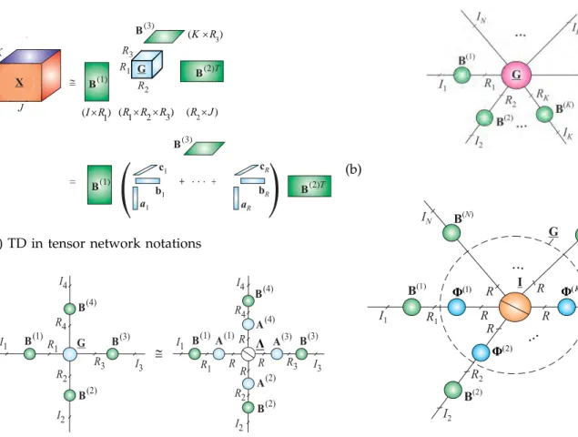
Figure 14: Representation of the CPD. (a) The Canonical Polyadic Decomposition (CPD) of a 3rd-order tensor as: X∼=

Λ×₁B(1)_×

2B(2)×3B(3) = ∑Rr=1λr b

(1)

r ◦b(r2)◦br(3) =Gc×1 B(1)×2B(2)withG=ΛandGc=Λ×3B(3). (b) The CPD for a 4th-order tensor as:X∼=Λ×₁B(1)×₂B(2)×₃B(3)×₄B(4)=

∑R r=1b

(1)

r ◦b(r2)◦br(3)◦b(r4). The objective of the CPD is to

estimate the factor matrices B(n) and a rank of tensor R, that is, the number of components R.

[31], [34] minimize the LS cost function by optimizing individually each component matrix, while keeping the other component matrices fixed. For instance, assume that the diagonal matrix Λ has been absorbed in one of the component matrices; then, by taking advantage of the Khatri-Rao structure the component matricesB(n)

can be updated sequentially as [4]

B(n)←X_(n)   K k6=n B(k)   ~k6=n(B(k)TB(k)) † , (11) which requires the computation of the pseudo-inverse of small (R×R)matrices.

The ALS is attractive for its simplicity and for well defined problems (not too many, well separated, not

collinear components) and high SNR, the performance of ALS algorithms is often satisfactory. For ill-conditioned problems, more advanced algorithms exist, which typ-ically exploit the rank-1 structure of the terms within CPD to perform efficient computation and storage of the Jacobian and Hessian of the cost function [35], [36].

Constraints. The CPD is usually unique by itself,

and does not require constraints to impose uniqueness [37]. However, if components in one or more modes are known to be e.g., nonnegative, orthogonal, statis-tically independent or sparse, these constraints should be incorporated to relax uniqueness conditions. More importantly, constraints may increase the accuracy and stability of the CPD algorithms and facilitate better physical interpretability of components [38], [39].

C. The Tucker Decomposition

The Tucker decomposition can be expressed as follows [40]: X ∼= R1

∑

∑

where X ∈ RI1×I2×···×IN _{is the given data tensor,}

G ∈ RR1×R2×···×RN _{is the core tensor and B}(n) ₌

[b(₁n),b(₂n), . . . ,b_R(n_n)]∈RIn×Rn _{are the mode-ncomponent} matrices,n=1, 2, . . . ,N (see Fig. 15).

Using Kronecker products the decomposition in (12) can be expressed in a matrix and vector form as follows:

X(n)∼=B(n)G(n)(B(1)· · · ⊗B(n−1)⊗B(n+1)· · · ⊗B(N))T vec(X)∼= [B(1)⊗B(2)· · · ⊗B(N)]vec(G). (13) The core tensor (typically, Rn < In) models a

poten-tially complex pattern of mutual interaction between the vectors (components) in different modes.

Multilinear rank. The N-tuple (R1,R2, . . . ,RN) is

called the multilinear-rank of X, if the Tucker decom-position holds exactly.

Note that the CPD can be considered as a special case of the Tucker decomposition, in which the core tensor has nonzero elements only on main diagonal. In contrast to the CPD the Tucker decomposition, in general, is non unique. However, constraints imposed on all factor matrices and/or core tensor can reduce the indeterminacies to only column-wise permutation and scaling [41].

In Tucker model some selected factor matrices can be identity matrices, this leads to Tucker-(K,N) model, which is graphically illustrated in Fig. 16 (a). In a such model (N−K) factor matrices are equal to identity matrices. In the simplest scenario for 3rd-order tensor

X ∈ RI1×I2×I3 _{the Tucker-(2,3) model, called simply}

Tucker-2, can be described as

(a) Standard block diagram of TD @ B(1) X J I K + . . . +

(

(

(b) TD in tensor network notations

R₁ R₂ R3 R₄ I₁ I₂ I₃ I₄ B(1) R_R R R I₁ I₂ I₃ I₄ Λ G @ R₁ R₄ R₃ R₂ B(2) B(3) B(4) B(2) B(4) B(3) B(1) A(1) A(2) A(3) A(4)

Figure 15: Representation of the Tucker Decomposition (TD). (a) TD of a 3rd-order tensorX∼=G×1B(1)×2B(2)×3B(3). The objective is to compute factor matricesB(n)and core tensorG. In some applications, in the second stage, the core tensor is ap-proximately factorized using the CPD asG∼=_∑R_r=1ar◦br◦cr. (b) Graphical representation of the Tucker and CP decom-positions in two-stage procedure for a 4th-order tensor as: X∼=G×1B(1)×2B(2)· · · ×4B(4) =JG;B (1)_,B(2)_,B(3)_,B(4) K∼= (Λ×₁A(1)×₂A(2)· · · ×₄A(4))×₁B(1)×₂B(2)· · · ×₄B(4) = JΛ; B (1)_A(1)_{, B}(2)_A(2)_{, B}(3)_A(3)_{, B}(4)_A(4) K.

Similarly, we can define PARALIND/CONFAC-(K,N)

models2described as [42]

X ∼= G×₁B(1)×₂B(2)· · · ×_NB(N) (15)

= JI;B(1)Φ(1), . . . ,B(K)Φ(K),B(K+1). . . ,B(N)K,

where the core tensor, called constrained tensor or inter-action tensor, is expressed as

G=I×1Φ(1)×2Φ(2)· · · ×KΦ(K), (16)

with K ≤ N. The factor matrices Φ(n) ∈ RRn×R_{, with}

R ≥ max(Rn) are constrained matrices, called often

interaction matrices (see Fig. 16 (b).

Another important, more complex constrained CPD model, which can be represented graphically as nested

2_{PARALIND is abbreviation of PARAllel with LINear Dependencies,}

while CONFAC means CONstrained FACtor model (for more detail see [42] and references therein.)

(a) (b) B(1) B(2) R1 I2 I_N R G R2 I1 (1) Φ R R RK B( )K IK (2) Φ ( ) ΦK I R B( )N

...

...

Figure 16: Graphical illustration of constrained Tucker and CPD models: (a) Tucker-(K,N) decomposition of a N th-order tensor, with N ≥ K, X ∼= G×1B(1)×2B(2)· · · ×K B(K) ×K+1 I×K+2· · · ×N I = JG;B

(1)_,B(2)_{, . . . ,B}(K)

K, (b) Constrained CPD model, called

PARALIND/CONFAC-(K,N) X ∼= G ×1 B(1) ×2 B(2)· · · ×N B(N) =

JI;B

(1)_Φ(1)_,B(2)_Φ(2)_{, . . . ,B}(K)_Φ(K)_,B(K+1)_{, . . . ,B}(N)

K, where core tensorG=I×1Φ(1)×2Φ(2)· · · ×KΦ(K)with K≤N.

Tucker-(K,N) model is the PARATUCK-(K,N) model (see review paper of Favier and de Almeida [42] and references therein).

D. Multiway Component Analysis Using Constrained

Tucker Decompositions

A great success of 2-way component analysis (PCA, ICA, NMF, SCA) is largely due to the various constraints we can impose. Without constraints matrix factorization loses its most sense as the components are rather ar-bitrary and they do not have any physical meaning. There are various constraints that lead to all kinds of component analysis methods which are able give unique components with some desired physical meaning and properties and hence serve for different application pur-poses. Just similar to matrix factorization, unconstrained Tucker decompositions generally can only be served as multiway data compression as their results lack physical meaning. In the most practical applications we need to consider constrained Tucker decompositions which can

provide multiple sets of essential unique components with desired physical interpretation and meaning. This is direct extension of 2-way component analysis and is referred to as multiway component analysis (MWCA) [2].

The MWCA based on Tucker-Nmodel can be consid-ered as a natural and simple extension of multilinear SVD and/or multilinear ICA, in which we apply any ef-ficient CA/BSS algorithms to each mode, which provides essential uniqueness [41].

There are two different models to interpret and imple-ment constrained Tucker decompositions for MWCA. (1) the columns of the component matrices B(n) represent the desired latent variables, the core tensor G has a role of “mixing process”, modeling the links among the components from different modes, while the data tensor X represents a collection of 1-D or 2-D mixing signals; (2) the core tensor represents the desired (but hidden)N-dimensional signal (e.g., 3D MRI image or 4D video), while the component matrices represent mixing or filtering processes through e.g., time-frequency trans-formations or wavelet dictionaries [3].

The MWCA based on the Tucker-N model can be computed directly in two steps: (1) for n = 1, 2, . . . ,N

perform model reduction and unfolding of data tensors sequentially and apply a suitable set of CA/BSS algo-rithms to reduced unfolding matrices ˜X(n), - in each mode we can apply different constraints and algorithms; (2) compute the core tensor using e.g., the inversion formula: ˆG=X×1B(1)†×2B(2)†· · · ×NB(N)† [41]. This

step is quite important because core tensors illuminate complex links among the multiple components in differ-ent modes [1].

V. Block-wise Tensor Decompositions for Very

Large-Scale Data

Large-scale tensors cannot be processed by commonly used computers, since not only their size exceeds avail-able working memory but also processing of huge data is very slow. The basic idea is to perform partition of a big data tensor into smaller blocks and then perform tensor related operations block-wise using a suitable tensor format (see Fig. 17). A data management system that divides the data tensor into blocks is important approach to both process and to save large datasets. The method is based on a decomposition of the original tensor dataset into small block tensors, which are ap-proximated via TDs. Each block is apap-proximated using low-rank reduced tensor decomposition, e.g., CPD or a Tucker decomposition.

There are three important steps for such approach before we would be able to generate an output: First, an effective tensor representation should be chosen for the input dataset; second, the resulting tensor needs to be partitioned into sufficiently small blocks stored on a distributed memory system, so that each block can fit into the main memory of a single machine; third, a

(a)

@

I

U

P

X

X

G

I

I

P

U

U

R

R

R

@

Figure 17: Conceptual models for performing the Tucker de-composition (HOSVD) for large-scale 3rd-order data tensors by dividing the tensors into blocks (a) along one largest dimension mode, with blocksXk∼=G×1U(1)×2U(k2)×3U(3),

(k = 1, 2 . . . ,K), and (b) along all modes with blocks Xk ∼= G×₁U(_k1)

1 ×2U (2)

k2 ×3U (3)

k3 . The models can be used for an

anomaly detection by fixing a core tensor and some factor matrices and by monitoring the changes along one or more specific modes. First, we compute tensor decompositions for sampled (pre-selected) small blocks and in the next step we analyze changes in specific factor matricesU(n).

suitable algorithm for TD needs to be adapted so that it can take the blocks of the original tensor, and still output the correct approximation as if the tensor for the original dataset had not been partitioned [8]–[10].

Converting the input data tensors from its original for-mat into this block-structured tensor forfor-mat is straight-forward, and needs to be performed as a preprocessing step. The resulting blocks should be saved into separate files on hard disks to allow efficient random or sequen-tial access to all of blocks, which is required by most TD and TN algorithms.

We have successfully applied such techniques to CPD [10]. Experimental results indicate that our algorithms cannot only process out-of-core data, but also achieve high computation speed and good performance.

VI. Multilinear SVD (MLSVD) for Large Scale

Problems

MultiLinear Singular Value Decomposition (MLSVD), called also higher-order SVD (HOSVD) can be consid-ered as a special form of the Tucker decomposition [43], [44], in which all factor matrices B(n) = U(n) ∈ RIn×Im are orthogonal and the core tensorG=S∈RI1×I2×···×IN is all-orthogonal (see Fig. 18).

We say that the core tensor is all-orthogonal if it satisfies the following conditions:

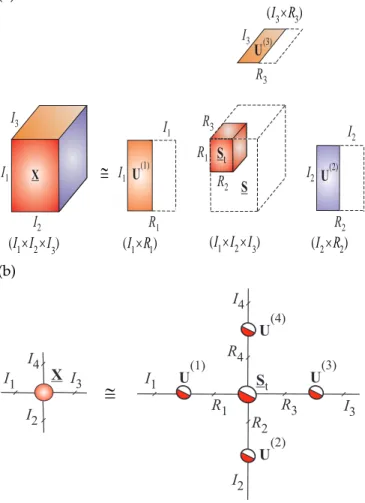
(a) U(1) 1 1 (I R´ ) (I R₂´ ₂) 3 3 (I R´ ) X

@

@

Figure 18:Graphical illustration of the HOSVD. (a) The exact HOSVD and truncated (approximative) HOSVD a for 3rd-order tensor as: X ∼= S_t×₁U(1)_×

2U(2)×3U(3) using a truncated SVD. (b) Tensor network notation for the HOSVD for a 4th-order tensorX∼=S_t×₁U(1)_×

2U(2)×3U(3)×4U(4). All factor matrices U(n) and the core tensor St are orthogonal; due to

orthogonality of the core tensor the HOSVD is unique for a specific multilinear rank.

(1) All orthogonality: Slices in each mode are mutually orthogonal, e.g., for a 3rd-order tensor

hS:,k,:S:,l,:i=0, for k6=l, (17) (2) Pseudo-diagonality: Frobenius norms of slices in each mode are decreasing with the increase of the run-ning index

||S:,k,:||F ≥ ||S:,l,:||F, k≥l. (18)

These norms play a role similar to that of the singular values in the matrix SVD.

The orthogonal matrices U(n) can be in practice computed by the standard SVD or truncated SVD of unfolded mode-n matrices X(n) = U(n)ΣnV(n)T ∈

RIn×I1···In−1In+1···IN_{. After obtaining the orthogonal} ma-tricesU(n)of left singular vectors ofX(n), for eachn, we can compute the core tensor G=Sas

S=X×1U(1)T×2U(2)T· · · ×NU(N)T, (19)

such that

X=S×₁U(1)×₂U(2)· · · ×_NU(N). (20) Due to orthogonality of the core tensorSits slices are mutually orthogonal, this reduces to the diagonality in the matrix case.

In some applications we may use a modified HOSVD in which the SVD can be performed not on the un-folding mode-n matrices X(n) but on their transposes, i.e., X₍T_n) ∼= V(n)ΣnU(n)T. This leads to the modified

HOSVD corresponding to Grassmann manifolds [45], that requires the computation of very large (tall-and-skinny) factor orthogonal matricesV(n)∈RI¯n×In_{, where}

In¯ =∏k6=nIk =I1· · ·In−1In+1· · ·IN, and the core tensor

˜

S∈RI_¯1×I_¯2×···×IN¯ _{based on the following model:}

X=S˜×1V(1)T×2V(2)T· · · ×NV(N)T. (21)

In practical applications the dimensions of unfold-ing matrices X(n) ∈ RIn×In¯ may be prohibitively large (with In¯ In), easily exceeding memory of standard

computers. A truncated SVD of a large-scale unfolding matrix X(n) = U(n)ΣnV(n)T is performed by

partition-ing it into Q slices, as X(n) = [X1,n,X2,n, . . . ,XQ,n] = U(n)Σn[V1,Tn,VT2,n, . . . ,VTQ,n]. Next, the orthogonal

matri-cesU(n)and the diagonal matricesΣnare obtained from

eigenvalue decompositions X(n)XT(n) = U(n)Σ2nU(n)T =

∑qXq,nXTq,n ∈ RIn×In, allowing for the terms Vq,n = X_qT_,nU(n)Σ−1

n to be computed separately. This allows us to

optimize the size of theq-th sliceXq,n∈RIn×(I¯n/Q)so as

to match the available computer memory. Such a simple approach to compute matricesU(n)and/orV(n)does not require loading the entire unfolding matrices at once into computer memory, instead the access to the dataset is sequential. Depending on the size of computer memory, the dimension In is typically less than 10,000, while

there is no limit on the dimension In¯ = ∏k6=nIk. More

sophisticated approaches which also exploit partition of matrices or tensors into blocks for QR/SVD, PCA, NMF/NTF and ICA can be found in [10], [29], [46]–[48]. When a data tensor X is very large and cannot be stored in computer memory, then another challenge is to compute a core tensor G = S by directly using the formula:

G=X×1U(1)T×2U(2)T· · · ×nU(n)T, (22)

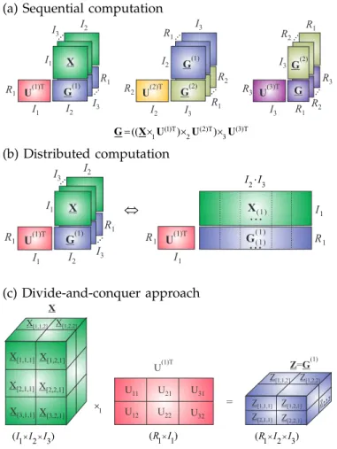
which is generally performed sequentially as illustrated in Fig. 19 (a) and (b) [8], [9].

For very large tensors it is useful to divide the data tensor X into small blocks X[k1,k2,...,kN] and in order to store them on hard disks or distributed memory. In similar way, we can divide the orthogonal factor matrices

U(n)T into corresponding blocks of matrices U(_[kn)T

n,pn] as illustrated in Fig. 19 (c) for 3rd-order tensors [9]. In a general case, we can compute blocks within the resulting

(a) Sequential computation I1 I2 I3 I1 I2 R1 R1 R2 I2 I3 I2 I3 R1 R2 I3 R1 R3 I3 R1 R2 R3 X ... ... ... G(1) G(2) U(1)T G(1) U(2)T G(2) _U(3)T G (1)T (2)T (3)T 1 2 3 (( ) ) = ´ ´ ´ G X U U U I3 ... ... ... R1 R2 (b) Distributed computation

...

...

Figure 19: Computation of a core tensor for a large-scale HOSVD: (a) using sequential computing of multilinear prod-ucts G = S = (((X×₁U(1)T_)×

2U(2)T)×3U(3)T), and (b) by applying fast and distributed implementation of matrix by matrix multiplications; (c) alternative method for very large-scale problems by applying divide and conquer approach, in which a data tensor X and factor matrices U(n)T are par-titioned into suitable small blocks: Subtensors X_[k1,k2,k3] and blocks matrices U(_[k1)T

1,p1], respectively. We compute the blocks

of tensor Z = G(1) = X×₁U(1)T as follows Z_[q1,k2,k3] =

∑K1

k1=1X[k1,k2,k3]×1U (1)T

[k1,q1] (see Eq. (23) for a general case.)

tensor G(n) sequentially or in parallel way as follows:

G(_[kn) 1,k2,...,qn,...,kN] = Kn

∑

If a data tensor has low-multilinear rank, so that its multilinear rank{R1,R2, . . . ,RN}withRnIn, ∀n, we

can further alleviate the problem of dimensionality by first identifying a subtensorW∈RP1×P2×···PN _{for which}

Pn≥Rn, using efficient CUR tensor decompositions [49].

Then the HOSVD can be computed from subtensors as illustrated in Fig. 20 for a 3rd-order tensor. This feature can be formulated in more general form as the following Proposition.

Proposition 1: If a tensor X ∈ RI1×I2×···×IN

has low multilinear rank {R1,R2, . . . ,RN}, with

Figure 20:Alternative approach to computation of the HOSVD for very large data tensor, by exploiting multilinear low-rank approximation. The objective is to select such fibers (up to permutation of fibers) that the subtensorW∈RP1×P2×P3 _with

Pn≥Rn(n=1, 2, 3) has the same multilinear rank{R1,R2,R3} as the whole huge data tensor X, with Rn In. Instead of

unfolding of the whole data tensor X we need to perform unfolding (and applying the standard SVD) for typically much smaller subtensors X(1) = C ∈ RI1×P2×P3_{, X}(2) _{= R ∈} RP1×I2×P3_{, X}(3) _{= T ∈} RP1×P2×I3_{, each in a single}

mode-n, (n = 1, 2, 3). This approach can be applied if data tensor admits low multilinear rank approximation. For simplicity of illustration, we assumed that fibers are permuted in a such way that the firstP−1,P2,P3 fibers were selected.

Rn ≤ In, ∀n, then it can be fully reconstructed

via the HOSVD using only N subtensors

X(n) ∈ RP1×···×Pn−1×In×Pn+1×···×PN_{, (n = 1, 2, . . . ,N),} under the condition that subtensor W ∈ RP1×P2×···×PN_, with Pn ≥ Rn, ∀n has the multilinear rank

{R1,R2, . . . ,RN}.

In practice, we can compute the HOSVD for low-rank, large-scale data tensors in several steps. In the first step, we can apply the CUR FSTD decomposition [49] to identify close to optimal a subtensorW∈RR1×R2×···×RN (see the next Section), In the next step, we can use the standard SVD for unfolding matrices X(₍n_n)₎ of sub-tensors X(n) to compute the left orthogonal matrices

e

U(n) ∈ RIn×Rn_{. Hence, we compute an auxiliary core} tensorG=W×1B(1)· · · ×NB(N), whereB(n)∈RRn×Rn

are inverses of the sub-matrices consisting the first Rn

rows of the matrices Ue(n). In the last step, we perform

HOSVD decomposition of the relatively small core ten-sor as G = S×1Q(1)· · · ×NQ(N), with Q(n) ∈ RRn×Rn

and then desired orthogonal matrices are computed as

U(n)=Ue(n)Q(n).

VII. CUR Tucker Decomposition for Dimensionality

Reduction and Compression of Tensor Data

Note that instead of using the full tensor, we may compute an approximative tensor decomposition model from a limited number of entries (e.g., selected fibers, slices or subtensors). Such completion-type strategies have been developed for low-rank and low-multilinear-rank [50], [51]. A simple approach would be to apply

X

C

U

R

@

J

I

(I C´ )(C R´ ) (R J´ ) Figure 21:CUR decomposition for a huge matrix.

CUR decomposition or Cross-Approximation by sam-pled fibers for the columns of factor matrices in a Tucker approximation [49], [52]. Another approach is to apply tensor networks to represent big data by high-order ten-sors not explicitly but in compressed tensor formats (see next sections). Dimensionality reduction methods are based on the fundamental assumption that large datasets are highly redundant and can be approximated by low-rank matrices and cores, allowing for a significant re-duction in computational complexity and to discover meaningful components while exhibiting marginal loss of information.

For very large-scale matrices, the so called CUR matrix decompositions can be employed for dimensionality re-duction [49], [52]–[55]. Assuming a sufficiently precise low-rank approximation, which implies that data has some internal structure or smoothness, the idea is to provide data representation through a linear combina-tion of a few “meaningful” components, which are exact replicas of columns and rows of the original data matrix [56].

The CUR model, also called skeleton Cross-Approximation, decomposes a data matrix X∈RI×J _as

[53], [54] (see Fig. 21):

X=CUR+E, (24)

whereC∈RI×C_{is a matrix constructed fromCsuitably}

selected columns of the data matrixX,R∈RR×J_consists

of R rows of X, and the matrix U ∈RC×R _{is chosen to}

minimize the norm of the errorE∈RI×J_{. Since typically,} C J and R I, these columns and rows are chosen so as to exhibit high “statistical leverage” and provide the best low-rank fit to the data matrix, at the same time the error cost function ||E||2

F is minimized. For a given

set of columns (C) and rows (R), the optimal choice for the core matrix is U = C†X(R†)T. This requires access to all the entries of Xand is not practical or feasible for large-scale data. A pragmatic choice for the core matrix would be U = W†, where the matrix W ∈ RR×C _is

defined from the intersections of the selected rows and columns. It should be noted that, if rank(X)≤C,R, then the CUR approximation is exact. For the general case, it has been proven that, when the intersection sub-matrix

Wis of maximum volume (the volume of a sub-matrix

W is defined as |det(W)|), this approximation is close to the optimal SVD solution [54].

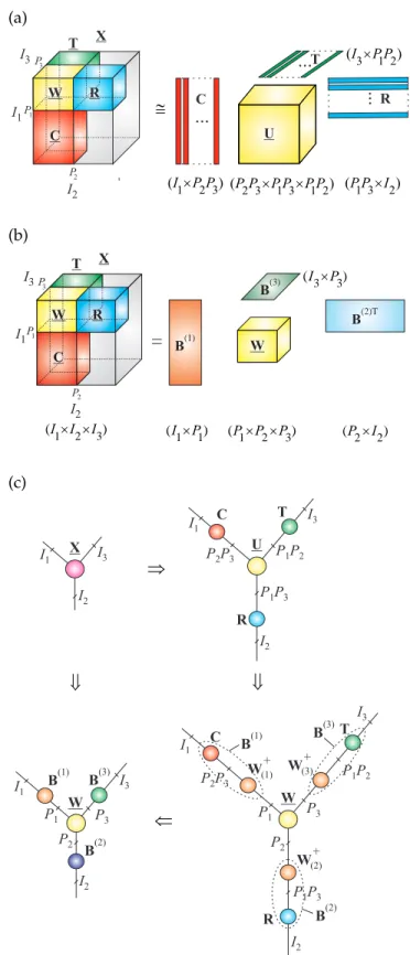
(a) X I3 I1 I2 C R U 1 2 3 (I ´P P) (P P P P P P_{2 3}´ _{1 3}´ _{1 2}) (P P I_{1 3}´ ₂)

...

...

@

...

=

Þ

Ü

ß

ß

Figure 22:(a) CUR decomposition of a large 3rd-order tensor (for simplicity of illustration up to permutation of fibers) X ∼= U×1C×2R×3T = JU;C,R,TK, where U = W×1 W†₍₁₎×₂W†₍₂₎×₃W†₍₃₎ = _JW;W†₍₁₎,W†₍₂₎,W†₍₃₎K. (b) equivalent decomposition expressed via subtensor W, (c) Tensor net-work diagram illustrating transformation from CUR Tucker format (a) to form (b) as: X ∼= W×₁B(1)×₂B(2)×₃B(3) =

JW;CW †