Climate Scenario Development
Co-ordinating Lead Authors
L.O. Mearns, M. Hulme
Lead Authors
T.R. Carter, R. Leemans, M. Lal, P. Whetton
Contributing Authors
L. Hay, R.N. Jones, R. Katz, T. Kittel, J. Smith, R. Wilby
Review Editors
L.J. Mata, J. Zillman
13
Executive Summary 741
13.1 Introduction 743
13.1.1 Definition and Nature of Scenarios 743 13.1.2 Climate Scenario Needs of the Impacts
Community 744
13.2 Types of Scenarios of Future Climate 745 13.2.1 Incremental Scenarios for Sensitivity
Studies 746
13.2.2 Analogue Scenarios 748
13.2.2.1 Spatial analogues 748
13.2.2.2 Temporal analogues 748
13.2.3 Scenarios Based on Outputs from Climate
Models 748
13.2.3.1 Scenarios from General
Circulation Models 748
13.2.3.2 Scenarios from simple climate
models 749
13.2.4 Other Types of Scenarios 749
13.3 Defining the Baseline 749
13.3.1 The Choice of Baseline Period 749
13.3.2 The Adequacy of Baseline Climatological
Data 750
13.3.3 Combining Baseline and Modelled Data 750
13.4 Scenarios with Enhanced Spatial and Temporal
Resolution 751
13.4.1 Spatial Scale of Scenarios 751
13.4.1.1 Regional modelling 751
13.4.1.2 Statistical downscaling 752
13.4.1.3 Applications of the methods to
impacts 752
13.4.2 Temporal Variability 752
13.4.2.1 Incorporation of changes in variability: daily to interannual
time-scales 752
13.4.2.2 Other techniques for incorporating extremes into climate scenarios 754
13.5 Representing Uncertainty in Climate Scenarios 755 13.5.1 Key Uncertainties in Climate Scenarios 755
13.5.1.1 Specifying alternative emissions
futures 755
13.5.1.2 Uncertainties in converting
emissions to concentrations 755
13.5.1.3 Uncertainties in converting
concentrations to radiative forcing 755 13.5.1.4 Uncertainties in modelling the
climate response to a given forcing 755 13.5.1.5 Uncertainties in converting model
response into inputs for impact
studies 756
13.5.2 Approaches for Representing Uncertainties 756 13.5.2.1 Scaling climate model response
patterns 756
13.5.2.2 Defining climate change signals 757 13.5.2.3 Risk assessment approaches 759 13.5.2.4 Annotation of climate scenarios 760
13.6 Consistency of Scenario Components 760
Executive Summary
The Purpose of Climate Scenarios
A climate scenario is a plausible representation of future climate that has been constructed for explicit use in investigating the potential impacts of anthropogenic climate change. Climate scenarios often make use of climate projections (descriptions of the modelled response of the climate system to scenarios of greenhouse gas and aerosol concentrations), by manipulating model outputs and combining them with observed climate data. This new chapter for the IPCC assesses the methods used to develop climate scenarios. Impact assessments have a very wide range of scenario requirements, ranging from global mean estimates of temperature and sea level, through continental-scale descriptions of changes in mean monthly climate, to point or catchment-level detail about future changes in daily or even sub-daily climate.
The science of climate scenario development acts as an important bridge from the climate science of Working Group I to the science of impact, adaptation and vulnerability assess-ment, considered by Working Group II. It also has a close dependence on emissions scenarios, which are discussed by Working Group III.
Methods for Constructing Scenarios
Useful information about possible future climates and their impacts has been obtained using various scenario construction methods. These include climate model based approaches, temporal and spatial analogues, incremental scenarios for sensitivity studies, and expert judgement. This chapter identifies advantages and disadvantages of these different methods (see Table 13.1).
All these methods can continue to serve a useful role in the provision of scenarios for impact assessment, but it is likely that the major advances in climate scenario construction will be made through the refinement and extension of climate model based approaches.
Each new advance in climate model simulations of future climate has stimulated new techniques for climate scenario construction. There are now numerous techniques available for scenario construction, the majority of which ultimately depend upon results obtained from general circulation model (GCM) experiments.
Representing the Cascade of Uncertainty
Uncertainties will remain inherent in predicting future climate change, even though some uncertainties are likely to be narrowed with time. Consequently, a range of climate scenarios should usually be considered in conducting impact assessments.
There is a cascade of uncertainties in future climate predic-tions which includes unknown future emissions of greenhouse gases and aerosols, the conversion of emissions to atmospheric concentrations and to radiative forcing of the climate, modelling the response of the climate system to forcing, and methods for regionalising GCM results.
Scenario construction techniques can be usefully contrasted according to the sources of uncertainty that they address and
those that they ignore. These techniques, however, do not always provide consistent results. For example, simple methods based on direct GCM changes often represent model-to-model differences in simulated climate change, but do not address the uncertainty associated with how these changes are expressed at fine spatial scales. With regionalisation approaches, the reverse is often true. A number of methods have emerged to assist with the quantification and communication of uncertainty in climate scenarios. These include pattern-scaling techniques to inter-polate/extrapolate between results of model experiments, climate scenario generators, risk assessment frameworks and the use of expert judgement. The development of new or refined scenario construction techniques that can account for multiple uncertain-ties merits further investigation.
Representing High Spatial and Temporal Resolution Information
The incorporation of climate changes at high spatial (e.g., tens of kilometres) and temporal (e.g., daily) resolution in climate scenarios currently remains largely within the research domain of climate scenario development. Scenarios containing such high resolution information have not yet been widely used in compre-hensive policy relevant impact assessments.
Preliminary evidence suggests that coarse spatial resolution AOGCM (Atmosphere-Ocean General Circulation Model) information for impact studies needs to be used cautiously in regions characterised by pronounced sub-GCM grid scale variability in forcings. The use of suitable regionalisation techniques may be important to enhance the AOGCM results over such regions.
Incorporating higher resolution information in climate scenarios can substantially alter the assessment of impacts. The incorporation of such information in scenarios is likely to become increasingly common and further evaluation of the relevant methods and their added value in impact assessment is warranted.
Representing Extreme Events
Extreme climate/weather events are very important for most climate change impacts. Changes in the occurrence and intensity of extremes should be included in climate scenarios whenever possible.
Some extreme events are easily or implicitly incorporated in climate scenarios using conventional techniques. It is more difficult to produce scenarios of complex events, such as tropical cyclones and ice storms, which may require specialised techniques. This constitutes an important methodological gap in scenario development. The large uncertainty regarding future changes in some extreme events exacerbates the difficulty in incorporating such changes in climate scenarios.
Applying Climate Scenarios in Impact Assessments
There is no single “best” scenario construction method appropriate for all applications. In each case, the appropriate method is determined by the context and the application of the scenario.
The choice of method constrains the sources of uncertainty that can be addressed. Relatively simple techniques, such as those that rely on scaled or unscaled GCM changes, may well be the
most appropriate for applications in integrated assessment modelling or for informing policy; more sophisticated techniques, such as regional climate modelling or conditioned stochastic weather generation, are often necessary for applications involving detailed regional modelling of climate change impacts.
Improving Information Required for Scenario Development
Improvements in global climate modelling will bring a variety of benefits to most climate scenario development
methods. A more diverse set of model experiments, such as AOGCMs run under a broader range of forcings and at higher resolutions, and regional climate models run either in ensemble mode or for longer time periods, will allow a wider range of uncertainty to be represented in climate scenarios. In addition, incorporation of some of the physical, biological and socio-economic feedbacks not currently simulated in global models will improve the consistency of different scenario elements.
13.1 Introduction
13.1.1 Definition and Nature of Scenarios
For the purposes of this report, a climate scenario refers to a plausible future climate that has been constructed for explicit use in investigating the potential consequences of anthropogenic climate change. Such climate scenarios should represent future conditions that account for both human-induced climate change and natural climate variability. We distinguish a climate scenario from a climate projection (discussed in Chapters 9 and 10), which refers to a description of the response of the climate system to a scenario of greenhouse gas and aerosol emissions, as simulated by a climate model. Climate projections alone rarely provide sufficient information to estimate future impacts of climate change; model outputs commonly have to be manipulated and combined with observed climate data to be usable, for example, as inputs to impact models.
To further illustrate this point, Box 13.1 presents a simple example of climate scenario construction based on climate projections. The example also illustrates some other common considerations in performing an impact assessment that touch on issues discussed later in this chapter.
We also distinguish between a climate scenario and a climate change scenario. The latter term is sometimes used in the scientific literature to denote a plausible future climate. However, this term should strictly refer to a representation of the difference between some plausible future climate and the current or control climate (usually as represented in a climate model) (see Box 13.1, Figure 13.1a). A climate change scenario can be viewed as an interim step toward constructing a climate scenario. Usually a climate scenario requires combining the climate change scenario with a description of the current climate as represented by climate observations (Figure 13.1b). In a climate impacts context, it is the contrasting effects of these two climates – one current (the observed “baseline” climate), one
Box 13.1: Example of scenario construction.
Example of basic scenario construction for an impact study: the case of climate change and world food supply (Rosenzweig and Parry, 1994).
Aim of the study
The objective of this study was to estimate how global food supply might be affected by greenhouse gas induced climate change up to the year 2060. The method adopted involved estimating the change in yield of major crop staples under various scenarios using crop models at 112 representative sites distributed across the major agricultural regions of the world. Yield change estimates were assumed to be applicable to large regions to produce estimates of changes in total production which were then input to a global trade model. Using assumptions about future population, economic growth, trading conditions and technological progress, the trade model estimated plausible prices of food commodities on the international market given supply as defined by the production estimates. This information was then used to define the number of people at risk from hunger in developing countries.
Scenario information
Each of the stages of analysis required scenario information to be provided, including:
• scenarios of carbon dioxide (CO2) concentration, affecting crop growth and water use, as an input to the crop models;
• climate observations and scenarios of future climate, for the crop model simulations;
• adaptation scenarios (e.g., new crop varieties, adjusted farm management) as inputs to the crop models; • scenarios of regional population and global trading policy as an input to the trade model.
To the extent possible, the scenarios were mutually consistent, such that scenarios of population (United Nations medium range estimate) and Gross Domestic Product (GDP) (moderate growth) were broadly in line with the transient scenario of greenhouse gas emissions (based on the Goddard Institute for Space Studies (GISS) scenario A, see Hansen et al., 1988), and hence CO2
concen-trations. Similarly, the climate scenarios were based on 2×CO2 equilibrium GCM projections from three models, where the
radiative forcing of climate was interpreted as the combined concentrations of CO2 (555 ppm) and other greenhouse gases
(contributing about 15% of the change in forcing) equivalent to a doubling of CO2, assumed to occur in about 2060.
Construction of the climate scenario
Since projections of current (and hence future) regional climate from the GCM simulations were not accurate enough to be used directly as an input to the crop model, modelled changes in climate were applied as adjustments to the observed climate at a location. Climate change by 2060 was computed as the difference (air temperature) or ratio (precipitation and solar radiation) of monthly mean climate between the GCM (unforced) control and 2×CO2simulations at GCM grid boxes coinciding with the crop
modelling sites (Figure 13.1b). These estimates were used to adjust observed time-series of daily climate for the baseline period (usually 1961 to 1990) at each site (Figure 13.1b,c). Crop model simulations were conducted for the baseline climate and for each of the three climate scenarios, with and without CO2enrichment (to estimate the relative contributions of CO2and climate to crop
future (the climate scenario) – on the exposure unit1 that
determines the impact of the climate change (Figure 13.1c). A treatment of climate scenario development, in this specific sense, has been largely absent in the earlier IPCC Assessment Reports. The subject has been presented in independent IPCC Technical Guidelines documents (IPCC, 1992, 1994), which were briefly summarised in the Second Assessment Report of Working Group II (Carter et al., 1996b). These documents, while serving a useful purpose in providing guidelines for scenario use,
did not fully address the science of climate scenario development. This may be, in part, because the field has been slow to develop and because only recently has a critical mass of important research issues coalesced and matured such that a full chapter is now warranted.
The chapter also serves as a bridge between this Report of Working Group I and the IPCC Third Assessment Report of Working Group II (IPCC, 2001) (hereafter TAR WG II) of climate change impacts, adaptation and vulnerability. As such it also embodies the maturation in the IPCC assessment process – that is, a recognition of the interconnections among the different segments of the assessment process and a desire to further integrate these segments. Chapter 3 performs a similar role in the TAR WG II (Carter and La Rovere, 2001) also discussing climate scenarios, but treating, in addition, all other scenarios (socio-economic, land use, environmental, etc.) needed for undertaking policy-relevant impact assessment. Chapter 3 serves in part as the other half of the bridge between the two Working Group Reports. Scenarios are neither predictions nor forecasts of future conditions. Rather they describe alternative plausible futures that conform to sets of circumstances or constraints within which they occur (Hammond, 1996). The true purpose of scenarios is to illuminate uncertainty, as they help in determining the possible ramifications of an issue (in this case, climate change) along one or more plausible (but indeterminate) paths (Fisher, 1996).
Not all possibly imaginable futures can be considered viable scenarios of future climate. For example, most climate scenarios include the characteristic of increased lower tropospheric temper-ature (except in some isolated regions and physical circum-stances), since most climatologists have very high confidence in that characteristic (Schneider et al., 1990; Mahlman, 1997). Given our present state of knowledge, a scenario that portrayed global tropospheric cooling for the 21st century would not be viable. We shall see in this chapter that what constitutes a viable scenario of future climate has evolved along with our understanding of the climate system and how this understanding might develop in the future.
It is worth noting that the development of climate scenarios predates the issue of global warming. In the mid-1970s, for example, when a concern emerged regarding global cooling due to the possible effect of aircraft on the stratosphere, simple incremental scenarios of climate change were formulated to evaluate what the possible effects might be worldwide (CIAP, 1975).
The purpose of this chapter is to assess the current state of climate scenario development. It discusses research issues that are addressed by researchers who develop climate scenarios and that must be considered by impacts researchers when they select scenarios for use in impact assessments. This chapter is not concerned, however, with presenting a comprehensive set of climate scenarios for the IPCC Third Assessment Report.
13.1.2 Climate Scenario Needs of the Impacts Community
The specific climate scenario needs of the impacts community vary, depending on the geographic region considered, the type of impact, and the purpose of the study. For example, distinctions
(a)
(b)
(c)
Figure 13.1:Example of the stages in the formation of a simple climate scenario for temperature using Poza Rica (20.3° N, 97.3° W) as a typical site used in the Mexican part of the Rosenzweig and Parry (1994) study.
(a) Mean monthly differences (∆) (2×CO2minus control) of average
temperature (°C) as calculated from the control and 2×CO2runs of the
Geophysical Fluid Dynamics Laboratory (GFDL) GCM (Manabe and Wetherald, 1987) for the model grid box that includes the geographic location of Poza Rica. The climate model spatial resolution is 4.4° latitude by 7.5° longitude.
(b) The average 17-year (1973 to 1989) observed mean monthly maximum temperature for Poza Rica (solid line) and the 2×CO2mean monthly maximum temperature produced by adding the differences portrayed in (a) to this baseline (dashed line). The crop models, however, require daily climate data for input.
(c) A sample of one year’s (1975) observed daily maximum tempera-ture data (solid line) and the 2×CO2daily values created by adding the monthly differences in a) to the daily data (dashed line). Thus, the dashed line is the actual daily maximum temperature time-series describing future climate that was used as one of the weather inputs to the crop models for this study and for this location (see Liverman et al., 1994 for further details).
1An exposure unit is an activity, group, region or resource exposed to
can be made between scenario needs for research in climate scenario development and in the methods of conducting impact assessment (e.g., Woo, 1992; Mearns et al., 1997) and scenario needs for direct application in policy relevant impact and integrated assessments (e.g., Carter et al., 1996a; Smith et al., 1996; Hulme and Jenkins, 1998).
The types of climate variables needed for quantitative impacts studies vary widely (e.g., White, 1985). However, six “cardinal” variables can be identified as the most commonly requested: maximum and minimum temperature, precipitation, incident solar radiation, relative humidity, and wind speed. Nevertheless, this list is far from exhaustive. Other climate or climate-related variables of importance may include CO2
concentration, sea-ice extent, mean sea level pressure, sea level, and storm surge frequencies. A central issue regarding any climate variable of importance for impact assessment is determining at what spatial and temporal scales the variable in question can sensibly be provided, in comparison to the scales most desired by the impacts community. From an impacts perspective, it is usually desirable to have a fair amount of regional detail of future climate and to have a sense of how climate variability (from short to long time-scales) may change. But the need for this sort of detail is very much a function of the scale and purpose of the particular impact assessment. Moreover, the availability of the output from climate models and the advisability of using climate model results at particular scales, from the point of view of the climate modellers, ultimately determines what scales can and should be used.
Scenarios should also provide adequate quantitative measures of uncertainty. The sources of uncertainty are many, including the
trajectory of greenhouse gas emissions in the future, their conver-sion into atmospheric concentrations, the range of responses of various climate models to a given radiative forcing and the method of constructing high resolution information from global climate model outputs (Pittock, 1995; see Figure 13.2). For many purposes, simply defining a single climate future is insufficient and unsatisfactory. Multiple climate scenarios that address at least one, or preferably several sources of uncertainty allow these uncertainties to be quantified and explicitly accounted for in impact assessments. Moreover, a further important requirement for impact assessments is to ensure consistency is achieved among various scenario components, such as between climate change, sea level rise and the concentration of actual (as opposed to equivalent) CO2implied by a particular emissions scenario.
As mentioned above, climate scenarios that are developed for impacts applications usually require that some estimate of climate change be combined with baseline observational climate data, and the demand for more complete and sophisticated observational data sets of climate has grown in recent years. The important considerations for the baseline include the time period adopted as well as the spatial and temporal resolution of the baseline data.
Much of this chapter is devoted to assessing how and how successfully these needs and requirements are currently met.
13.2 Types of Scenarios of Future Climate
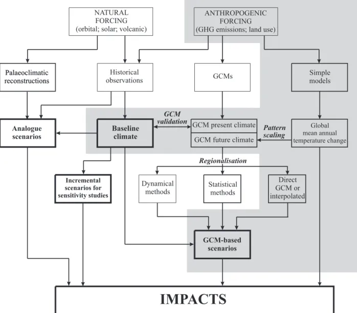
Four types of climate scenario that have been applied in impact assessments are introduced in this section. The most common scenario type is based on outputs from climate models and receives most attention in this chapter. The other three types have usually been applied with reference to or in conjunction with model-based scenarios, namely: incremental scenarios for sensitivity studies, analogue scenarios, and a general category of “other scenarios”. The origins of these scenarios and their mutual linkages are depicted in Figure 13.3.
The suitability of each type of scenario for use in policy-relevant impact assessment can be assessed according to five criteria adapted from Smith and Hulme (1998):
1. Consistencyat regional level with global projections. Scenario changes in regional climate may lie outside the range of global mean changes but should be consistent with theory and model-based results.
2. Physical plausibility and realism. Changes in climate should be physically plausible, such that changes in different climatic variables are mutually consistent and credible.
3. Appropriateness of information for impact assessments.
Scenarios should present climate changes at an appropriate temporal and spatial scale, for a sufficient number of variables, and over an adequate time horizon to allow for impact assess-ments.
4. Representativeness of the potential range of future regional
climate change.
5. Accessibility. The information required for developing climate scenarios should be readily available and easily accessible for use in impact assessments.
Socio-economic assumptions
(WGII/Ch 3; WGIII/Ch 2 - SRES)
Emissions scenarios
(WGIII/Ch 2 - SRES)
Concentration projections
(WGI/Ch 3,4,5)
Radiative forcing projections
(WGI/Ch 6)
Climate projections
(WGI/Ch 8,9,10)
Sea level projections
(WGI/Ch 11)
Global change scenarios
(WGII/Ch 3) Interactions and feedbacks (WGI/Ch 3,4,5,7; WGII/Ch3) Impacts (WGII) Climate scenarios (WGI/Ch 13) Policy responses: adaptation and mitigation (WGII; WGIII)
Figure 13.2: The cascade of uncertainties in projections to be consid-ered in developing climate and related scenarios for climate change impact, adaptation and mitigation assessment.
A summary of the major advantages and disadvantages of different scenario development methods, based on these criteria, is presented in Table 13.1. The relative significance of the advantages and disadvantages is highly application dependent.
13.2.1 Incremental Scenarios for Sensitivity Studies
Incremental scenarios describe techniques where particular climatic (or related) elements are changed incrementally by plausible though arbitrary amounts (e.g., +1, +2, +3, +4°C change in temperature). Also referred to as synthetic scenarios (IPCC, 1994), they are commonly applied to study the sensitivity of an exposure unit to a wide range of variations in climate, often according to a qualitative interpretation of projections of future regional climate from climate model simulations (“guided sensitivity analysis”, see IPCC-TGCIA, 1999). Incremental scenarios facilitate the construction of response surfaces – graphical devices for plotting changes in climate against some
measure of impact (for example see Figure 13.9b) which can assist in identifying critical thresholds or discontinuities of response to a changing climate. Other types of scenarios (e.g., based on model outputs) can be superimposed on a response surface and the significance of their impacts readily evaluated (e.g., Fowler, 1999). Most studies have adopted incremental scenarios of constant changes throughout the year (e.g., Terjung
et al., 1984; Rosenzweig et al., 1996), but some have introduced seasonal and spatial variations in the changes (e.g., Whetton et al., 1993; Rosenthal et al., 1995) and others have examined arbitrary changes in interannual, within-month and diurnal variability as well as changes in the mean (e.g., Williams et al., 1988; Mearns et al., 1992; Semenov and Porter, 1995; Mearns et al., 1996).
Incremental scenarios provide information on an ordered range of climate changes and can readily be applied in a consis-tent and replicable way in different studies and regions, allowing for direct intercomparison of results. However, such scenarios do Palaeoclimatic
reconstructions observationsHistorical GCMs modelsSimple
IMPACTS
Analoguescenarios Baselineclimate
GCM present climate Global
mean annual temperature change Incremental scenarios for sensitivity studies Direct GCM or interpolated Statistical methods Dynamical methods GCM-based scenarios GCM future climate Palaeoclimatic reconstructions NATURAL FORCING (orbital; solar; volcanic)
ANTHROPOGENIC FORCING (GHG emissions; land use)
GCM validation
Pattern scaling Regionalisation
Figure 13.3:Some alternative data sources and procedures for constructing climate scenarios for use in impact assessment. Highlighted boxes indicate the baseline climate and common types of scenario (see text for details). Grey shading encloses the typical components of climate scenario generators.
Table 13.1: The role of various types of climate scenarios and an evaluation of their advantages and disadvantages according to the five criteria described in the text. Note that in some applications a combination of methods may be used (e.g., regional modelling and a weather generator).
Scenario type or tool Description/Use Advantagesa Disadvantagesa
Incremental •Testing system sensitivity
•Identifying key climate
thresholds
• Easy to design and apply (5)
• Allows impact response surfaces to be created (3)
•Potential for creating unrealistic scenarios (1, 2)
•Not directly related to greenhouse gas forcing (1)
Analogue:
Palaeoclimatic •Characterising warmer
periods in past
• A physically plausible changed climate that really
did occur in the past of a magnitude similar to that predicted for ~2100 (2)
•Variables may be poorly resolved in space and
time (3, 5)
•Not related to greenhouse gas forcing (1)
Instrumental •Exploring vulnerabilities
and some adaptive capacities
• Physically realistic changes (2)
• Can contain a rich mixture of well-resolved,
internally consistent, variables (3)
• Data readily available (5)
•Not necessarily related to greenhouse gas forcing (1)
•Magnitude of the climate change usually quite
small (1)
•No appropriate analogues may be available (5)
Spatial •Extrapolating
climate/ecosystem relationships
•Pedagogic
• May contain a rich mixture of well-resolved
variables (3)
•Not related to greenhouse gas forcing (1, 4)
•Often physically implausible (2)
•No appropriate analogues may be available (5)
Climate model based:
Direct AOGCM outputs •Starting point for most
climate scenarios
•Large-scale response to
anthropogenic forcing
• Information derived from the most
comprehensive, physically-based models (1, 2)
• Long integrations (1)
• Data readily available (5)
• Many variables (potentially) available (3)
•Spatial information is poorly resolved (3)
•Daily characteristics may be unrealistic except for
very large regions (3)
•Computationally expensive to derive multiple
scenarios (4, 5)
•Large control run biases may be a concern for use
in certain regions (2) High resolution/stretched
grid (AGCM)
•Providing high resolution
information at global/continental scales
• Provides highly resolved information (3)
• Information is derived from physically-based
models (2)
• Many variables available (3)
• Globally consistent and allows for feedbacks (1,2)
•Computationally expensive to derive multiple
scenarios (4, 5)
•Problems in maintaining viable parametrizations
across scales (1,2)
•High resolution is dependent on SSTs and sea ice
margins from driving model (AOGCM) (2)
•Dependent on (usually biased) inputs from driving
AOGCM(2)
Regional models •Providing high
spatial/temporal resolution information
• Provides very highly resolved information (spatial
and temporal) (3)
• Information is derived from physically-based
models (2)
• Many variables available (3)
• Better representation of some weather extremes
than in GCMs (2, 4)
•Computationally expensive, and thus few multiple scenarios (4, 5)
•Lack of two-way nesting may raise concern
regarding completeness (2)
•Dependent on (usually biased) inputs from driving
AOGCM(2) Statistical downscaling •Providing point/high
spatial resolution information
• Can generate information on high resolution grids, or non-uniform regions (3)
• Potential,for some techniques, to address a diverse range of variables (3)
• Variables are (probably) internally consistent (2)
• Computationally (relatively) inexpensive (5)
• Suitable for locations with limited computational resources (5)
• Rapid application to multiple GCMs (4)
•Assumes constancy of empirical relationships in the future (1, 2)
•Demands access to daily observational surface and/or upper air data that spans range of variability (5)
•Not many variables produced for some techniques (3, 5)
•Dependent on (usually biased) inputs from driving AOGCM(2) Climate scenario generators •Integrated assessments •Exploring uncertainties •Pedagogic
• May allow for sequential quantification of uncertainty (4)
• Provides ‘integrated’ scenarios (1)
• Multiple scenarios easy to derive (4)
•Usually rely on linear pattern scaling methods (1)
•Poor representation of temporal variability (3)
•Low spatial resolution (3)
Weather generators •Generating baseline
climate time-series
•Altering higher order moments of climate
•Statistical downscaling
• Generates long sequences of daily or sub-daily climate (2, 3)
• Variables are usually internally consistent (2)
• Can incorporate altered frequency/intensity of ENSO events (3)
•Poor representation of low frequency climate variability (2, 4)
•Limited representation of extremes (2, 3, 4)
•Requires access to long observational weather series (5)
•In the absence of conditioning, assumes constant statistical characteristics (1, 2)
Expert judgment •Exploring probability and
risk
•Integrating current thinking on changes in climate
• May allow for a ‘consensus’ (4)
• Has the potential to integrate a very broad range of relevant information (1, 3, 4)
• Uncertainties can be readily represented (4)
•Subjectivity may introduce bias (2)
•A representative survey of experts may be difficult to implement (5)
a Numbers in parentheses under Advantages and Disadavantages indicate that they are relevant to the criteria described. The five criteria are: (1)
Consistency at regional level with global projections; (2) Physical plausibility and realism, such that changes in different climatic variables are mutually consistent and credible, and spatial and temporal patterns of change are realistic; (3) Appropriateness of information for impact assessments (i.e., resolution, time horizon, variables); (4) Representativeness of the potential range of future regional climate change; and (5) Accessibility for use in impact assessments.
not necessarily present a realistic set of changes that are physically plausible. They are usually adopted for exploring system sensitivity prior to the application of more credible, model-based scenarios (Rosenzweig and Iglesias, 1994; Smith and Hulme, 1998).
13.2.2 Analogue Scenarios
Analogue scenarios are constructed by identifying recorded climate regimes which may resemble the future climate in a given region. Both spatial and temporal analogues have been used in constructing climate scenarios.
13.2.2.1 Spatial analogues
Spatial analogues are regions which today have a climate analogous to that anticipated in the study region in the future. For example, to project future grass growth, Bergthórsson et al.
(1988) used northern Britain as a spatial analogue for the potential future climate over Iceland. Similarly, Kalkstein and Greene (1997) used Atlanta as a spatial analogue of New York in a heat/mortality study for the future. Spatial analogues have also been exploited along altitudinal gradients to project vegetation composition, snow conditions for skiing, and avalanche risk (e.g., Beniston and Price, 1992; Holten and Carey, 1992; Gyalistras et al., 1997). However, the approach is severely restricted by the frequent lack of correspondence between other important features (both climatic and non-climatic) of a study region and its spatial analogue (Arnell et al., 1990). Thus, spatial analogues are seldom applied as scenarios,per se. Rather, they are valuable for validating the extrapolation of impact models by providing information on the response of systems to climatic conditions falling outside the range currently experienced at a study location.
13.2.2.2 Temporal analogues
Temporal analogues make use of climatic information from the past as an analogue for possible future climate (Webb and Wigley, 1985; Pittock, 1993). They are of two types: palaeo-climatic analogues and instrumentally based analogues.
Palaeoclimatic analogues are based on reconstructions of past climate from fossil evidence, such as plant or animal remains and sedimentary deposits. Two periods have received particular attention (Budyko, 1989; Shabalova and Können, 1995): the mid-Holocene (about 5 to 6 ky BP2) and the Last (Eemian)
Interglacial (about 120 to 130 ky BP). During these periods, mean global temperatures were as warm as or warmer than today (see Chapter 2, Section 2.4.4), perhaps resembling temperatures anticipated during the 21st century. Palaeoclimatic analogues have been adopted extensively in the former Soviet Union (e.g., Frenzel et al., 1992; Velichko et al., 1995a,b; Anisimov and Nelson, 1996), as well as elsewhere (e.g., Kellogg and Schware, 1981; Pittock and Salinger, 1982). The major disadvantage of using palaeoclimatic analogues for climate scenarios is that the causes of past changes in climate (e.g., variations in the Earth’s orbit about the Sun; continental configuration) are different from
those posited for the enhanced greenhouse effect, and the resulting regional and seasonal patterns of climate change may be quite different (Crowley, 1990; Mitchell, 1990). There are also large uncertainties about the quality of many palaeoclimatic reconstructions (Covey, 1995). However, these scenarios remain useful for providing insights about the vulnerability of systems to abrupt climate change (e.g., Severinghaus et al., 1998) and to past El Niño-Southern Oscillation (ENSO) extremes (e.g., Fagan, 1999; Rodbell et al., 1999). They also can provide valuable information for testing the ability of climate models to reproduce past climate fluctuations (see Chapter 8).
Periods of observed global scale warmth during the historical period have also been used as analogues of a greenhouse gas induced warmer world (Wigley et al., 1980). Such scenarios are usually constructed by estimating the difference between the regional climate during the warm period and that of the long-term average or a similarly selected cold period (e.g., Lough et al., 1983). An alternative approach is to select the past period on the basis not only of the observed climatic conditions but also of the recorded impacts (e.g., Warrick, 1984; Williams et al., 1988; Rosenberg et al., 1993; Lapin et al., 1995). A further method employs observed atmospheric circulation patterns as analogues (e.g., Wilby et al., 1994). The advantage of the analogue approach is that the changes in climate were actually observed and so, by definition, are internally consistent and physically plausible. Moreover, the approach can yield useful insights into past sensitivity and adaptation to climatic variations (Magalhães and Glantz, 1992). The major objection to these analogues is that climate anomalies during the past century have been fairly minor compared to anticipated future changes, and in many cases the anomalies were probably associated with naturally occurring changes in atmospheric circulation rather than changes in greenhouse gas concentrations (e.g., Glantz, 1988; Pittock, 1989).
13.2.3 Scenarios Based on Outputs from Climate Models
Climate models at different spatial scales and levels of complexity provide the major source of information for constructing scenarios. GCMs and a hierarchy of simple models produce information at the global scale. These are discussed further below and assessed in detail in Chapters 8 and 9. At the regional scale there are several methods for obtaining sub-GCM grid scale information. These are detailed in Chapter 10 and summarised in Section 13.4.
13.2.3.1 Scenarios from General Circulation Models
The most common method of developing climate scenarios for quantitative impact assessments is to use results from GCM experiments. GCMs are the most advanced tools currently available for simulating the response of the global climate system to changing atmospheric composition.
All of the earliest GCM-based scenarios developed for impact assessment in the 1980s were based on equilibrium-response experiments (e.g., Emanuel et al., 1985; Rosenzweig, 1985; Gleick, 1986; Parry et al., 1988). However, most of these scenarios contained no explicit information about the time of
realisation of changes, although time-dependency was introduced in some studies using pattern-scaling techniques (e.g., Santer et al., 1990; see Section 13.5).
The evolving (transient) pattern of climate response to gradual changes in atmospheric composition was introduced into climate scenarios using outputs from coupled AOGCMs from the early 1990s onwards. Recent AOGCM simulations (see Chapter 9, Table 9.1) begin by modelling historical forcing by greenhouse gases and aerosols from the late 19th or early 20th century onwards. Climate scenarios based on these simulations are being increasingly adopted in impact studies (e.g., Neilson et al., 1997; Downing et al., 2000) along with scenarios based on ensemble simulations (e.g., papers in Parry and Livermore, 1999) and scenarios accounting for multi-decadal natural climatic variability from long AOGCM control simulations (e.g., Hulme
et al., 1999a).
There are several limitations that restrict the usefulness of AOGCM outputs for impact assessment: (i) the large resources required to undertake GCM simulations and store their outputs, which have restricted the range of experiments that can be conducted (e.g., the range of radiative forcings assumed); (ii) their coarse spatial resolution compared to the scale of many impact assessments (see Section 13.4); (iii) the difficulty of distinguishing an anthropogenic signal from the noise of natural internal model variability (see Section 13.5); and (iv) the differ-ence in climate sensitivity between models.
13.2.3.2 Scenarios from simple climate models
Simple climate models are simplified global models that attempt to reproduce the large-scale behaviour of AOGCMs (see Chapter 9). While they are seldom able to represent the non-linearities of some processes that are captured by more complex models, they have the advantage that multiple simulations can be conducted very rapidly, enabling an exploration of the climatic effects of alternative scenarios of radiative forcing, climate sensitivity and other parametrized uncertainties (IPCC, 1997). Outputs from these models have been used in conjunction with GCM informa-tion to develop scenarios using pattern-scaling techniques (see Section 13.5). They have also been used to construct regional greenhouse gas stabilisation scenarios (e.g., Gyalistras and Fischlin, 1995). Simple climate models are used in climate scenario generators (see Section 13.5.2) and in some integrated assessment models (see Section 13.6).
13.2.4 Other Types of Scenarios
Three additional types of climate scenarios have also been adopted in impact studies. The first type involves extrapolating ongoing trends in climate that have been observed in some regions and that appear to be consistent with model-based projections of climate change (e.g., Jones et al., 1999). There are obvious dangers in relying on extrapolated trends, and especially in assuming that recent trends are due to anthropogenic forcing rather than natural variability (see Chapters 2 and 12). However, if current trends in climate are pointing strongly in one direction, it may be difficult to defend the credibility of scenarios that posit a trend in the opposite direction, especially over a short projection period.
A second type of scenario, which has some resemblance to the first, uses empirical relationships between regional climate and global mean temperature from the instrumental record to extrapolate future regional climate on the basis of projected global or hemispheric mean temperature change (e.g. Vinnikov and Groisman, 1979; Anisimov and Poljakov, 1999). Again, this method relies on the assumption that past relationships between local and broad-scale climate are also applicable to future conditions.
A third type of scenario is based on expert judgement, whereby estimates of future climate change are solicited from climate scientists, and the results are sampled to obtain probability density functions of future change (NDU, 1978; Morgan and Keith, 1995; Titus and Narayanan, 1996; Kuikka and Varis, 1997; Tol and de Vos, 1998). The main criticism of expert judgement is its inherent subjectivity, including problems of the representativeness of the scientists sampled and likely biases in questionnaire design and analysis of the responses (Stewart and Glantz, 1985). Nevertheless, since uncertainties in estimates of future climate are inevitable, any moves towards expressing future climate in probabilistic terms will necessarily embrace some elements of subjective judgement (see Section 13.5).
13.3 Defining the Baseline
A baseline period is needed to define the observed climate with which climate change information is usually combined to create a climate scenario. When using climate model results for scenario construction, the baseline also serves as the reference period from which the modelled future change in climate is calculated.
13.3.1 The Choice of Baseline Period
The choice of baseline period has often been governed by availability of the required climate data. Examples of adopted baseline periods include 1931 to 1960 (Leemans and Solomon, 1993), 1951 to 1980 (Smith and Pitts, 1997), or 1961 to 1990 (Kittel et al., 1995; Hulme et al., 1999b).
There may be climatological reasons to favour earlier baseline periods over later ones (IPCC, 1994). For example, later periods such as 1961 to 1990 are likely to have larger anthropogenic trends embedded in the climate data, especially the effects of sulphate aerosols over regions such as Europe and eastern USA (Karl et al., 1996). In this regard, the “ideal” baseline period would be in the 19th century when anthropogenic effects on global climate were negligible. Most impact assessments, however, seek to determine the effect of climate change with respect to “the present”, and therefore recent baseline periods such as 1961 to 1990 are usually favoured. A further attraction of using 1961 to 1990 is that observational climate data coverage and availability are generally better for this period compared to earlier ones.
Whatever baseline period is adopted, it is important to acknowledge that there are differences between climatological averages based on century-long data (e.g., Legates and Wilmott, 1990) and those based on sub-periods. Moreover, different 30-year periods have been shown to exhibit differences in regional annual mean baseline temperature and precipitation of up to
±0.5ºC and ±15% respectively (Hulme and New, 1997; Visser et al., 2000; see also Chapter 2).
13.3.2 The Adequacy of Baseline Climatological Data
The adequacy of observed baseline climate data sets can only be evaluated in the context of particular climate scenario construction methods, since different methods have differing demands for baseline climate data.
There are an increasing number of gridded global (e.g., Leemans and Cramer, 1991; New et al., 1999) and national (e.g., Kittel et al., 1995, 1997; Frei and Schär, 1998) climate data sets describing mean surface climate, although few describe inter-annual climate variability (see Kittel et al., 1997; Xie and Arkin, 1997; New et al., 2000). Differences between alternative gridded regional or global baseline climate data sets may be large, and these may induce non-trivial differences in climate change impacts that use climate scenarios incorporating different baseline climate data (e.g., Arnell, 1999). These differences may be as much a function of different interpolation methods and station densities as they are of errors in observations or the result of sampling different time periods (Hulme and New, 1997; New, 1999). A common problem that some methods endeavour to correct is systematic biases in station locations (e.g., towards low elevation sites). The adequacy of different techniques (e.g., Daly
et al., 1994; Hutchinson, 1995; New et al., 1999) to interpolate station records under conditions of varying station density and/or different topography has not been systematically evaluated.
A growing number of climate scenarios require gridded daily baseline climatological data sets at continental or global scales yet, to date, the only observed data products that meet this criterion are experimental (e.g., Piper and Stewart, 1996; Widmann and Bretherton, 2000). For this and other reasons, attempts have been made to combine monthly observed climatolo-gies with stochastic weather generators to allow “synthetic” daily observed baseline data to be generated for national (e.g., Carter et al., 1996a; Semenov and Brooks, 1999), continental (e.g., Voet et al., 1996; Kittel et al., 1997), or even global (e.g., Friend, 1998) scales. Weather generators are statistical models of observed sequences of weather variables, whose outputs resemble weather data at individual or multi-site locations (Wilks and Wilby, 1999). Access to long observed daily weather series for many parts of the world (e.g., oceans, polar regions and some developing countries) is a problem for climate scenario developers who wish to calibrate and use weather generators.
A number of statistical downscaling techniques (see Section 13.4 and Chapter 10, Section 10.6, for definition) used in scenario development employ Numerical Weather Prediction (NWP) reanalysis data products as a source of upper air climate data (Kalnay et al., 1996). These reanalysis data sets extend over periods up to 40 years and provide spatial and temporal resolution sometimes lacking in observed climate data sets. Relatively little detailed work has compared such reanalysis data with independent observed data sets (see Santer et al., 1999, and Widmann and Bretherton, 2000, for two exceptions), but it is known that certain reanalysis variables −such as precipitation and some other hydrological variables −are unreliable.
13.3.3 Combining Baseline and Modelled Data
Climate scenarios based on model estimates of future climate can be constructed either by adopting the direct model outputs or by combining model estimates of the changed climate with observa-tional climate data. Impact studies rarely use GCM outputs directly because GCM biases are too great and because the spatial resolution is generally too coarse to satisfy the data requirements for estimating impacts. Mearns et al. (1997) and Mavromatis and Jones (1999) provide two of the few examples of using climate model output directly as input into an impact assessment.
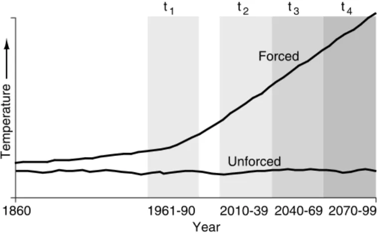
Model-based estimates of climate change should be calculated with respect to the chosen baseline. For example, it would be inappropriate to combine modelled changes in climate calculated with respect to model year 1990 with an observed baseline climate representing 1951 to 1980. Such an approach would “disregard” about 0.15°C of mean global warming occurring between the mid-1970s and 1990. It would be equally misleading to apply modelled changes in climate calculated with respect to an unforced (control) climate representing “pre-industrial” conditions (e.g., “forced” t3 minus “unforced” t1in
Figure 13.4) to an observed baseline climate representing some period in the 20th century. Such an approach would introduce an unwarranted amount of global climate change into the scenario. This latter definition of modelled climate change was originally used in transient climate change experiments to overcome problems associated with climate “drift” in the coupled AOGCM simulations (Cubasch et al., 1992), but was not designed to be used in conjunction with observed climate data. It is more appropriate to define the modelled change in climate with respect to the same baseline period that the observed climate data set is representing (e.g., “forced” t3minus “forced” t1in Figure 13.4,
added to a 1961 to 1990 baseline climate).
Whatever baseline period is selected, there are a number of ways in which changes in climate can be calculated from model results and applied to baseline data. For example, changes in
t1 t2 t3 Forced Unforced 1860 1961-90 2040-69 2070-99 t Year Temperature 2010-39 4
Figure 13.4:A schematic representation of different simulations and periods in a coupled AOGCM climate change experiment that may be used in the definition of modelled climate change. t1to t4define
climate can be calculated either as the difference or as the ratio between the simulated future climate and the simulated baseline climate. These differences or ratios are then applied to the observed baseline climate – whether mean values, monthly or a daily time-series. Differences are commonly applied to tempera-ture (as in Box 13.1), while ratios are usually used with those surface variables, such as precipitation, vapour pressure and radiation, that are either positive or zero. Climate scenarios have been constructed using both absolute and relative changes for precipitation. The effects of the two different approaches on the resulting climate change impacts depend on the types of impacts being studied and the region of application. Some studies report noticeable differences in impacts (e.g., Alcamo et al., 1998), especially since applying ratio changes alters the standard deviation of the original series (Mearns et al., 1996); in others, differences in impacts were negligible (e.g., Torn and Fried, 1992).
13.4 Scenarios with Enhanced Spatial and Temporal Resolution
The spatial and temporal scales of information from GCMs, from which climate scenarios have generally been produced, have not been ideal from an impacts point of view. The desire for informa-tion on climate change regarding changes in variability as well as changes in mean conditions and for information at high spatial resolutions has been consistent over a number of years (Smith and Tirpak, 1989).
The scale at which information can appropriately be taken from relatively coarse-scale GCMs has also been debated. For example, many climate scenarios constructed from GCM outputs have taken information from individual GCM grid boxes, whereas most climate modellers do not consider the outputs from their simulation experiments to be valid on a single grid box scale and usually examine the regional results from GCMs over a cluster of grid boxes (see Chapter 10, Section 10.3). Thus, the scale of information taken from coarse resolution GCMs for scenario development often exceeds the reasonable resolution of accuracy of the models themselves.
In this section we assess methods of incorporating high resolution information into climate scenarios. The issue of spatial and temporal scale embodies an important type of uncertainty in climate scenario development (see Section 13.5.1.5).
Since spatial and temporal scales in atmospheric phenomena are often related, approaches for increasing spatial resolution can also be expected to improve information at high-frequency temporal scales (e.g., Mearns et al., 1997; Semenov and Barrow, 1997; Wang et al., 1999; see also Chapter 10).
13.4.1 Spatial Scale of Scenarios
The climate change impacts community has long bemoaned the inadequate spatial scale of climate scenarios produced from coarse resolution GCM output (Gates, 1985; Lamb, 1987; Robinson and Finkelstein, 1989; Smith and Tirpak, 1989; Cohen, 1990). This dissatisfaction emanates from the perceived mismatch of scale between coarse resolution GCMs (hundreds of
kilometres) and the scale of interest for regional impacts (an order or two orders of magnitude finer scale) (Hostetler, 1994; IPCC, 1994). For example, many mechanistic models used to simulate the ecological effects of climate change operate at spatial resolu-tions varying from a single plant to a few hectares. Their results may be highly sensitive to fine-scale climate variations that may be embedded in coarse-scale climate variations, especially in regions of complex topography, along coastlines, and in regions with highly heterogeneous land-surface covers.
Conventionally, regional “detail” in climate scenarios has been incorporated by applying changes in climate from the coarse-scale GCM grid points to observation points that are distributed at varying resolutions, but often at resolutions higher than that of the GCMs (e.g., see Box 13.1; Whetton et al., 1996; Arnell, 1999). Recently, high resolution gridded baseline climatologies have been developed with which coarse resolution GCM results have been combined (e.g., Saarikko and Carter, 1996; Kittel et al., 1997). Such relatively simple techniques, however, cannot overcome the limitations imposed by the fundamental spatial coarseness of the simulated climate change information itself.
Three major techniques (referred to as regionalisation techniques) have been developed to produce higher resolution climate scenarios: (1) regional climate modelling (Giorgi and Mearns, 1991; McGregor, 1997; Giorgi and Mearns, 1999); (2) statistical downscaling (Wilby and Wigley, 1997; Murphy, 1999); and (3) high resolution and variable resolution Atmospheric General Circulation Model (AGCM) time-slice techniques (Cubasch et al., 1995; Fox-Rabinovitz et al., 1997). The two former methods are dependent on the large-scale circulation variables from GCMs, and their value as a viable means of increasing the spatial resolution of climate change information thus partially depends on the quality of the GCM simulations. The variable resolution and high resolution time-slice methods use the AGCMs directly, run at high or variable resolutions. The high resolution time-slice technique is also dependent on the sea surface temperature simulated by a coarser resolution AOGCM. There have been few completed experiments using these AGCM techniques, which essentially are still under development (see Chapter 10, Section 10.4). Moreover, they have rarely been applied to explicit scenario formation for impacts purposes (see Jendritzky and Tinz, 2000, for an exception) and are not discussed further in this chapter. See Chapter 10 for further details on all techniques.
13.4.1.1 Regional modelling
The basic strategy in regional modelling is to rely on the GCM to reproduce the large-scale circulation of the atmosphere and for the regional model to simulate sub-GCM scale regional distribu-tions or patterns of climate, such as precipitation, temperature, and winds, over the region of interest (Giorgi and Mearns, 1991; McGregor, 1997; Giorgi and Mearns, 1999). The GCM provides the initial and lateral boundary conditions for driving the regional climate model (RCM). In general, the spatial resolution of the regional model is on the order of tens of kiilometres, whereas the GCM scale is an order of magnitude coarser. Further details on the techniques of regional climate modelling are covered in Chapter 10, Section 10.5.
13.4.1.2 Statistical downscaling
In statistical downscaling, a cross-scale statistical relationship is developed between large-scale variables of observed climate such as spatially averaged 500 hPa heights, or measure of vorticity, and local variables such as site-specific temperature and precipitation (von Storch, 1995; Wilby and Wigley, 1997; Murphy, 1999). These relationships are assumed to remain constant in the climate change context. Also, it is assumed that the predictors selected (i.e., the large-scale variables) adequately represent the climate change signal for the predic-tand (e.g., local-scale precipitation). The statistical relationship is used in conjunction with the change in the large-scale variables to determine the future local climate. Further details of these techniques are provided in Chapter 10, Section 10.6.
13.4.1.3 Applications of the methods to impacts
While the two major techniques described above have been available for about ten years, and proponents claim use in impact assessments as one of their important applications, it is only quite recently that scenarios developed using these techniques have actually been applied in a variety of impact assessments, such as temperature extremes (Hennessy et al., 1998; Mearns, 1999); water resources (Hassall and Associates, 1998; Hay et al., 1999; Wang et al., 1999; Wilby et al., 1999; Stone et al., 2001); agriculture (Mearns et al., 1998, 1999, 2000a, 2001; Brown et al., 2000) and forest fires (Wotton et al., 1998). Prior to the past couple of years, these techniques were mainly used in pilot studies focused on increasing the temporal (and spatial) scale of scenarios (e.g., Mearns et al., 1997; Semenov and Barrow, 1997).
One of the most important aspects of this work is determining whether the high resolution scenario actually leads to significantly different calculations of impacts compared to that of the coarser resolution GCM from which the high resolution scenario was partially derived. This aspect is related to the issue of uncertainty in climate scenarios (see Section 13.5). We provide examples of such studies below.
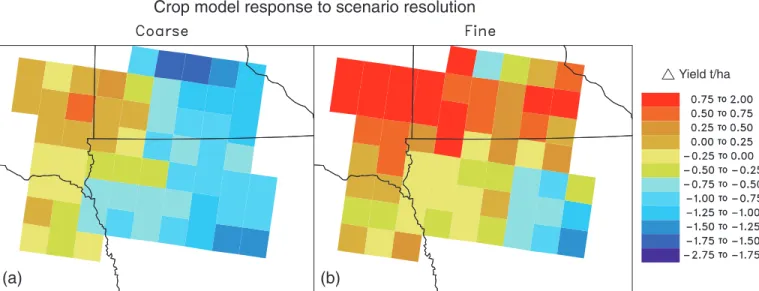
Application of high resolution scenarios produced from a regional model (Giorgi et al., 1998) over the Central Plains of the USA produced changes in simulated crop yields that were significantly different from those changes calculated from a coarser resolution GCM scenario (Mearns et al., 1998; 1999, 2001). For simulated corn in Iowa, for example, the large-scale (GCM) scenario resulted in a statistically significant decrease in yield, but the high resolution scenario produced an insignif-icant increase (Figure 13.5). Substantial differences in regional economic impacts based on GCM and RCM scenarios were also found in a recent integrated assessment of agriculture in the south-eastern USA (Mearns et al., 2000a,b). Hay et al. (1999), using a regression-based statistical downscaling technique, developed downscaled scenarios based on the Hadley Centre Coupled AOGCM (HadCM2) transient runs and applied them to a hydrologic model in three river basins in the USA. They found that the standard scenario from the GCM produced changes in surface runoff that were quite different from those produced from the downscaled scenario (Figure 13.6).
13.4.2 Temporal Variability
The climate change information most commonly taken from climate modelling experiments comprises mean monthly, seasonal, or annual changes in variables of importance to impact assessments. However, changes in climate will involve changes in variability as well as mean conditions. As mentioned in Section 13.3 on baseline climate, the interannual variability in climate scenarios constructed from mean changes in climate is most commonly inherited from the baseline climate, not from the climate change experiment. Yet, it is known that changes in variability could be very important to most areas of impact assess-ment (Mearns, 1995; Semenov and Porter, 1995). The most obvious way in which variability changes affect resource systems is through the effect of variability change on the frequency of extreme events. As Katz and Brown (1992) demonstrated, changes in standard deviation have a proportionately greater effect than changes in means on changes in the frequency of extremes. However, from a climate scenario point of view, it is the relative size of the change in the mean versus standard deviation of a variable that determines the final relative contribution of these statistical moments to a change in extremes. The construction of scenarios incorporating extremes is discussed in Section 13.4.2.2. The conventional method of constructing mean change scenarios for precipitation using the ratio method (discussed in Section 13.3) results in a change in variability of daily precipita-tion intensity; that is, the variance of the intensity is changed by a factor of the square of the ratio (Mearns et al., 1996). However, the frequency of precipitation is not changed. Using the difference method (as is common for temperature variables) the variance of the time-series is not changed. Hence, from the perspective of variability, application of the difference approach to precipitation produces a more straightforward scenario. However, it can also result in negative values of precipitation. Essentially neither approach is realistic in its effect on the daily characteristics of the time-series. As mean (monthly) precipitation changes, both the daily intensity and frequency are usually affected.
13.4.2.1 Incorporation of changes in variability: daily to interannual time-scales
Changes in variability have not been regularly incorporated in climate scenarios because: (1) less faith has been placed in climate model simulations of changes in variability than of changes in mean climate; (2) techniques for changing variability are more complex than those for incorporating mean changes; and (3) there may have been a perception that changes in means are more important for impacts than changes in variability (Mearns, 1995). Techniques for incorporating changes in variability emerged in the early 1990s (Mearns et al., 1992; Wilks, 1992; Woo, 1992; Barrow and Semenov, 1995; Mearns, 1995).
Some relatively simple techniques have been used to incorpo-rate changes in interannual variability alone into scenarios. Such techniques are adequate in cases where the impact models use monthly climate data for input. One approach is to calculate present day and future year-by-year anomalies relative to the modelled baseline period, and to apply these anomalies (at an annual, seasonal or monthly resolution) to the long-term mean
observed baseline climate. This produces climate time-series having an interannual variability equivalent to that modelled for the present day and future, both superimposed on the observed baseline climate. The approach was followed in evaluating impacts of variability change on crop yields in Finland (Carter et al., 2000a), and in the formation of climate scenarios for the United States National Assessment, though in the latter case the observed variability was retained for the historical period.
Another approach is to calculate the change in modelled interannual variability between the baseline and future periods, and then to apply it as an inflator or deflator to the observed baseline interannual variability. In this way, modelled changes in interannual variability are carried forward into the climate scenario, but the observed baseline climate still provides the initial definition of variability. This approach was initially developed in Mearns et al. (1992) and has recently been experimented with by Arnell (1999). However, this approach can produce unrealistic features, such as negative precipitation or inaccurate autocorrela-tion structure of temperature, when applied to climate data on a daily time-scale (Mearns et al., 1996).
The major, most complete technique for producing scenarios with changes in interannual and daily variability involves manipu-lation of the parameters of stochastic weather generators (defined in Section 13.3.2). These are commonly based either on a Markov chain approach (e.g., Richardson, 1981) or a spell length approach (e.g., Racksko et al., 1991), and simulate changes in variability on daily to interannual time-scales (Wilks, 1992). More detailed information on weather generators is provided in Chapter 10, Section 10.6.2.
To bring about changes in variability, the parameters of the weather generator are manipulated in ways that alter the daily variance of the variable of concern (usually temperature or precip-itation) (Katz, 1996). For precipitation, this usually involves changes in both the frequency and intensity of daily precipitation. By manipulating the parameters on a daily time-scale, changes in
variability are also induced on the interannual time-scale (Wilks, 1992). Some weather generators operating at sub-daily time-scales have also been applied to climate scenario generation (e.g., Kilsby et al., 1998).
A number of crop model simulations have been performed to determine the sensitivity of crop yields to incremental changes in daily and interannual variability (Barrow and Semenov, 1995; Mearns, 1995; Mearns et al., 1996; Riha et al., 1996; Wang and Erda, 1996; Vinocur et al., 2000). In most of these studies, changes in variability resulted in significant changes in crop yield. For example, Wang and Erda (1996) combined systematic incremental changes in daily variance of temperature and
precipi-Yield t/ha
Crop model response to scenario resolution
(a) (b)
Figure 13.6:Differences in simulated runoff (m3/s) based on a
statisti-cally downscaled climate scenario and a coarse resolution GCM scenario (labelled Delta Change) for the Animas River Basin in Colorado (modified from Hay et al., 1999). The downscaled range (grey area) is based on twenty ensembles.
Figure 13.5:Spatial pattern of differences (future climate minus baseline) in simulated corn yields based on two different climate change scenarios for the region covering north-west Iowa and surrounding states (a) coarse spatial resolution GCM scenario (CSIRO); (b) high spatial resolution region climate model scenario (RegCM) (modified from Mearns et al., 1999).
Oct Nov Dec Jan Feb Mar Apr May Jun Jul Aug Sep Month 0 20 40 60 80 100
Monthly mean runoff (m
3/s)
Downscaled (future) Delta Change (future) Simulated (current)