High Dimensional Model Selection and Validation: A Comparison Study

(1)

theRepository at St. Cloud State

Culminating Projects in Applied Statistics Department of Mathematics and Statistics

5-2015

High Dimensional Model Selection and Validation:

A Comparison Study

Zhengyi Li

St. Cloud State University

Follow this and additional works at:https://repository.stcloudstate.edu/stat_etds

Part of theApplied Statistics Commons

This Thesis is brought to you for free and open access by the Department of Mathematics and Statistics at theRepository at St. Cloud State. It has been accepted for inclusion in Culminating Projects in Applied Statistics by an authorized administrator of theRepository at St. Cloud State. For more information, please [email protected].

Recommended Citation

Li, Zhengyi, "High Dimensional Model Selection and Validation: A Comparison Study" (2015).Culminating Projects in Applied Statistics. 1.

(2)

High Dimensional Model Selection and Validation: A Comparison Study

by Zhengyi Li

A Thesis

Submitted to the Graduate Faculty of St. Cloud State University

in Partial Fulfilment of the Requirements for the Degree

Master of Science in Applied Statistics

May, 2015

Thesis Committee: Hui Xu, Chairperson

David Robinson Richard Sundheim

(3)

Abstract

Model selection is a challenging issue in high dimensional statistical analysis, and many approaches have been proposed in recent years. In this thesis, we compare the performance of three penalized logistic regression approaches (Ridge, Lasso, and Elastic Net) and three information criteria (AIC, BIC, and EBIC) on binary response variable in high dimensional situation through extensive simulation study. The models are built and selected on the training datasets, and their performance are evaluated through AUC on the validation datasets. We also display the comparison results on two real datasets (Arcene Data and University Retention Data). The performance differences among those approaches are discussed at the end.

(4)

Acknowledgments

I am grateful to my Thesis advisor, Hui Xu, for introducing this interesting topic to me. I cannot give enough thanks to his extraordinary guidance and patience. I am so thankful for his continuous support, motivation and immense knowledge. I would like to thank the rest of my thesis committee: Dr. David Robinson and Dr. Richard Sundheim, for their constructive and insightful comments and hard questions. I also thankful for their inspiration on helping me see the meaning of statistical work and motive me to work as hard as they do. Last but not least, I would like to thank my professors who are not my thesis committee, thank you for guidance through my study in Saint Cloud State University.

(5)

Table of Contents Page LIST OF TABLES ... 5 LIST OF FIGURES ... 6 Chapter 1. Introduction ... 7

2. Penalized Least Squares Regression Approaches ... 8

3. Model Selection Criteria ... 13

4. Penalized Logistic Regression ... 17

5. Simulation ... 19

6. Applications ... 30

Arcene Data ... 30

Retention Data ... 32

Exploratory Data Analysis ... 33

Model Results ... 36

7. Discussion ... 39

References ... 42

Appendices A. Variable Definitions for Retention Data ... 44

(6)

List of Tables

Table Page

1. Correlation Matrix for Case 2 Simulation Data ... 21

2. Simulation Results for Case 1 and Case 2 ... 22

6. Variables Selection for Lasso and Elastic Net by EBIC ... 28

7. Variables Selection for Lasso and Elastic Net by BIC ... 28

8. Model Results for Arcene Data in Original Scale ... 31

9. Model Results for Normalized Arcene Data ... 31

10. Distributions of Normal Variables of Retention Data ... 33

11. Distribution of Continuous Variables of Retention Data ... 35

12. Correlation Matrix for ACT scores ... 36

13. Model Results for Retention Data ... 37

(7)

List of Figures

Figure Page

1. Bias-variance trade-off ... 9 2. Variable trace plots for Ridge, Lasso and Elastic net for case 1 ... 23 3. Variable trace plots for Ridge, Lasso and Elastic Net for case 2 ... 24

(8)

Chapter 1: Introduction

Various regression methods have been used to build models to predict future results for decades, the ordinary least squares method is one of them that has been widely applied. The analysis procedure of this approach is mathematically easy and the results it produces are easily interpretable. However in some areas, like gene expression data analysis and medical studies, data with small number of observations and large number of variables is a typical situation. Least squares regression algorithm will fail to implement. Having too many variables in a model may cause the overfitting problem, and it may affect the accuracy of the prediction. So model selection becomes crucial. The traditional model selection methods such as subset selection, Akaike’s information criterion, cross-validation, generalized cross validation and ordinary Bayesian information criterion tend to choose too many variables (Chen & Chen, 2008). Several penalized regression methods were invented to fix the drawbacks of the least squares method. We compare several variable selection approaches like Ridge, Lasso, and Elastic Net on binary response data, and I am also going to apply these methods to medical data obtained from The National Cancer Institute and the education data from St. Cloud State University.

(9)

Chapter 2: Penalized Least Squares Regression Approaches

In the most recent years, technologies have greatly change the traditional ways of collecting data, it is very common to collect a data with numerous variables, however the number of observations may be small due to the cost. Data sets with more variables than observations are known as high-dimensional. Classical statistical methods for regression and classification are developed for the data with less variables than observations, when the number of features is greater than the number of observations, the traditional classical methods, like ordinary least square method, tend to over fit the model.

By the Gauss-Markov theorem, the estimators of the linear regression coefficients produced by ordinary least square procedure are the best linear unbiased estimators which mean the estimators have the smallest variances among all the unbiased estimators. However when the collinearity between the explanatory variables presents or the number of predictors is much greater than the number of observations, some of the estimates ordinary least squares produce have high variance. Trying to reduce the variance in this situation, Horel and Kennard (1970) proposed ridge regression which can obtain more accurate prediction in the sense of mean squares error by introducing a little bias. Sometimes biased estimators may yield better prediction accuracy: Assume 𝛽̂ is an unbiased estimator of β, which has mean 1 and variance 1. 𝛽̃ is a biased estimator of β , and 𝛽̃ =𝛽̂

𝑎, where 𝑎 is a shrinkage factor and

𝑎 > 1. We assume β is 1: Mean squared error: 𝐸(𝛽̃ − 1)2 = 𝑉𝑎𝑟(𝛽̃) + (𝐸(𝛽̃) − 1)2 =

1 𝑎2+(

1 𝑎− 1)

(10)

Bias: 𝐵𝑖𝑎𝑠(𝛽̃) = 𝐸(𝛽̃) − β = 𝐸(𝛽̃) − 𝐸(𝛽̂) = 𝐸 (𝛽̂_𝑎) − 1 =_𝑎1− 1 Variance: 𝑉𝐴𝑅(𝛽̃) = 𝑉𝐴𝑅 (𝛽̂_𝑎) =_𝑎1₂

Figure 1. Bias-variance trade-off.

From Figure 1 above, we can see both of the mean squares error and variance reduced by introducing a little bias to the estimator. Consider the model:

𝒚 = 𝑿𝜷 + 𝜺

Where 𝒚 is the response vector; X is the design matrix; the unknown parameters denotes as 𝛃 , which represent a vector; 𝜺 is the error term which is distributed as N (0,𝜎_𝜀2𝑰). For the ordinary least square procedure, we define the loss function as:

‖𝒚 − 𝑿𝜷‖2

Where ||.||2 denotes the squared Euclidean norm.

0 2 4 6 8 10 0 .0 0 .2 0 .4 0 .6 0 .8 1 .0 a M e a n s q u a rr e d E rr o r, a b s o lu te v a lu e o f b ia s a n d v a ri a n c e

absolute value of bias Mean Squared Error variance

(11)

The solution which minimizes the loss function:

𝜷̂ = (𝑿𝑻_𝑿)−1_𝑿𝑻_𝒚

Penalty function is an additional term for the ordinary least squares, which is used to control the complexity of the model. The most commonly used penalty functions are 𝐿₁ and

𝐿₂penalty: 𝐿1 = ∑ |β𝑗| 𝑝 𝑗=1 𝐿2 = ∑ 𝛽𝑗2 𝑝 𝑗=1

The loss function for ridge regression can be written as the ordinary least squares regression loss function with 𝐿₂penalty:

‖𝒚 − 𝑿𝜷‖2_{, 𝑠𝑢𝑏𝑗𝑒𝑐𝑡 𝑡𝑜 ∑ 𝛽} 𝒋𝟐≤ 𝑡 𝑝

𝑗=1

It can also be written as a penalized loss functions:

‖𝒚 − 𝑿𝜷‖𝟐_{+ 𝝀} 𝟐𝜷𝑻𝜷

The solution to minimize the loss function is by taking derivate with respect to. We obtain:

𝜷̂ = (𝑿𝑻_{𝑿 + 𝝀}

𝟐𝑰)−𝟏𝑿𝑻𝒚

The inclusion of 𝜆₂ makes (𝑿𝑻𝑿 + 𝝀_𝟐𝑰) non-singular even if 𝑿𝑻𝑿 is not invertible. This was the original motivation for ridge regression. Since the solution depends on 𝝀_𝟐 we need to find the “best” 𝝀𝟐. In Wahba and Golub’s paper (1979), they showed that generalized

(12)

cross-validation could be used to find the optimal 𝝀_𝟐. Which minimizes the estimated prediction error.

In ridge regression, the coefficients are shrunk towards zero, but will never be zero. When we have a very high dimensional sparse data, the model for large sparse data is not easy to interpret. To overcome this difficulty, the lasso method (least absolute shrinkage and selection operator) was proposed by Robert Tibshirani (1996). The loss function for lasso:

‖𝒚 − 𝑿𝜷‖2_{, 𝑠𝑢𝑏𝑗𝑒𝑐𝑡 𝑡𝑜 ∑ |β} 𝑗| ≤ 𝑡 𝑝

𝑗=1

The regression coefficients are estimated as:

𝜷̂ =𝒂𝒓𝒈𝒎𝒊𝒏

𝜷 𝜷𝑻(𝑿𝑻𝑿)𝜷𝑿𝑻𝒚 − 𝟐𝒚𝑻𝑿𝜷 + 𝝀𝟏|𝜷|𝟏

In the original paper of Lasso, Tibshirani (1996) described three methods to find the estimation of lasso parameter 𝝀_𝟏: cross-validation, generalized cross-validation and an analytical unbiased estimate of risk. He suggested that in the practical problems, we might simply choose the most convenient method. Compared to the ridge regression, Lasso method gives us an interpretable model by shrinking some coefficients to exact zero. With a large number of independent variables, the lasso method can select a simpler model with the strongest effects.

Although the Lasso has been used widely and successfully in many situations, it still has some drawbacks: (a) in the p≫n case, Lasso algorithms are limited because it can only select at most n variables. (b) When we have a group of highly correlated explanatory variables, the Lasso tends to choose just one of them. It cannot reveal the group information

(13)

(c) for usual n>p case, the ridge regression perform better than Lasso regression when we have high correlation between independent variables (Zou & Hastie, 2005). Zou and Hastie proposed a new regularization technique named Elastic Net. This method is similar to Lasso and whenever ridge regression improves the Ordinary least squares, the elastic net will improve the lasso, and it also can select groups of variable with high correlation. Firstly, they introduced the naïve elastic net method: The loss function for elastic net:

‖𝒚 − 𝑿𝜷‖2_{, 𝑠𝑢𝑏𝑗𝑒𝑐𝑡 𝑡𝑜 ∑ |β} 𝑗| ≤ 𝑡1 𝑝 𝑗=1 𝑎𝑛𝑑 ∑ 𝛽_𝑗2 _{≤ 𝑡} 2 𝑝 𝑗=1

The elastic net penalty function is the combination of the lasso and ridge penalty functions. So it maintains the characteristics of both lasso and ridge regression. However, empirical evidence shows that the naïve elastic net does not perform satisfactorily unless it is very close to either ridge regression or the lasso (Zou & Hastie, 2005). In order to improve the accuracy of prediction of naïve elastic net, they developed the elastic net method by rescaling naïve elastic net coefficients, with a scaling transformation preserves the variable selection property of the naïve elastic net and empirically the elastic net performs very well when compared with lasso and ridge regression (Zou & Hastie , 2005).

(14)

Chapter 3: Model Selection Criteria

The Akaike information criterion is generally considered as the first model selection criterion, which was introduced by Hirotugu Akaike in his seminal paper (1973). The traditional maximum likelihood paradigm could only estimate the unknown parameters of a model with a specified structure. Akaike proposed a new paradigm that could simultaneously process model estimation and selection.

Some Notion used in this section: True model: 𝑔(𝑦)

Candidate models: 𝑓(𝑦|𝛽_𝑗) Fitted model: 𝑓(𝑦|𝛽̂𝑗)

Candidate model space: F The dimension of 𝛽_𝑗: j

Akaike information criterion is basically a method to measure the difference between the fitted model and true model. The best model is the one has smallest difference. The measurement is the Kullback-Leibler information.

For our model selection purpose, we consider Kullback-Leibler information between true model g(y) and fitted model 𝑓(𝑦|𝛽̂_𝑗)

𝐼(𝛽_𝑗) = 𝐸 {𝐿𝑜𝑔 𝑔(𝑦) 𝑓(𝑦|𝛽_𝑗)}

Where E denotes the expectation under g(y).

(15)

We can write

2𝐼(𝛽𝑗) = 𝐸{−2𝐿𝑜𝑔𝑓(𝑦|𝛽𝑗)} − (− 𝐸{−2𝐿𝑜𝑔𝑔(𝑦)}) = 𝑑(𝛽𝑗) − 𝐸{−2𝐿𝑜𝑔𝑔(𝑦)}

Since the true model g(y) does not depend on 𝛽_𝑗 , we can use 𝑑(𝛽_𝑗) to substitute 𝐼(𝛽_𝑗),

𝑑(𝜃̂_𝑗) = 𝐸{−2𝐿𝑜𝑔𝑓(𝑦|𝛽_𝑗)}|_𝛽_𝑗_=𝛽̂_𝑗 can also approximately reflect the difference between the true model and fitted model. But we cannot evaluate 𝑑(𝛽̂_𝑗) directly due to only the relative magnitude of AIC is useful in model selection. In Akaike’s paper, he suggested that

−2𝐿𝑜𝑔𝑓(𝑦|𝛽𝑗) could be used as a biased estimator of 𝑑(𝛽̂𝑗). He also proved that the bias can

be asymptotically estimated by twice the dimension of 𝜃_𝑗 . Then we get

𝐴𝐼𝐶 = −2𝐿𝑜𝑔𝑓(𝑦|𝛽_𝑗) + 2 ∗ 𝑝_𝑗, which is asymptotically unbiased estimator of 𝑑(𝛽̂_𝑗) in the situation that the simple size n is comparatively larger that the number of variables.

Bayesian information criterion is another widely used approach to determine the dimensionality of model. Superficially, the only difference between BIC and AIC is the second term, but the BIC can be derived as an estimate of the Bayes factor for two models (Ghosh, Delampady, & Samanta, 2006).

Suppose we have two models 𝑚₁with density function 𝑓(𝑦|𝛽₁) and 𝑚₀ with density function|𝑓(𝑦|𝛽₀). Let 𝑔(𝛽_𝑖) be the prior density of 𝛽 conditional on Mi, i=0, 1. The Bayes factor

B₀₁(y) =𝑚_𝑚0(𝑦)

1(𝑦)

(16)

Using a second order Taylor series approximation, we expand mi around the maximum likelihood estimate 𝛽̂𝑖, here 𝐻𝛽𝑖is the observed fisher information matrix, if the observations

are distributed identically and independently, we have that 𝐻_𝛽̂_𝑖=n𝐻_1,𝛽̂_𝑖.

𝑙𝑜𝑔(𝑓(𝑦|𝛽𝑖)𝑔𝑖(𝛽𝑖)) ≈ log (𝑓(𝑦|𝛽̂𝑖 )𝑔𝑖(𝛽̂𝑖)) −

1

2(𝛽𝑖− 𝛽̂𝑖)′𝐻𝛽̂𝑖(𝛽𝑖− 𝛽̂𝑖)

Applying this to the Bayes factor:

𝑚_𝑖(𝑦) ≈ 𝑓(𝑦|𝛽̂_𝑖)𝑔_𝑖(𝛽̂_𝑖) ∫ exp ( −1 2(𝛽𝑖− 𝛽̂𝑖) ′ 𝐻_𝜃_𝑖(𝛽_𝑖 − 𝛽̂_𝑖))𝑑𝛽_𝑖 = 𝑓(𝑦|𝛽̂_𝑖)𝑔_𝑖(𝛽̂_𝑖)(2𝜋)𝑝2𝑖(𝑛)−𝑝2𝑖|𝐻 𝛽̂𝑖 −1_| 1 2

Where pi is the dimension of the parameter vector.

2 ln(B₀₁(y)) = 2log𝑚0(𝑦)_𝑚 1(𝑦)= 2 ln ( 𝑓(𝑦|𝛽̂0)𝑔0(𝛽̂0)(2𝜋) 𝑝0 2(𝑛)−𝑝02|𝐻_𝛽0−1_̂| 1 2 𝑓(𝑦|𝛽̂1)𝑔1(𝛽̂1)(2𝜋)𝑝12(𝑛)− 𝑝0 2|𝐻_𝛽1−1_̂| 1 2 ) ≈ 2 ln (𝑓(𝑦|𝛽̂0) 𝑓(𝑦|𝛽̂1)) + 𝑙𝑛𝑔0(𝛽̂0) 𝑔1(𝛽̂1)− (𝑝0− 𝑝1) ln ( 𝑛 2𝜋) + 𝑙𝑛 |𝐻_𝛽0−1_̂| |𝐻 𝛽1−1̂| Approximately

2 log(B₀₁(y)) = 2 log (𝑓(𝑦|𝛽̂0)

𝑓(𝑦|𝛽̂1)) − (𝑝0− 𝑝1) log ( 𝑛 2𝜋)

We usually compare fitted model with the null model then we get:

𝐵𝐼𝐶 = 2 log 𝑓(𝑦|𝛽̂) + 𝑝_𝑗∗ log(𝑛)

Bayesian information criteria with uniform prior distribution, which means we assume that all the candidate models have equal probability to be true model, tends to select too many variable in small-N-large-p situation which has been observed by Broman and Speed

(17)

(2002), Siegmund (2004) and so on. This inspired Chen and Chen (2008) to propose the extended Bayesian information criteria, which considered both the complexity of the candidate model and the complexity of the model space. In their paper, the new prior distribution used in the EBIC paradigm is given by this procedure: partition the model space S into U_j=1p S_j, and each subspace S_j includes all the models with j variables. Suppose τ(S_j) is the size of S_j, and τ(S_j) = (𝑝_𝑗) where p is the number of variables in the whole model space. If we assign an equal probability to each variable in the subspace: p(s|S_j) = 1/τ(S_j) which means every model in the model space has same probability to be chosen. Unlike in the ordinary BIC, we assign (𝑝𝑟(S_j) proportional to τξ(S_j) instead of τ(S_j) for ξ between 0 and 1. We get the p(s) for variable in each subspace being the proportional to τ1−γ(S_j), whereγ =

1 − ξ. Then this results the extended Bayesian information criteria:

𝐵𝐼𝐶𝛾(𝑠) = −2 log 𝐿𝑛{𝛽̂(𝑠)} + 𝑣(𝑠)𝑙𝑜𝑔(𝑛) + 2𝛾𝑙𝑜𝑔τ(𝑆𝑗), 0 ≤ 𝛾 ≤ 1

Where v(s) denotes the number of parameters in model s, 𝐿_𝑛{𝛽̂(𝑠)} is the likelihood of model s. The choice of 𝛾 is important issue, one way proposed by Chen and Chen in the normal regression for choosing 𝛾 is to solve k from 𝑝 = 𝑛𝑘, and 𝛾 = 1 −_2𝑘1. In 2012, Chen and Chen proved that EBIC is consistent under generalized linear models. The simulation results in the paper support their conclusion.

(18)

Chapter 4: Penalized Logistic Regression

Ridge, Lasso and Elastic Net could also applied for the data with binary response. The regular logistic regression model has the form:

𝑙𝑜𝑔 𝜌

1 − 𝜌= 𝛽0+ 𝑿𝑻𝜷

Where X is a vector of predictors. The coefficients are typically derived by maximizing the likelihood. Similar to the penalized linear regression, the coefficients are estimated by maximizing the log-likelihood subject to penalization on L1 or L2 (or the combination of L1 and L2) norm of the coefficients for penalized logistic regression. We can write the function in the following form:

𝐿(𝛽_0,𝜷, 𝜆₁, 𝜆₂) = −𝑙(𝛽₀, 𝜷) + 𝜆₁|𝜷|1+ 𝜆2𝜷𝑻𝜷

Where 𝑙 indicates the binomial log-likelihood, 𝜆1 and 𝜆2 are the tuning parameter which

control the amount of shrinkage, when 𝜆₁ = 0, the penalized term is in the same manner as in ridge regression; when 𝜆₂ = 0.

The coefficients are shrunk like these in lasso regression. When both of the tuning parameters are not zero, the combination of Lasso and Ridge penalties, which gives the Elastic net regression.

Similar to the way of constructing AIC, BIC and EBIC for ordinary least squares regression, the formulas for regularized logistic regression are shown below:

𝐴𝐼𝐶𝑗 = −2 ∗ 𝑙(𝛽0, 𝜷) + 2 ∗ 𝑝𝑗

(19)

𝐸𝐵𝐼𝐶𝑗 = −2 ∗ 𝑙(𝛽0, 𝜷) + 𝑝𝑗∗ log(𝑛) + 2 ∗ 𝛾 ∗ log (𝜏)

Where 𝑝_𝑗the number of variable in model j, and n is the number of observations in the model; 𝛾 = 0.25, which is suggested by Chen and Chen; 𝜏 = (_𝑝𝑝

𝑗) and p is the number of

(20)

Chapter 5:Simulation

In this paper, simulation study is conducted to examine the performance of the regression methods and variable selection criteria described above in 8 different data settings:

1. 500 observations and 10 explanatory variables;

2. 500 observations and 10 explanatory variables with collinearity; 3. 500 observations and 100 explanatory variables;

8. 500 observations and 1500 explanatory variables with collinearity;

The following logistic model is employed in all of these cases to generate the simulation data:

log ( 𝜌

1 − 𝜌) = 𝛽𝑖+ 𝑿𝑻𝜷

Where all the explanatory variables are generated from N (0, 1). Then we have 𝜌 =

𝑒𝛽0+𝑿𝑻𝜷

1+𝑒𝛽0+𝑿𝑻𝜷 , if 𝜌 < 0.5 then y=0, else y=1; All the coefficients are generated from random

uniform (0, 1), however in order to examine the variable selection criteria, some variables are assigned bigger coefficients, which will be dominant: for case 1 and case 2, the coefficient of x1 is multiplied by 10 to make x1 significant important; for the rest of the simulation data, the dominant variables that pre-selected for the simulation data are: x1, x2, x3, x22, x23, and x24 with coefficients 7.18, 1.62, 5.56, 9.46, 9.06, and 5.43, which are derived by multiplying

(21)

10 to simulated coefficients. Our expectation is the best variable selection criteria are able to identify these variables. In the cases with collinearity, one group of variables are correlated with correlation coefficient 0.75; the other group of variables are correlated with correlation coefficient 0.95. When we run the regressions on the simulated data, 2/3 randomly selected data will be used to train the models, the rest of the data is the validation data which is used to test the models performance, Area under curve for the ROC of the validation data is the major evaluation of the model performance. For all the cases, Ridge, Lasso and Elastic net models will be fitted, and cross-validation, AIC, BIC and EBIC are used to select the best models, since regular logistic is applicable in the cases when P<<n, we will also fit logistic models for case 1 and case 2.

We use the R package “glmnet” to fit ridge, lasso and Elastic Net regression, this package contains many functions which can fit various kinds of model, the functions we will use here are cv.glmnet and glmnet, which have a factor alpha, when alpha = 0, the model is a ridge regression; When alpha = 0.5, Elastic Net model is built; when alpha = 1, a lasso model will be fitted. Lambda is the tuning parameter which determents the amount of shrinkage, we test 1001 different lambdas from 0 to 1, every time we add 0.001 to previous tuning parameter. For Case 1 and Case 2, x1 is the variable which has a significantly bigger coefficient. All other coefficients are created from random uniform (0, 1) distribution; In case 2, the correlation matrix is shown below:

(22)

Table 1

Correlation Matrix for Case 2 Simulation Data

Table 2 below shows the simulation results for case 1 and case 2, it is not surprising that AIC, BIC and EBIC selected the model with all the variables for ridge regression. Ridge regression keeps all the variables in the model and only shrinks the coefficients towards to zero for the variables that are less important. When we apply AIC, BIC and EBIC to ridge regression, all the information criteria tend to select the model with least log likelihood, in other word, these criteria always select the full model, which also means these selection criteria are not applicable for Ridge regression.

x1 x2 x3 x4 x5 x6 x7 x8 x9 x10 x1 1.0000 0.9638 0.9355 0.0023 0.7506 0.7623 -0.0939 -0.0270 0.0362 0.1073 x2 0.9638 1.0000 0.9701 0.0089 0.7167 0.7524 -0.0987 -0.0378 0.0402 0.1037 x3 0.9355 0.9701 1.0000 0.0174 0.7058 0.7331 -0.1178 -0.0241 0.0323 0.0929 x4 0.0023 0.0089 0.0174 1.0000 0.0161 0.0358 -0.0779 -0.0222 -0.0540 -0.0480 x5 0.7506 0.7167 0.7058 0.0161 1.0000 0.5622 -0.1161 -0.0190 0.0300 0.1176 x6 0.7623 0.7524 0.7331 0.0358 0.5622 1.0000 -0.0264 -0.0530 -0.0007 0.1069 x7 -0.0939 -0.0987 -0.1178 -0.0779 -0.1161 -0.0264 1.0000 0.0300 0.0431 0.0586 x8 -0.0270 -0.0378 -0.0241 -0.0222 -0.0190 -0.0530 0.0300 1.0000 -0.0020 0.0520 x9 0.0362 0.0402 0.0323 -0.0540 0.0300 -0.0007 0.0431 -0.0020 1.0000 -0.0119 x10 0.1073 0.1037 0.0929 -0.0480 0.1176 0.1069 0.0586 0.0520 -0.0119 1.0000

(23)

Table 2

Simulation Results for Case 1 and Case 2

For logistic regression, information criterion based on stepwise method was applied here. In both cases, x1 which is the dominant variable is in all the stepwise models chosen by the variable selection criteria. AIC tends to select the candidate models with more variables, compared to the models favored by BIC and EBIC. In case 2, the variables (x2 and x3) that are highly correlated with x1 are dropped by all the criteria, the models fitted by stepwise methods perform similarly in terms of AUC. AUC is an abbreviation of Area Under Curve commonly used to determine which of the models predicts the binary response accurately, and the curve is called Receiver Operating Characteristic curve which is a plot of the true positive rate against the false positive rate for different possible cutoff points. The value of AUC is usually less or equal to one, the model with AUC close to 1 is considered as a good model. To

Model Lambda Number of variables AUC Model Lambda Number of variables AUC

Logistic N/A 3 0.8948 Logistic N/A 3 0.9329

Ridge 0 10 0.9083 Ridge 0 10 0.9275

Lasso 0.076 2 0.8820 Lasso 0.01 8 0.9249

Elastic Net 0.032 6 0.9080 Elastic Net 0.014 9 0.9235

Ridge 0 10 0.9083 Ridge 0 10 0.9275

Lasso 0.018 6 0.9076 Lasso 0.01 8 0.9249

Elastic Net 0.032 6 0.9080 Elastic Net 0.014 9 0.9235

Ridge 0 10 0.9083 Ridge 0 10 0.9275

Lasso 0 10 0.9083 Lasso 0 10 0.9275

Elastic Net 0 10 0.9083 Elastic Net 0 10 0.9275

Case 1 Case 2

p=10 and n=500 with collinearity

EBIC

BIC

AIC EBIC

p=10 and n=500 witout collinearity

BIC

(24)

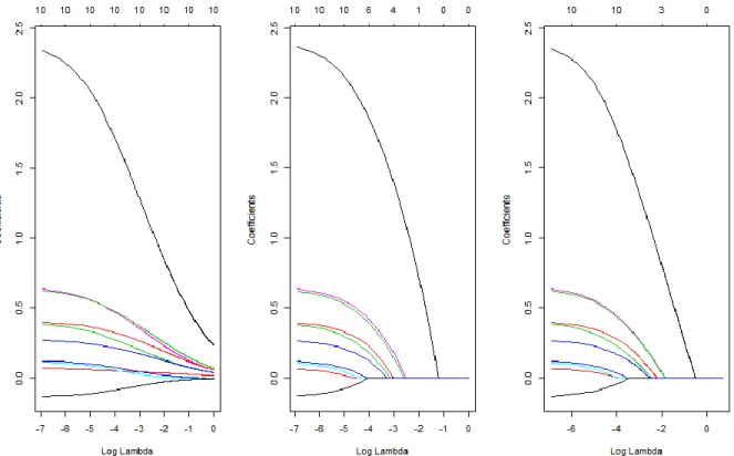
compare the variable selection feature for Ridge, Lasso and Elastic Net, we look the variables trace plots for these three regression approaches on the case 1 data first.

Figure 2. Variable trace plots for Ridge, Lasso and Elastic net for case 1. The left one is for ridge; middle one is the trace plot for lasso; the one on right is Elastic net.

In the plot above, each colored line represents the values of different coefficient, lambda is the tuning parameter tested in the selection procedure. As lambda increases, the coefficients are pulled towards to zero, with less important parameters being pulled to zero earlier. The coefficients of ridge regression could never be zero, when the lambda is big enough, the lasso and elastic net will assign zeros to variables which contribute to model very little. The Elastic net trace plot looks almost identical with the lasso plot, when there is no

(25)

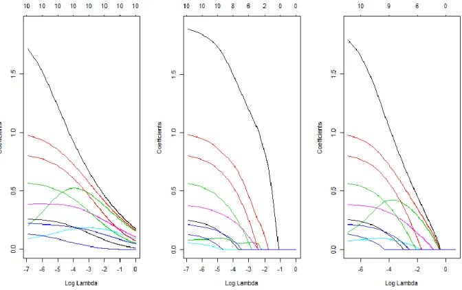
collinearity present in the data, Lasso and Elastic net behave similarly. Now, let us look the trace plots for case 2, where the collinearity problem exists.

Figure 3. Variable trace plots for Ridge, Lasso and Elastic net for case 2. The left one is for ridge; middle one is the trace plot for lasso; the one on right is Elastic net.

Ridge regression solves the collinearity problem by shrinking the coefficients towards to each other. For Lasso, it randomly chooses one from a set of strong but correlated variables, however Elastic net has a compromise solution by keeping all the correlated variables in the model and assigns similar coefficients to these variables. If we compare the model performance on the prediction accuracy by looking the AUC for the validation data, no regression method outperform others substantially for the p<<n cases regardless of the existence of collinearity. AIC, BIC and EBIC are the model fit assessing method with the

(26)

penalty terms on the number of parameters that are selected for the models, similar to the models fitted by regular logistic regression. AIC has a favor to model with more variables, which adequately describe the unknown of the data. BIC has stricter penalty terms on the number of parameters, which tend to select models that are simpler and easier to interpret. EBIC adds one more penalty term to BIC, which considers the complexity of entire model space, however with this new penalty term, EBIC has a favor to models with even fewer variables by scarifying some prediction accuracy. From the simulation results above, we see that the models chosen by EBIC contains the fewest variables for each regression method for case 1. In case 2, BIC and EBIC agree on the models selections, however these models are the simplest models. The pairwise correlated variables groups for the simulation data with collinearity: Correlation=0.95: x1, x4, x5, x6, x7, x8; Correlation=0.75: x3, x9, x10, x11, x12, x13.

Table 3

Model Lambda Number of variables AUC Model Lambda Number of variables AUC Ridge 0.000 100 0.9690 Ridge 0.000 100 0.9608 Lasso 0.047 6 0.9690 Lasso 0.056 8 0.9752 Elastic Net 0.111 6 0.9651 Elastic Net 0.075 16 0.9904

p=100 and n=500 witout collinearity p=100 and n=500 with collinearity

EBIC EBIC

Case 3 Case 4

BIC BIC

(27)

Table 4

Table 5

The ridge regression always keeps all the variables in the model, which results the penalty terms in AIC, BIC and EBIC has no effect on it. So we mainly compare Lasso and

EBIC EBIC

Case 5 Case 6

BIC BIC

AIC AIC

Case 7 Case 8

BIC BIC

AIC AIC

(28)

Elastic Net, which have automated variable selection feature. Similar to what we see for case 1 and case 2, these two regression methods would not outperform to each other substantially for cases 3, 4, 5 and 6 data by comparing the Area under Curve for validation data; in case 3, case 5 and case 7, it turns out that EBIC and BIC agree on the models selection for Lasso and Elastic net regression, Lasso and Elastic net also contains same variables for each information criteria; in case 3 the models contains 5 out of 6 the pre-selected powerful variables: x1, x3, x22, x23, x24; in case 5, the models EBIC chooses the models with 4 variables: x1, x22, x23 and x24; in case 7, the models chosen by EBIC correctly select 2 variables: x22 and x23, BIC selects the model with 3 variables: x1, x22 and x23; For the data without presence of collinearity, EBIC and BIC could effectively identify the dominant variables and both information criteria tend to choose the same model in most cases, the models selected by AIC have more variables as we expected, however with more variables in the model, it does not improve the performance dramatically.

When we look case 4, case 6 and case 8, the simulation data with the existence of collinearity, the number of variables selected by lasso is quite different with Elastic net. For table 6 and 7, regardless of the information criteria, only one of the pairwise correlated variables for each correlation group is chosen for lasso model, however Lasso does not always choose the strongest variable among all the correlated one, it tends to choose one of them randomly and ignore others. Unlike lasso regression, Elastic net has the feature to select group effects, the simulation results in table 6 confirm this: in case 4, the models selected by EBIC and BIC not only contain all the pre-selected important variables but also the variables correlated; in case 6 and case 8, model fitted by Elastic net also contains some of the

(29)

correlated variables. Now let us compare if EBIC has any advantages over BIC on identifying important variables, similar to what we see for the simulation data without collinearity, EBIC and BIC favor to the same models for most of the cases. For the cases EBIC and BIC do not agree to each other, EBIC tends to simpler model.

Table 6

Variables Selection for Lasso and Elastic Net by EBIC (Underline represents correlation 0.75 group; Bold represents correlation 0.95 group.)

Table 7

Variables Selection for Lasso and Elastic Net by BIC. (Underline represents correlation 0.75 group; Bold represents correlation 0.95 group.)

Case 4 Case 6 Case 8 Case 4 Case 6 Case 8

Variables of Lasso models selected by EBIC

x4,x10,x22,x23,x24,x33,x35,x60 x3,x4,x22,x23,x24,x68,x486

x3,x4,x22

Variables of Elastic net models selected by EBIC

x1,x2,x3,x4,x5,x22,x23,x24,x68 x1,x3,x4,x5,x6,x7,x8,x9,x10,x11,x12,x13,x22,x23,x24,x96 x4,x5,x22,x23,x98,x242 Case 4 Case 6 Case 8 Case 4 Case 6 Case 8

Variables of Elastic net models selected by BIC Variables of Lasso models selected by BIC

x1,x2,x3,x4,x5,x22,x23,x24,x46,x68,x486 x4,x5,x22,x23,x98,x242 x1,x3,x4,x5,x6,x7,x8,x9,x10,x11,x12,x13,x22,x23,x24,x96 x1,x3,x20,x22,x23,x24,x33,x35,x60,x68,x79,x82,x96,x98,x242,x486 x3,x4,x22,x23,x24,x68,x486 x3,x5,x22,x23,x98,x242,x1377,x1421

(30)

From the simulation results above, Ridge, Lasso and Elastic net do not outperform each other on prediction accuracy substantially. Ridge regression does not have the automated variable selection feature, it always keeps all the variables in the model with shrinking the coefficients of the less important variables towards to zero. Lasso and Elastic net behave similarly for the data without highly correlated variables, however, when collinearity problem presents in the data, Lasso tends to randomly choose one of the correlated variables, conversely, Elastic net keeps correlated variables in the model. EBIC is a stricter variable selection criteria, which has favor to parsimony model, compare to BIC and AIC. However, EBIC does not perform significantly better than BIC in terms of variable selection, in most cases EBIC and BIC pick the same models.

(31)

Chapter 6: Applications Arcene Data

The data were obtained from The National Cancer Institute, which consist of mass-spectra obtained with the SELDI technique containing the biological information for each patient. The sample has 200 observations including patients with cancer and healthy patients. The purpose of this data is to distinguish cancer versus normal patterns from these massive spectrometric data, to be precise, 10000 features which are all integers ranged from 0 to 700. The task here is to see which approach among Ridge, Lasso and Elastic Net chosen by AIC, BIC and EBIC could successfully identify important variables. Before we fit models on the data, some of the variables which have a lot missing values are removed, we have 9939 variables left. The whole sample is split into train (67% of the data) and validation (33% of the data). In order to test the effect of the normalization of the data, we will build two sets of models: the first set are based on the data with original scale; the other set of models are built on the normalized data.

(32)

Table 8

Model Results for Arcene Data in Original Scale

Table 9

Model Results for Normalized Arcene Data

Variables Model Lambda Number of variables AUC

Ridge 0.000 9939 0.6929 x1-x9939

Lasso 0.248 2 0.6076 x3783,x6594

Elastic Net 0.514 2 0.6151 x3783,x6594

Model Lambda Number of variables AUC

Ridge 0.000 9939 0.6929 x1-x9939

Lasso 0.141 5 0.6449 x1936,x3783,x5982,x6594,x9818

Elastic Net 0.514 2 0.6151 x3783,x6594

Ridge 0.000 9939 0.6929 x1-x9939 Lasso 0.102 12 0.7130 x815,x306,x754,x766,x1748,x1936,x3783,x4684,x6594,x7544,x7891,x9818 Elastic Net 0.514 2 0.6151 x3783,x6594 EBIC BIC AIC Variables Model Lambda Number of variables AUC

Ridge 0.000 9939 0.6929 x1-x9939

Lasso 0.127 5 0.6392 x1936,x3783,x5982,x6594,x9818

Elastic Net 0.477 2 0.6285 x3783,x6594

Ridge 0.000 9939 0.6929 x1-x9939

Lasso 0.127 5 0.6392 x1936,x3783,x5982,x6594,x9818

Elastic Net 0.477 2 0.6285 x3783,x6594

Ridge 0.000 9939 0.6929 x1-x9939 Lasso 0.087 12 0.7115 x815,x306,x754,x766,x1748,x1936,x378+E2x4684,x6594,x7544,x7891,x9818 Elastic Net 0.477 2 0.6285 x3783,x6594 EBIC BIC AIC

(33)

Normalization does not change the model results dramatically, dominant variables could always be picked out. The model results of the standardized data is very close to the results on the original data. Like what we observed for the simulation data, Ridge contains all variables in the model, it is not surprising the model fitted by Ridge perform fairly well for both data sets. However keeping all the variables in the model makes the model nearly impossible to interpret. For Elastic net, all three information selection criteria pick the same model with two variables (x3783 and x6594) in both cases, the AUC for the validation data for these three models are not excellent but acceptable. If we compare this model with the model fitted by Lasso under EBIC with same variables, Elastic net model perform slightly better. The best model in terms of AUC for validation data is the one fitted by Lasso under AIC, this model also contains the most variables. Lasso model picked by BIC has 5 variables, however the AUC is not as good as the model chosen by AIC.

Retention Data

Retention project is led by Dr.Robinson in St. Cloud State University, which intends to research students’ academic information and understand the important variables that have strong relationship with the success of students. By analyzing students’ historical patterns, the school wants to improve the ability of predicting which student is at high risk of dropping school and make necessary intervention to ensure students’ academic success based on the needs of students. For this project, Identifying important variables and building model with high prediction accuracy are equally important. We will use the academic data of fall 2010 cohort to build Ridge, Lasso and Elastic Net model to predict if the student will return to school at their third term, and try to select the optimal predicting model that easy to interpret.

(34)

Exploratory Data Analysis

The data contains 4047 observations, 2₃of the data is used to build the model, and the rest of the data serves as validation purpose. Forty-seven variables will be used to build the models including 25 nominal variables and 22 continuous variables:

Table 10

Distributions of Nominal Variables of Retention Data

1 0 1 0 ACE 22% 78% 28% 72% 0.0002 Honors 7% 93% 2% 98% 0.0000 Dist1 96% 4% 95% 5% 0.0203 Female 54% 46% 52% 48% 0.3585 International 97% 3% 98% 2% 0.0107 StudentOfColor1 11% 89% 12% 88% 0.8810 FirstGeneration1 13% 87% 14% 86% 0.5627 HS_GPA1 97% 3% 97% 3% 0.7985 HS_Rank1 81% 19% 65% 35% 0.0000 HS_Pct1 89% 11% 89% 11% 0.7084 HS_MnSCU_Region7 31% 69% 28% 72% 0.0329 HS_MnSCU_Region11 33% 67% 33% 67% 0.8257 HS_MnSCU_Region_OutofState 10% 90% 14% 86% 0.0011 HS_MnSCU_Region_Unknown 5% 95% 4% 96% 0.1070 ACT1 97% 3% 96% 4% 0.0054 ACT_Math1 97% 3% 94% 6% 0.0001 ACT_English1 97% 3% 94% 6% 0.0001 ACT_Reading1 97% 3% 94% 6% 0.0001 ACT_Science1 97% 3% 94% 6% 0.0000 GrantFlag1 45% 55% 43% 57% 0.1442 ScholarshipFlag1 31% 69% 23% 77% 0.0000 LoanFlag1 66% 34% 73% 27% 0.0001 WorkStudyFlag1 12% 88% 12% 88% 0.9796 EFC_Total1 74% 26% 75% 25% 0.4829 1st_Term_On_Campus1 77% 23% 75% 25% 0.2111

Variable P-value of chi square test

3rd term retention

(35)

Table 10 above shows the distribution of nominal variables that we will use in the model. Dist1 is a missing value indicates for students who do not have an address in file. ACT1, ACT_Math1, ACT_English1, ACT_Reading1, ACT_science1, GrantFlag1, LoanFlag1, WorkStudyFlag1 and EFC_Total1 serve the same role as missing value indicators here. The variables in table 10 above shows the variables with small P-value of Chi-square test between the nominal variable and the dependent variables, the small P-values indicate these variables have potential to play an important role for the predicting modeling.

Table 11 below shows the descriptive statistics of all the continuous variables, we also conduct the T test to compare if each explanatory variable in each level is significantly different. The variables with small P-values could be important in the model we will build.

(36)

Table 11

Distributions of Continuous Variables of Retention Data

We keep ACT composite score and all the ACT subjects’ scores in the model, which are highly correlated. We expect Elastic net could select the group effects, and we also want to test how Lasso and Ridge handle the collinearity.

3rd Term Retention Variable N Min First quantileMedian Mean Std DevThird Quantile Max P-value of T test 1 1st_Term_TermAttemptedCreditsUgrad 3055 3 14 15 14.53 1.42 16 18 0 1st_Term_TermAttemptedCreditsUgrad 1232 1 13 14 14.28 1.6 15 20 1 1st_Term_TermCompletedCreditsUgrad 3055 0 13 14 13.77 2.33 15 18 0 1st_Term_TermCompletedCreditsUgrad 1232 0 7 12 10.31 5.07 14 20 1 1st_Term_TermGPAUgrad 3055 0 2.37 2.91 2.82 0.73 3.36 4 0 1st_Term_TermGPAUgrad 1232 0 1 2.07 1.96 1.18 2.97 4 1 ACT_English2 3055 0 17 20 19.99 5.66 23 36 0 ACT_English2 1232 0 16 20 19.2 6.49 23 35 1 ACT_Math2 3055 0 18 22 21.14 5.5 24 35 0 ACT_Math2 1232 0 17 21 20.02 6.34 24 34 1 ACT_Reading2 3055 0 18 22 21.14 5.5 24 35 0 ACT_Reading2 1232 0 17 21 20.02 6.34 24 34 1 ACT_Science2 3055 0 20 22 21.25 5.17 24 35 0 ACT_Science2 1232 0 19 21 20.41 6.29 24 35 1 ACT2 3055 0 19 21 21 4.93 24 35 0 ACT2 1232 0 18 21 20.34 5.69 24 33 1 Age 3055 16 18 18 18.13 0.44 18 20 0 Age 1231 16 18 18 18.16 0.49 18 20 1 AppDaysBeforeTerm 3055 -4 181 244 227.21 76.1 285 417 0 AppDaysBeforeTerm 1232 -2 153 223 207.05 81.63 265 417 1 Dist2 3055 0 21.8 48.2 56.86 52.3 72.09 251 0 Dist2 1232 0 24.5 50.7 60.07 52.76 74.59 251 1 EFC_Total2 3055 0 0 6119 11667.96 15845.72 17178 215272 0 EFC_Total2 1232 0 10 6232 11997.03 21885.55 16316.25 322989 1 GrantFlag2 3055 0 0 0 1222.84 1606.49 2735.6 7184.22 0 GrantFlag2 1232 0 0 0 1113.83 1549.96 2525 7413 1 HS_GPA2 3055 0 2.87 3.23 3.12 0.74 3.57 4.76 0 HS_GPA2 1232 0 2.71 3 2.94 0.69 3.34 4.17 1 HS_Pct2 3055 0 37.5 56.58 53.33 27.32 74.64 99.81 0 HS_Pct2 1232 0 31.28 48.19 46.2 25.05 63.53 98.71 1 HS_Rank2 3055 0 11 64 101.94 114.28 154 702 0 HS_Rank2 1232 0 0 45 91.46 118.84 137 739 1 LoanFlag2 3055 0 0 2750 2713.1 2587.39 4750 11518 0 LoanFlag2 1232 0 0 2750 3021.98 2578.51 4750 11811 1 ScholarshipFlag2 3055 0 0 0 347.03 748.44 500 6376 0 ScholarshipFlag2 1232 0 0 0 230.04 624.06 0 5738 1 TransferCredits2 3055 0 0 0 5.4 10.17 7 71 0 TransferCredits2 1232 0 0 0 3.67 8.62 3 71 1 TransferGPA2 3055 0 0 0 0.87 1.41 2.15 4 0 TransferGPA2 1232 0 0 0 0.58 1.19 0 4 1 WorkStudyFlag2 3055 0 0 0 161.15 454.95 0 2250 0 WorkStudyFlag2 1232 0 0 0 161.88 455.94 0 1590 0.63160 0.00000 0.00000 0.00000 0.00019 0.00000 0.00000 0.00003 0.00036 0.06208 0.00000 0.07079 0.00000 0.00000 0.96214 0.03927 0.00000 0.00000 0.00828 0.00040 0.00000

(37)

Table 12

Correlation Matrix for ACT Scores

Model Results

Model results shown below, the logistic model was selected by stepwise procedure. If we look at the AUC for the validation data, all the models selected by different information criteria perform similarly to each other. EBIC and BIC choose the same model for each regression method. Elastic net models chosen by EBIC and BIC has the least number of variables, which contains all the variables that also present in all other models. We also run the models on the standardized retention data, we have the same results, which means normalization does not have great impact on the model fitting.

ACT2 ACT_Math2 Act_English2 ACT_Reading2 ACT_Science2

ACT2 1.0000 0.8512 0.8808 0.8512 0.8640

ACT_Math2 0.8512 1.0000 0.7640 1.0000 0.8365

Act_English2 0.8808 0.7640 1.0000 0.7640 0.7860 ACT_Reading2 0.8512 1.0000 0.7640 1.0000 0.8365 ACT_Science2 0.8648 0.8365 0.7860 0.8365 1.0000

(38)

Table 13

Model Results for Retention Data

Logistic N/A 8 0.7642

Ridge 0.001 47 0.7583

Lasso 0.021 6 0.7562

Elastic Net 0.045 5 0.7533

Logistic N/A 8 0.7642

Ridge 0.001 47 0.7583

Lasso 0.021 6 0.7562

Elastic Net 0.011 5 0.7533

Logistc N/A 20 0.7653 Ridge 0.001 47 0.7583 Lasso 0.002 36 0.7653 Elastic Net 0.004 37 0.7662 EBIC BIC AIC

(39)

Table 14

Variables Selection for Retention Data

Logistic Ridge Lasso Elastic Net Logistic Ridge Lasso Elastic Net Logistic Ridge Lasso Elastic Net

ACE1 X X X X X Honors1 X X X X X X AppDaysBeforeTerm X X X Dist1 X X X Dist2 X X X X X Female X X X X X X Age X X X X X X US Citizen X X X X X StudentOfColor1 X X X X X X X X X FirstGeneration1 X X X X X Veteran1 X X X HS_GPA1 X X X X X X HS_GPA2 X X X X HS_Rank1 X X X X X X X X X X X X HS_Rank2 X X X X X X HS_Pct1 X X X X X X X X X X X X HS_Pct2 X X X X X X HS_MnSCU_Region7 X X X X X X HS_MnSCU_Region11 X X X X X X HS_MnSCU_Region_OutofState X X X X X X X X X X X X HS_MnSCU_Region_Unknown X X X X X ACT1 X X X X ACT2 X X X X X ACT_Math1 X X X ACT_Math2 X X X ACT_English1 X X X ACT_English2 X X X X X ACT_Reading1 X X X ACT_Reading2 X X X ACT_Science1 X X X X X X X X ACT_Science2 X X X X X X TransferCredits2 X X X X X TransferGPA2 X X X X X GrantFlag1 X X X X X GrantFlag2 X X X X X ScholarshipFlag1 X X X X X ScholarshipFlag2 X X X LoanFlag1 X X X X X LoanFlag2 X X X WorkStudyFlag1 X X X X X WorkStudyFlag2 X X X X X EFC_Total1 X X X X X EFC_Total2 X X X X X 1st_Term_On_Campus1 X X X X X X X X 1st_Term_TermAttemptedCreditsUgrad X X X X X X X X 1st_Term_TermCompletedCreditsUgrad X X X X X X X X X X 1st_Term_TermGPAUgrad X X X X X X X X X X

(40)

Chapter 7: Discussion

Our results from the simulation data show thatRidge, Lasso and Elastic net regression methods behave similarly to each other in terms of prediction accuracy. However, Lasso and Elastic net have substantial advantages over Ridge on variable selection; with the L1 regularization involved, Lasso and Elastic net tends to penalize the absolute size of the coefficients to zero, the larger the penalty applied, the further estimates are shrunk towards to zero. As the amount of shrinkage increase, the coefficients of less important variables reach zero first, which gives Lasso and Elastic net the feature of automatic feature selection and also yield a sparse model containing only a subset of the variables in the full model. As a result, the models generated from Lasso and Elastic net are much easier to interpret. Elastic net perform closely to Lasso regression on both prediction accuracy and variable selection, if there is no collinearity in the data. However if multi-collinearity present in the data, Elastic net will select group effects, in other words, it will keep the all the variables correlated to each other in model if all of contribute to the model significantly, Lasso tends to randomly select one of them. Ridge regression does not have the function of variable selection, no matter how big the shrinkage factor is, Ridge keeps all the variables in the model, it only shrinks the coefficients of less important variables very close to zero but will never be zero, because of the difficulties of variable selection and model interpretation, Ridge regression is not always the first choice compared to Lasso and Elastic net regression.

From the modeling fitting results of simulation data and two applications, EBIC does not hold outstanding advantages over BIC on model selection; EBIC tends to select a simple model by scarifying the prediction accuracy, which also means EBIC rules some important

(41)

variables out and only keep the most dominant variables to make the model simpler. BIC has a penalty term on the number of parameters which is stricter than the terms of AIC, which leads to the simpler model favored by BIC. The simulation results shows the similar principles, AIC often risks choosing models with more variables. However for the most of the simulation results, the models with more variables chosen by AIC perform slightly better than others. If the primary goal is to select a model with high prediction accuracy, AIC is a better choice over EBIC and BIC; if the primary goal is to find important factors, BIC is a more reliable information criteria over AIC and EBIC, since BIC could effectively identify the important variables, and EBIC favors too small a model which risks ruling some important variables out. In the cases that a small set of variables are prominent, the variable selection outcomes between EBIC and BIC are very close, we observe this in case 7 and case 8 of the simulation data and the results of Arcene data. When there is no dominant variables existing in the data, EBIC would outperform BIC and it could effectively identify important variables, this conclusion is supported by the simulation results in Chen and Chen’s original study (Chen & Chen, 2012).

One thing we did not consider in the simulation study is the impact of the possible variations in the explanatory variables since all the data were generated from standard normal. However, in the real data analysis, we did consider standardizing the explanatory variables first such that each has mean of 0 and standard deviation of 1 and then fitted the models. We found that there was no obvious evidence of the normalizing effect. The standardized Retention data and the data on original scale share the same model fitting results. The only big difference we observed on the standardized Arcene data is that the model selected by EBIC

(42)

contains 5 variables instead of 2, and as a result, EBIC and BIC agree on the variable selection.

There are some other regularization methods developed, these approaches are not in the scope of this paper, we will mention a few of them: Adaptive lasso is proposed by Hui Zou (2006), which is developed by assign adaptive weighted coefficients to L1 penalty, in Zou’s Paper, the simulation results of Adaptive Lasso shows the advantage of computation efficiency over regular Lasso and estimates parameters consistently. SCAD is a variable selection method developed by Fan and Li (Fan & Li, 2001), which sets a boundary for the penalty function as a result of reducing bias. It would be interesting to include them in the comparison in the future.

(43)

References

Akaike, H. (1973). Information theory and an extension of the maximum likelihood principle. Proceedings of the 2nd International Symposium on Information Theory, pp. 257-281. Chen, J., & Chen, Z. (2008). Extended Bayesian information criteria for model selection with

large model spaces. Biometrika, 95(3), 759-771.

Chen, J., & Chen, Z. (2012). Extended BIC for small-n-large-p sparse GLM. Statistica Sinica, 22, 555-574.

Fan, J., & Li, R. (2001). Variable selection via non-concave penalized likelihood and its oracle properties. Journal of American Statistical Association, 96, 1348-1356.

Ghosh, J., Delampady, M., & Samanta, T. (2006). An introduction to Bayesian analysis: Theory and methods. Springer Science and Business Media, LLC.

Horel, A., & Kennard, R. (1970). Ridge regression: Biased estimation for nonorthogonal problems. Technometrics, 12(1), 55-67.

Siegmund, D. (2004). Model selection in irregular problems: Applications to mapping quantitative trait loci. Biomertrika, 91, 785-800.

Tibshirani, R. (1996). Regression shrinkage and selection via the Lasso. Journal of the Royal Statistical Society, 58(1), 267-288.

Wahba, G., Golub, G., & Heath, M. (1979, May). Generalized cross-validation as a method for choosing a good ridge parameter. Technometric, 21(2).

Zou, H. (2006). The adaptive lasso and its oracle properties, Journal of the American Statistical Association, 101, 1418-1429.

(44)

Zou, H., & Hastie, T. (2005). Regularization and variable selection via the elastic net. Journal of the Royal Statistical Society, 67, 301-332.

(45)

Appendix A

Variable Definitions for Retention Data

ACE: Academic Collegiate Excellence (ACE) program is designed to help students who did not meet the admission requirements but have potential to be successful students. We will use this as one of the variable in the model, if the student is in ACE

program, then ACE=1, otherwise, ACE=0.

Honors: The University Honors Program provides supportive and challenging learning environment for determined students to enhance the skills in analysis, synthesis and interpersonal communication, students admitted into this program have an outstanding academic background.

Female: This is the gender indictor, where 1 represents female and 0 is male. International: A variable that tells which student is an international student. StudentOfColor1: This dummy variable tells which student is not white.

Firstgeneration1: An indicator tells whether this student is the first college student in the family.

HS_MNSCU_region7, HS_MNSCU_Region11,

HS_MNSCU_Region_outofstate, HS_MNSCU_Region_unknown :

These four variables indicate the location of the high schools of students.

1st_term_on_Campus1: If the students live on campus for the 1st semester, the assign 1 to this variable, otherwise 0.

(46)

Appendix B R Code

Case1:

########simulation data with 10 variables and 1000 observations. set.seed(12345679) x1=rnorm(500) x2=rnorm(500) x3=rnorm(500) x4=rnorm(500) x5=rnorm(500) x6=rnorm(500) x7=rnorm(500) x8=rnorm(500) x9=rnorm(500) x10=rnorm(500)

########simulate the coefficients of the variables; set.seed(12345679)

b1=10*runif(1) b2=runif(1) b3=runif(1) b4=runif(1)

(47)

b5=runif(1) b6=runif(1) b7=runif(1) b8=runif(1) b9=runif(1) b10=runif(1) #####create function z=runif(1)+b1*x1+ b2*x2+ b3*x3+ b4*x4+ b5*x5+ b6*x6+ b7*x7+ b8*x8+ b9*x9+ b10*x10

######create reverse logit link function pr = 1/(1+exp(-z))

y = rbinom(500,1,pr) ######create the dataset

(48)

train=data.frame(x1=x1, x2=x2, x3=x3, x4=x4, x5=x5, x6=x6, x7=x7, x8=x8, x9=x9, x10=x10,y)

#####create train and validation library(caTools) sample1=sample.split(train$y,SplitRatio=2/3) train1=train[sample1,] validation=train[!sample1,] t.y=data.matrix(train1$y) t.x=data.matrix(train1[,1:10]) v.y=data.matrix(validation$y) v.x=data.matrix(validation[,1:10]) Case 2:

(49)

########simulation data with 10 variables and 1000 observations. set.seed(12345679) x1=rnorm(500) x2=jitter(x1,factor=2500) x3=jitter(x2,factor=2500) x4=rnorm(500) x5=jitter(x1,factor=7500) x6=jitter(x1,factor=7500) x7=rnorm(500) x8=rnorm(500) x9=rnorm(500) x10=rnorm(500)

########simulate the coefficients of the variables; set.seed(12345679) b1=3*runif(1) b2=runif(1) b3=runif(1) b4=runif(1) b5=runif(1) b6=runif(1) b7=runif(1)

(50)

b8=runif(1) b9=runif(1) b10=runif(1) #####create function z z=runif(1)+b1*x1+ b2*x2+ b3*x3+ b4*x4+ b5*x5+ b6*x6+ b7*x7+ b8*x8+ b9*x9+ b10*x10

y = rbinom(500,1,pr)

######create the dataset train=data.frame(x1=x1,

(51)

x2=x2, x3=x3, x4=x4, x5=x5, x6=x6, x7=x7, x8=x8, x9=x9, x10=x10,y=y)

#####create train and validation library(caTools) sample1=sample.split(train$y,SplitRatio=2/3) train1=train[sample1,] validation=train[!sample1,] t.y=data.matrix(train1$y) t.x=data.matrix(train1[,1:10]) v.y=data.matrix(validation$y) v.x=data.matrix(validation[,1:10])

(52)

Case 3:

########simulation data with 10 variables and 1000 observations. set.seed(12345679) x1=rnorm(500) x2=rnorm(500) x3=rnorm(500) x4=rnorm(500) x5=rnorm(500) x6=rnorm(500) x7=rnorm(500) x8=rnorm(500) x9=rnorm(500) x10=rnorm(500) x11=rnorm(500) x12=rnorm(500) x13=rnorm(500) x14=rnorm(500) x15=rnorm(500) x16=rnorm(500) x17=rnorm(500) x18=rnorm(500) x19=rnorm(500)

(53)

x20=rnorm(500) x21=rnorm(500) x22=rnorm(500) x23=rnorm(500) x24=rnorm(500) x25=rnorm(500) x26=rnorm(500) x27=rnorm(500) x28=rnorm(500) x29=rnorm(500) x30=rnorm(500) x31=rnorm(500) x32=rnorm(500) x33=rnorm(500) x34=rnorm(500) x35=rnorm(500) x36=rnorm(500) x37=rnorm(500) x38=rnorm(500) x39=rnorm(500) x40=rnorm(500) x41=rnorm(500)

(54)

(55)

(56)

x86=rnorm(500) x87=rnorm(500) x88=rnorm(500) x89=rnorm(500) x90=rnorm(500) x91=rnorm(500) x92=rnorm(500) x93=rnorm(500) x94=rnorm(500) x95=rnorm(500) x96=rnorm(500) x97=rnorm(500) x98=rnorm(500) x99=rnorm(500) x100=rnorm(500)

########simulate the coefficients of the variables; set.seed(12345679)

b1=10*runif(1) b2=10*runif(1) b3=10*runif(1) b4=runif(1)

(57)

b5=runif(1) b6=runif(1) b7=runif(1) b8=runif(1) b9=runif(1) b10=runif(1) b11=runif(1) b12=runif(1) b13=runif(1) b14=runif(1) b15=runif(1) b16=runif(1) b17=runif(1) b18=runif(1) b19=runif(1) b20=runif(1) b21=runif(1) b22=10*runif(1) b23=10*runif(1) b24=10*runif(1) b25=runif(1) b26=runif(1)

(58)

b27=runif(1) b28=runif(1) b29=runif(1) b30=runif(1) b31=runif(1) b32=runif(1) b33=runif(1) b34=runif(1) b35=runif(1) b36=runif(1) b37=runif(1) b38=runif(1) b39=runif(1) b40=runif(1) b41=runif(1) b42=runif(1) b43=runif(1) b44=runif(1) b45=runif(1) b46=runif(1) b47=runif(1) b48=runif(1)

(59)

(60)

(61)

b93=runif(1) b94=runif(1) b95=runif(1) b96=runif(1) b97=runif(1) b98=runif(1) b99=runif(1) b100=runif(1) #####create function z set.seed(12345679) z=runif(1)+b1*x1+ b2*x2+ b3*x3+ b4*x4+ b5*x5+ b6*x6+ b7*x7+ b8*x8+ b9*x9+ b10*x10+ b11*x11+

(62)

b12*x12+ b13*x13+ b14*x14+ b15*x15+ b16*x16+ b17*x17+ b18*x18+ b19*x19+ b20*x20+ b21*x21+ b22*x22+ b23*x23+ b24*x24+ b25*x25+ b26*x26+ b27*x27+ b28*x28+ b29*x29+ b30*x30+ b31*x31+ b32*x32+ b33*x33+

(63)

(64)

(65)

b78*x78+ b79*x79+ b80*x80+ b81*x81+ b82*x82+ b83*x83+ b84*x84+ b85*x85+ b86*x86+ b87*x87+ b88*x88+ b89*x89+ b90*x90+ b91*x91+ b92*x92+ b93*x93+ b94*x94+ b95*x95+ b96*x96+ b97*x97+ b98*x98+

(66)

(67)

b99*x99+ b100*x100

y = rbinom(500,1,pr)

######create the dataset train=data.frame(x1=x1, x2=x2, x3=x3, x4=x4, x5=x5, x6=x6, x7=x7, x8=x8, x9=x9, x10=x10, x11=x11, x12=x12,

(68)

x13=x13, x14=x14, x15=x15, x16=x16, x17=x17, x18=x18, x19=x19, x20=x20, x21=x21, x22=x22, x23=x23, x24=x24, x25=x25, x26=x26, x27=x27, x28=x28, x29=x29, x30=x30, x31=x31, x32=x32, x33=x33, x34=x34,

(69)

(70)

(71)

x79=x79, x80=x80, x81=x81, x82=x82, x83=x83, x84=x84, x85=x85, x86=x86, x87=x87, x88=x88, x89=x89, x90=x90, x91=x91, x92=x92, x93=x93, x94=x94, x95=x95, x96=x96, x97=x97, x98=x98, x99=x99, x100=x100,y=y)

(72)

#####create train and validation library(caTools) sample1=sample.split(train$y,SplitRatio=2/3) train1=train[sample1,] validation=train[!sample1,] t.y=data.matrix(train1$y) t.x=data.matrix(train1[,1:100]) v.y=data.matrix(validation$y) v.x=data.matrix(validation[,1:100]) Case 4:

########simulation data with 10 variables and 1000 observations. set.seed(12345679) x1=rnorm(500) x2=rnorm(500) x3=rnorm(500) x4=jitter(x1,factor=2500) x5=jitter(x1,factor=2500) x6=jitter(x1,factor=2500) x7=jitter(x1,factor=2500) x8=jitter(x1,factor=2500) x9=jitter(x3,factor=7500)