Bayesian Analysis of Dynamic Multivariate Models with Multiple Structural Breaks

Title

Bayesian Analysis of Dynamic Multivariate Models

with Multiple Structural Breaks

Author(s)

Sugita, Katsuhiro

Citation

Issue Date

2006-11

Type

Technical Report

Text Version

URL

http://hdl.handle.net/10086/16988

Right

#2006-14

Discuttion Paper #2006-14

Bayesian Analysis of Dynamic Multivariate Models

with Multiple Structural Breaks

by

Bayesian Analysis of Dynamic Multivariate Models with

Multiple Structural Breaks

Katsuhiro Sugita∗

Graduate School of Economics, Hitotsubashi University, Tokyo 186-8601, Japan

Abstract

This paper considers a vector autoregressive model or a vector error correction model with multiple structural breaks in any subset of parameters, using a Bayesian approach with Markov chain Monte Carlo simulation technique. The number of structural breaks is deter-mined as a sort of model selection by the posterior odds. For a cointegrated model, cointe-grating rank is also allowed to change with breaks. Bayesian approach by Strachan (Jour-nal of Business and Economic Statistics 21 (2003) 185) and Strachan and Inder (Jour(Jour-nal of Econometrics 123 (2004) 307) are applied to estimate the cointegrating vectors. As empirical examples, we investigate structural changes in the predictive power of the yield curve and the US term structure of interest rates. We find strong evidence of three structural changes in both applications.

Key words: Bayesian inference; Structural break; Cointegration; Bayes factor; JEL classification: C11; C12; C32

1

Introduction

The last decade has seen extensive study of the structural break in time series models. Papers such as Perron (1989) deals with this issue in the framework of a priori imposed break dates, ∗ _{Graduate School of Economics, Hitotsubashi University, 2-1 Naka, Kunitachi, Tokyo 186-8601, Japan. Tel.:}

while others use methods where the break date is endogenized (Banerjee, Lumsdaine and Stock, 1992; Christiano, 1992; and Zivot and Andrews, 1992). Much of the subsequent research focus on testing for a structural break when the break date may not be known. Among these, the supF statistic of Andrews (1993) and the expF and aveF statistics of Andrews-Ploberger (1994) are most notable. Based on Andrews and Andrews-Ploberger’s statistics, Hansen (2000) proposes a bootstrapping method for testing for a single structural break.

An extension of the literature on testing for a structural break involves allowing for more than one possible break date. For many macroeconomic or financial time series with the possibility of a structural break, the assumption of at most one break date is unrealistic and restrictive. Bai and Perron (1998) propose a test for multiple structural breaks at unknown dates using the dou-ble maximum test. Another testing method for detecting multiple changes is a likelihood ratio test with the null of l breaks against the alternative l+1 break points (Bai, 1999). While these methods only allow for structural breaks in mean, breaks in variance are often found in economic and financial data. Schwert (1990) finds that volatility of the stock-market is higher during and after the 1987 crash. Inclan (1993), Inclan and Tiao (1994), and Chen and Gupta (1997) detect multiple breaks in variance for several series of stock returns. Engel and Hakkio (1996) find that European Monetary System exchange rates have higher volatility during the periods of alignment, and Kim and Engel (1999) find multiple breaks in variance in real exchange rates associated with historically significant monetary events. Kim and Nelson (1999) combine a structural break with the Markov switching model to find evidence of variance breaks in postwar business cycles. For a Bayesian approach to multiple structural breaks, Wang and Zivot (2000) consider univariate models with multiple breaks in level, trend and variance. Another Bayesian approach to multiple structural breaks is provided by Chib (1998), who considers structural breaks as regime switching of discrete-state Markov process with restricted transition probabilities.

The above literatures consider structural break(s) in univariate models. The estimation of and testing for structural break in cointegrated models has been also received attention. Gregory and Hansen (1996a) study residual-based tests for cointegration with a single structural break in a single equation model. They proposed ADF−, Zα−, and Zt−type tests designed to test the null of no cointegration against the alternative of cointegration in the presence of a possible regime shift.

Gregory and Hansen (1996b) extend this work, by permitting a trend shift as well as a regime shift and providing the critical values for testing cointegration with a single break. Seo (1998) derives the Lagrange multiplier test for structural breaks in cointegration relations and adjustment terms, using the framework of Andrews and Ploberger (1994). Hansen and Johansen (1999) test parameter instability in cointegrating vectors based on Nyblom’s L statistic (1989). Hansen (2003) explores the multiple-break case in cointegrated systems, and allows changes in any subset of the parameters, where the time of the change points and the number of cointegration relations are treated as known. Inoue (1999) derives a rank test for cointegrated systems with a structural change in trend. Bai et al. (1998) develop methods for constructing confidence intervals for the date of a single break in multivariate time series, and show that the accuracy of the break point estimators can be improved with series that have common breaks. While these authors assume the constant volatility in VAR, Bai (2000) allows the variance-covariance matrices to be affected by the breaks, using the quasi-maximum likelihood method. He also considered multiple breaks instead of a single break.

The main contribution of this paper is the development of general multivariate structural break models. We consider multiple structural breaks in any subset of the parameters in VAR or co-integrated VAR models, using a Bayesian approach which extends Wang and Zivot’s (2000) method for detecting multiple structural changes in univariate models. In cointegration analysis, as changes in volatility and other terms are likely to affect the strength of the adjustment toward the equilibrium, it is of interest to analyze a model where structural breaks also affect in the ad-justment terms, cointegrating vectors, and/or cointegrating rank. Hansen (2003) considers similar general cointegration models with structural breaks in any subset of parameters, where the number of cointegration relations, the number of breaks and the location of the break points are known. This paper considers general multivariate cointegrated models with breaks in any subset of the parameters where the break points and the rank are unknown. This is possible by applying a valid Bayesian approach to cointegration proposed by Strachan (2003), which is based on the singular value decomposition method by Kleibergen and Paap (2002) and Kleibergen and van Dijk (1998). For a less general case where cointegrating rank is not allowed to change with breaks, a simpler method by Strachan and Inder (2004) can be applied.

The Bayesian approach has several advantages over the classical method in the context of structural break models as it is technically simpler, allows inferences that are optimal given the framework, and allows for nonnested model comparison by computing posterior odds (see Raftery, 1994). Additionally, inference from the Bayesian approach is based on the exact finite sample properties for all of the parameters of the model. Finally, unlike most classical methods for de-tecting structural breaks, the Bayesian approach provides information about uncertainty in all estimated parameters including the location of the break dates. When the posterior probability mass function of the change point exhibits a substantial range in dates, the structural break may occur smoothly, rather than suddenly at a particular date.

This paper is organized as follows. Section 2 presents a Bayesian approach to VAR model with multiple structural breaks, using a simple Gibbs sampler. In Section 3, we extend the approach of the VAR model with multiple breaks to vector error correction models with multiple breaks in deterministic terms, adjustment term, cointegrating vector, variance-covariance matrices, and cointegrating rank, using Metropolis-within-Gibbs sampling algorithm, based on the method by Strachan (2003). We also consider a case where cointegrating rank is not allowed to change with breaks. This case is treated by applying a simpler method by Strachan and Inder (2004) with the Griddy-Gibbs sampler to estimate the cointegrating vectors. Section 4 considers the issue of model selection for detecting multiple structural breaks using Bayes factors calculated by using Schwarz BIC method and Chib’s (1995) method. In Section 5 determining the cointegrating rank is considered for the two cases - one for where the cointegrating rank is subject to change and the other is for where it is not subject to change with breaks. In Section 7, Monte Carlo simulations are presented using artificially generated data for VAR models and vector error correction models with multiple breaks in order to examine the performances of detecting the number of breaks using our methods. To illustrate an empirical study of the VAR model with multiple breaks, Section 8 presents the predictive power of the yield curve on output growth. For an application of the vector error correction model with multiple breaks, we apply the method to investigate US term structure of interest rates. Section 9 concludes. All computation in this paper are performed using code written by the author with Ox v3.30 for Linux (Doornik, 1998).

2

Bayesian Inference in Vector Autoregressive Model with Multiple

Structural Breaks

2.1 Statistical Model for VAR with Multiple Structural Breaks

In this section we consider a Bayesian approach to VAR model with multiple structural breaks. Let ytdenote a vector of n-dimensional(1×n)time series. If all parameters in a VAR are assumed to be subject to structural breaks, then the model is

yt =µt+tδt+ p

∑

i=1

yt−iΦt,i+εt (1) where t=p,p+1, . . . ,T ; p is the number of lags; andεt are assumed N(0,Ωt)and independent over time. Dimensions of matrices are µt,δt andεt (1×n),Φt,i andΩt (n×n). The parameters

µt,δt andΩtare assumed to be subject to m structural breaks (m<t) with break points b1, . . . ,bm, where b1<b2<· · ·<bm, so that the observations can be separated into m+1 regimes.

Equation (1) can be rewritten in the matrix format as:

Y =X B+E (2) where Y = y0_p y0_p+1, . . . , y0_T 0 , X = X1 X2 , X1=          s1,p · · · sm+1,p s1,p · · · sm+1,p s1,p+1 · · · sm+1,p+1 2s1,p+1 · · · 2sm+1,p+1 .. . ... ... ... ... · · · s1,T · · · sm+1,T (T−p+1)s1,T · · · (T−p+1)sm+1,T          , X2=          s1,py0p−1 · · · s1,py01 · · · sm+1,py0p−1 · · · sm+1,py01 s1,p+1y0p · · · s1,p+1y0₂ · · · sm+1,p+1y0p · · · sm+1,p+1y0₂ .. . ... ... ... ... ... ... s1,Ty0T−1 · · · s1,Ty0T−p+1 · · · sm+1,Ty0T−1 · · · sm+1,Ty0T−p+1          , B= µ0₁, . . . , µ0_m+1 δ₁0, . . . , δ0_m+1 Φ0_1,1, . . . , Φ0_p,1, . . . , Φ0_1,m+1, . . . , Φ0_p,m+1 0

Let τ be the number of rows of Y (τ×n), so that τ=T−p+1, then X is τ×κ where κ= (np+2)(m+1), and B isκ×n. si,t in X1 and X2 is an indicator variable which equals to 1 if

regime is i and 0 otherwise.

2.2 Prior Distributions and Likelihood Functions for VAR with Multiple Structural

Breaks

Let b= (b1,b2, . . . ,bm)0denote the vector of break dates. We specify priors for parameters, assum-ing prior independence between b, B andΩi, i=1,2, . . . ,m+1, such that p(b,B,Ω1,Ω2, . . . ,Ωm+1) =

p(b)p(B)∏m_i=+₁1p(Ωi). This is because if we consider that the prior for B is conditional onΩas is often used in regression models with the natural conjugate priors, it is not convenient to consider a case when the error covariance is also subject to structural breaks. Thus, the prior density for B is set as the marginal distribution and vectorized as vec(B)unconditional onΩifor convenience. The prior for the covariance-variance matrix,Ωi, is specified with an inverted Wishart density. For the prior for the location of the break dates b, we choose a diffuse prior such that the prior is discrete uniform over all ordered subsequences of t=p+1, . . . ,T−1. We consider that all priors for b,

Ωi, and vec(B)are proper as:

p(b)∼

U

(p+1,T−1) (3)

Ωi∼IW(ψ0,i,ν0,i) (4)

vec(B)∼MN(vec(B0),V0) (5)

where

U

refers to a uniform distribution; IW refers to an inverted Wishart distribution with pa-rametersψ0,i∈Rn×nand degrees of freedom,ν0,i; MN refers to a multivariate normal with mean

vec(B0)∈Rκn×1,κ= (np+2)(m+1)and covariance-variance matrix V0∈Rκn×κn. The joint prior of b, B, andΩiis given by multiplication of (3) - (5) as follows:

p(b,B,Ω1,Ω2, . . . ,Ωm+1) ∝ m

∏

+1 i=1 |ψ0,i|ν0,i/2|Ωi|−(ν0,i+n+1)/2 ! |V0|−1/2 ×exp " −1 2 ( tr " m+1

∑

i=1 Ω−1 i ψ0,i # +vec(B−B0)0V₀−1vec(B−B0) )# (6)

Using the definition of the matric-variate Normal density (see Bauwens, et al., 1999), the likelihood function for the structural break VAR model with the parameters, b,B,Ω1, . . . ,Ωm+1, is

given by, L(b,B,Ω1, . . . ,Ωm+1|Y) ∝ m

∏

+1 i=1 |Ωi|−ti/2 ! exp −1 2tr " m+1

∑

i=1 Ω−1 i (Yi−XiB) 0 (Yi−XiB) #! = m+1

∏

i=1 |Ω_i|−ti/2 ! exp −1 2 m+1

∑

i=1 h (vec(Yi−XiB))0(Ωi⊗Iτ)−1(vec(Yi−XiB)) i ! (7)

where tidenotes the number of observations in regime i, i=1,2, . . . ,m+1; Yiis the ti×n partitioned matrix of Y values in regime i; and Xiis ti×κpartitioned matrix of X values in regime i.

2.3 Posterior Specifications and Estimation for VAR with Multiple Structural Breaks

The joint posterior distribution can be obtained from the joint priors given in (6) multiplied by the likelihood function in (7), that is,

p(b,B,Ω1, . . . ,Ωm+1|Y)∝p(b,B,Ω1, . . . ,Ωm+1)L(b,B,Ω1, . . . ,Ωm+1|Y) ∝ m

∏

+1 i=1 n |ψ₀,i|ν0,i/2|Ωi|−(ti+ν0,i+n+1)/2 o ! |V0|−1/2

×exp −1 2 " tr m+1

∑

i=1 Ω−1 i ! + m+1

∑

i=1 n [vec(Yi−XiB)]0(Ωi⊗Iτ)−1vec(Yi−XiB) o +vec(B−B0)0V0−1vec(B−B0) (8)

Consider first the conditional posterior of bi, i=1,2, . . . ,m. Given that p=b0 <· · ·<bi−1 <

bi<bi+1<· · ·<bm+1=T and the form of the joint prior, the sample space of the conditional

posterior of bi only depends on the neighboring break dates bi−1 and bi+1. It follows that, for

bi∈[bi−1,bi+1],

p(bi|[b−bi],B,Ω1, . . . ,Ωm+1,Y)∝p(bi|bi−1,bi+1,B,Ωi,Ωi+1,Yi) (9) for i=1, . . .m, which is proportional to the likelihood function evaluated with a break at bi only using data between bi−1and bi+1and probabilities proportional to the likelihood function. Hence,

bican be draw from multinomial distribution as

bi∼

M

(bi+1−bi−1,pL) (10)

where p_L is a vector of probabilities proportional to the likelihood functions.

Next, we consider the conditional posterior ofΩi, and vec(B). To derive these densities, the following theorem can be applied:

Theorem: In the linear multivariate regression model Y =X B+E, with the prior densities of vec(B)∼MN(vec(B0),V0)andΩ∼IW(Ψ0,ν0), the conditional posterior densities of vec(B)and

Ωare

vec(B)|Ω,Y ∼MN(vec(B?),VB)

Ω|B,Y ∼IW(Ψ?,ν?)

where the hyperparameters are defined by vec(B?) = V₀−1+Ω−1⊗(X0X)−1h V₀−1vec(B0) + (Ω⊗Iκ)−1vec(X0Y) i VB= V₀−1+Ω−1_⊗(X0_X)−1

Ψ?= (Y−X B)0(Y−X B) +Ψ0

ν?=T+ν0

Proof : see Appendix A.

From (8), we can write two terms using the above theorem as:

m+1

∑

i=1 n [vec(Yi−XiB)]0(Ωi⊗Iτ)−1vec(Yi−XiB) o + [vec(B−B0)]0V₀−1vec(B−B0) = [vec(B−B?)]0V_B−1vec(B−B?) +Q where Q= m+1

∑

i=1 n [vec(Yi)]0(Ωi⊗Iτ)−1vec(Yi) o

+ [vec(B0)]0V₀−1vec(B0)−[vec(B?)]0V_B−1vec(B?)

Thus, the conditional posterior ofΩiis derived as an inverted Wishart distribution asΩi|b,B,Y ∼

IW(Ψi,?,ν?,i)whereΨi,?= (Yi−XiB)0(Yi−XiB) +ψ0,i andν?,i=ti+ν0,i, thus:

p(Ωi|b,B,Y) =CIW−1|Ωi|−(ti+νi+n+1)/2exp −1 2tr Ω −1 i Ψi,? (11) where CIW=2n(ti+ν0,i)/2πn(n−1)/4∏nj=1Γ{(ti+ν0,i+1−j)/2} |Ψi,?|−(ti+ν0,i)/2,Γ(α) =R0∞xα−1exp(−x)dx

for x>0. The conditional posterior of vec(B)is a multivariate normal density with covariance-variance matrix, VB, that is,

p(vec(B)|b,Ω1, . . . ,Ωm+1,Y) = (2π)−κn/2|VB|−1/2exp −1 2 [vec(B−B?)]0VB−1vec(B−B?) (12) where

vec(B?) = " V₀−1+ m+1

∑

i=1 Ω−1 i ⊗ X 0 iXi #−1" V₀−1vec(B0) + m+1

∑

i=1 n (Ωi⊗Iκ)−1vec Xi0Yi o # , (13) and VB= " V₀−1+ m+1

∑

i=1 Ω−1 i ⊗ X 0 iXi #−1 (14) Given the full set of conditional posterior specifications above, we illustrate the Gibbs sam-pling algorithm for generating sample draws from the joint posterior. The following steps can be replicated:

• Step 1: Set j=1. Specify starting values for the parameters of the model, b(0) B(0), and

Ω(0)

i , whereΩiis a covariance-variance matrix at regime i.

• Step 2a: Compute likelihood probabilities sequentially for each date at b1=b

(j−1)

0 +1, . . . ,b

(j−1)

2 −

1 to construct a multinomial distribution. Weight these probabilities such that the sum of them equals 1.

• Step 2b: Generate a draw for the first break date b1on the sample space(b(j

−1)

0 ,b

(j−1)

2 )from

p(b(₁j)|b₀(j−1),b(₂j−1),B(j−1),Ω(₁j−1),Ω(₂j−1),Y).

• Step 3a: For i=3, . . . ,m+1, compute likelihood probabilities sequentially for each date at bi−1=b(j

−1)

i−2 +1, . . . ,b

(j−1)

i −1 to construct a multinomial distribution. Weight these probabilities such that the sum of them equals 1.

• Step 3b: Generate a draw of the (i−1)th break date b(_i−j)₁ from the conditional posterior

p(b(_i−j)₁|b(_i−j−₂1),b(_ij−1),B(j−1),Ω_i(₋j−₁1),Ω_i(j−1),Y). Go back to Step 3a to generate next break date, but with imposing previously generated break date. Iterate until all breaks are gener-ated.

• Step 4: Generate vec(B)(j)_{from p(vec(B)|b}(j)_,Ω(j−1)

i , . . .Ω

(j−1)

m+1 ,Y)and convert to B(j). • Step 5: GenerateΩ(_ij)from p(Ωi|b(j),B(j),Y)for all i=1, . . . ,m+1.

• Step 6: Set j=j+1, and go back to Step 2.

Step 2 through to Step 6 can be iterated N times to obtain the posterior densities. Note that the first L iterations are discarded in order to remove the effect of the initial values.

3

Bayesian Inference in Co-integrated VAR Model with Multiple

Struc-tural Breaks

3.1 VECM with Multiple Structural Breaks Where the Cointegrating Rank is

Sub-ject to Shift with Breaks

In this subsection, we consider a co-integrated multivariate model with multiple structural breaks where cointegrating rank and all parameters of the model are subject to shift with breaks. Let yt denote an I(1) vector of 1×n with r linear cointegrating relations. The long-run multiplier matrix

Πis decomposed asβα, whereαis the adjustment term andβis the cointegrating vector, and both

α0_{andβare n×r (r≤n). Then, a vector error correction model (VECM) with p lags is expressed}

as ∆yt = µ+tδ+yt−1Π+ p−1

∑

l=1 ∆yt−lΦl+εt = µ+tδ+yt−1βα+ p−1

∑

l=1 ∆yt−lΦl+εt (15)

whereε∼iid(0,Ω); µ,δandεtare 1×n;ΦandΩare n×n.

If all parameters in the VECM (15) are subject to m structural breaks (m<t) with break points b1, . . . ,bm, where b1<b2<· · ·<bm, so that the observations can be separated into m+1 regimes, then the VECM representation with p lag for observations t=p,p+1, . . . ,T,is:

∆yt =µt+tδt+yt−1βtαt+ p−1

∑

l=1

∆yt−lΦl,t+εt (16)

whereεtare assumed N(0,Ωt).

Y =ZΠ+XΓ+E=W B+E (17) where Y = ∆y0_p · · · ∆y0_T 0 , W = Z X , B= Π0 _Γ0 0 , E= ε0 p · · · ε0T 0 , Z= Z1 · · · Zm+1 , Zi= si,p−1y0p−1 · · · si,T−1y0T−1 0 for i=1, . . . ,m+1, Π= Π0 1 · · · Π0m+1 0 whereΠi=βiαi, Γ= µ0₁ · · · µ0_m+1 δ0₁ · · ·δ0_m+1 Φ0_1,1 · · · Φ0_1,p−1 · · · Φ0_m+1,1 · · · Φ0_m+1,p−1 , X= X1 X2 , X1=          s1,p · · · sm+1,p s1,p · · · sm+1,p s1,p+1 · · · sm+1,[+1 2s1,p+1 · · · 2sm+1,p+1 .. . ... ... ... ... · · · s1,T · · · sm+1,T (T−p+1)s1,T · · · (T−p+1)sm+1,T          , X2=          s1,p∆y0p−1 · · · s1,p∆y01 · · · sm+1,p∆y0p−1 · · · sm+1,p∆y01 s1,p+1∆y0p · · · s1,p+1∆y02 · · · sm+1,p+1∆y0p · · · sm+1,p+1∆y02 .. . ... ... ... ... ... ... s1,T∆y0T−1 · · · s1,T∆y0T−p+1 · · · sm+1,T∆y0T−1 · · · sm+1,T∆y0T−p+1          ,

Letτ be the number of rows of Y , so that τ=T−p+1, then X is τ×(np+2)(m+1), Γis (np+2)(m+1)×n, W is τ×κwhere κ= (np+n+2)(m+1), and B isκ×n. si,t in X is an indicator variable which equals to 1 if regime is i and 0 otherwise. Equation (17) represents the multivariate regression form of (??).

To estimate the VECM with multiple structural breaks, the method for a VAR model with breaks presented in the previous section, can be directly applied to estimate b, Ωi, and B =

(Π0,Γ0)0, and Strachan (2003)’s method is applied to decompose Πi =βiαi, which is based on the singular value decomposition (SVD) approach by Kleibergen and van Dijk (1998).

There are several Bayesian methods for estimating cointegrating vectors. The prior for the cointegrating vectorβ, might be chosen as a normal prior or Student t density with r2 linear

re-strictions for identification and normalization onβsuch thatβ0= (Ir,β0?), whereβ? is (n−r) ×

r unrestricted matrix. This prior is used by Bauwens and Lubrano (1996) and Kleibergen and

Paap (2002), but criticized by Strachan (2003) as this prior with the linear identifying restrictions onβ is very likely to be invalid because this normalization restricts the estimable region of the cointegrating space, and the prior with this normalization is not invariant with respect to the or-dering of the variables. Strachan (2003) proposes the method of identifying the space spanned by the cointegrating vectors. Strachan and van Dijk (2003) and Strachan and Inder (2004) dis-cuss further problems associated with the use of linear identifying restrictions, and propose the Grassman approach which is valid prior on the cointegrating space. The identifying restrictions areβ0β=Ir, that do not distort the weight on the cointegrating space, unlike the linear restrictions which entail several problems. Koop et al. (2004) provide general survey of Bayesian inference in the cointegrated model with a focus on the prior elicitation for the cointegrating space.

Strachan and Inder (2004) propose a simpler solution than Strachan (2003) to estimate the cointegrating vector and to detect the cointegration rank that uses a Laplace approximation. How-ever, their method cannot be directly applied in our structural break model where the cointegration rank is subject to shift with breaks. Their transformation of the VECM in (??) is Y =W B+E

where W = (X,Zβ)and B= (Γ0,α0)0, instead of (17), that is Y =W B+E where W= (X,Z)and

B= (Γ0,Π0)0, so that the number of rank in each of the subsamples should be specified to generate draws of B within the Gibbs sampler. In order to use their method, we estimate total of(n+1)(m+1) models and calculate the Bayes factors for all these models to determine the number of cointegra-tion relacointegra-tions in each of the regimes. By transforming the VECM to (17), generating draws of B does not depend on the number of rank, and thus we only need to estimate and calculate the Bayes factors of total of(n+1)(m+1) models. However, their method can be used for models where the cointegrating rank is not subject to shift with breaks as shown in the next subsection.

In this paper Strachan’s (2003) approach is used to identify the cointegrating vectors and the adjustment terms using the SVD ofΠ, and the number of rank is determined using approach based on the singular value decomposition method by Kleibergen and Paap (2002) and Kleibergen and van Dijk (1998) as Strachan (2003) applies this method.

previous section; p(b)∼

U

(p+1,T−1),Ωi∼IW(ψ0,i,ν0,i), and vec(B)∼MN(vec(B0),V0). We

assume thatΠi, i=1, . . . ,m+1, is distributed independently, so that V0(nκ×nκ) is defined as

V0=    ΣΠ 0 0 Σ_Γ    (18)

where Σ_Π is n2(m+1)×n2(m+1) matrix such that Σ_Π =V_Π0 ⊗In(m+1), VΠ0 (n×n) is prior

covariance-variance matrix ofΠi∼MV N(Π0,VΠ0);ΣΓ is n(np+2)(m+1)×n(np+2)(m+1)

matrix and is prior covariance-variance matrix ofΓ|Π∼MV N(Γ0,ΣΓ).

With these priors, the posterior densities for b,Ω,and vec(B)are given as:

p(bi|B,Ωi,Yi)∝p(bi|bi−1,bi+1,B,Ωi,Ωi+1,Yi)for∀i (19)

Ωi|b,B,Y ∼IW (Yi−WiB)0(Yi−WiB) +ψ0,i,ti+ν0,i

for∀i (20)

vec(B)|b,Ω1, . . . ,Ωm+1,Y ∼N(vec(B?),VB) (21) where vec(B?)and VBare given as

vec(B?) = " V₀−1+ m+1

∑

i=1 Ω−1 i ⊗ W 0 iWi #−1" V₀−1vec(B0) + m+1

∑

i=1 n (Ωi⊗Iκ)−1vec Wi0Yi o # , and VB= " V₀−1+ m+1

∑

i=1 Ω−1 i ⊗ W 0 iWi #−1 .

After drawing the posterior of B= (Γ0,Π0)0 from (21) in the Gibbs sampling, it is possible to identify the cointegrating vectors and the adjustment terms using Strachan’s (2003) approach that is based on Kleibergen and van Dijk’s (1998) SVD approach. Following Strachan (2003), we define the matrices Sjk,ifor j,k=0,1,2 as Sjk,i=Mjk,i−Mj2,iM22−1,iM2 j,iwhere Mjk,i= (ti+ (p+ 3)n+1)−1Σti

t=ti−1+1z

0

imposed onβiin the normalizationsβ0iS11,iβi=Irandβ0iS10,iS₀₀−1_,iS01,iβi=Λi=diag(γ1,i, . . . ,γr,i)

γ1,i>· · ·>γr,i, a total number of the restrictions is r2, the transformation is given as:

Πi=βiαi+S−111,iβ⊥,iλiα⊥.ieΣ_i (22)

whereΣe_i=S₀₀,i−S01,iS−111,iS10,i, n×(n−r)matricesβ0⊥,iandα⊥,iare orthogonal toβ0iandαisuch thatβ0_iβ⊥,i=0 andα⊥,iα0i=0. With this transformation, unrestricted (full rank) model is given by:

∆yt =yt−1βtαt+yt−1S₁₁−1_,tβ⊥,tλtα⊥,teΣ_t+x_tΦ+ε_t (23)

Ifλi =0, then Πi is a reduced rank and thus the cointegration occurs. Thus, the posterior for

ζi= (vec(αi),vec(βi))is obtained as

p(ζi|y) =p(ζi,vec(λi)|y)|λi=0=p(vec(Πi),ζi,vec(λi))|λi=0

J(vec(Π_i),ζ_i,vec(λ_i))|λ i=0 (24)

where p(ζi,vec(λi)|y)is posterior obtained from unrestricted (full rank) model in (23);|J(Πi,(ζi,vec(λi)))| is the Jacobian for the transformation. See Appendix of Strachan (2003) for derivation of this

Ja-cobian.

DefineΠ?_i byΠi=S₁₁−1_,/_i2Π?ieΣ 1/2

i , then the following transformation by the SVD is given as:

Π? i = UiSiV 0 i = U1,i U2,i    S_1,i 0 0 S_2,i       V₁0_,i V₂0_,i    = U1,iS1,iV 0 1,i+U2,iS2,iV 0 2,i (25)

where Uiare the eigenvectors ofΠ?iΠ?i0, U1,iand V10,iare n×r, U2,iand V2,iare n×(n−r)and S1,i and S_2,iare diagonal r×r and(n−r)×(n−r). Define the r×r orthogonal matrixϒi(thus,ϒiϒ0i=

ϒ0

iϒi=Ir)that contains the eigenvectors of the U10,iS −1/2

11,i S10,iS00−1,iS01,iS −1/2

11,i U1,i, and(n−r)×(n−

r) orthogonal matricesϒ1,i andϒ2,i that contain the eigenvector of the matrices U20,iS −1

V₂0_,iΣe_iV_2,irespectively. Then the SVD in (25) is expressed as Π? i =U1,iϒiϒ0iS1,iV10,i+U2,iϒ1,iϒ1,iS2,iϒ2,iϒ02,iV20,i (26) and we obtain: βi=S −1/2 11,i U1,iϒi (27) αi=ϒ0iS1.iV10,iΣe 1/2 i (28) λr,i=ϒ01,iS2,iϒ2,i (29)

where the square root matrices S−₁₁1_,/_i2 andΣe 1/2

i are defined as diagonal matrices with each of the diagonal elements replaced by its square root. From (27)-(29), the transformation (22) can be obtained. To drawζifrom (24), run the Metropolis-Hastings algorithm to draw from the posterior

p(λi,αi,βi,Ωi|y) =g(λi|αi,βi,Ωi,y)p(αi,βi,λi,Ωi|y)where g(λi|αi,βi,Ωi,y)is the candidate-generating function that can be chosen by derivation from the conditional posterior density for

vec(B)in (21). With the assumption that Πi, i=1, . . . ,m+1, is distributed independently each other such that Πi∼MV N(Π0,VΠ0) where VΠ0(n×n) is the first m+1 diagonal matrix of V0

defined in (18), p(B)is written as p(B) = p(Π)p(Γ|Π) = ( m+1

∏

i=1 p(Πi) ) p(Γ|Π₁, . . . ,Πm+1) (30)

Then, the conditional posterior density forΠi can be written asΠi |b,Ωi,Y ∼MV N(Π?,i,VΠ,i,?)

where VΠ,?,i= (V_Π−₀1+Zi0ZiΩ−i 1)−1andΠ?,i=VΠ,?,i(V_Π−₀1Π0+Zi0(Yi−XiΓi)Ωi)that is derived from (21). The decomposition of the trace in the posterior, as shown in Kleibergen and Paap (2002), gives a convenient choice for g is,

g(λi|αi,βi,Ωi,y) = (2π)−(n−r)2/2 α⊥,ieΣiα 0 ⊥,i (n−r)/2 β0 ⊥,iS −1 11,i V_Π−₀1+Z_i0ZiΩ−i 1 −1 β⊥,iS−₁₁1,i (n−r)/2 ×exp −1 2tr β0 ⊥,iS −1 11,i V_Π−1 0 +Z 0 iZiΩ−_i 1 −1 S₁₁−1_,iβ⊥,i(λi−eλ_i)α_⊥,iΣeiα0⊥,i(λi−eλ_i)0 (31) where eλ_i= β0 ⊥,iS −1 11,i V_Π−1 0 +Z 0 iZiΩ−i 1 −1 S−₁₁1_,iβ⊥,i −1 β0 ⊥,iS −1 11,i V_Π−1 0 +Z 0 iZiΩ−i 1 −1 e Σiα⊥,i(α⊥,ieΣ_iα0_⊥,i)−1.

Appendix B provides the decomposition of the trace for the candidate-generating function g in (31). With the j-th draws, we can calculate the weight w(j)as follows;

w(_ij)= g λ(j) i |αi,βi,Ωi,y p α(j) i ,β (j) i ,λ (j) i ,Ω (j) i |y |_λi=o p(α(_ij),β(_ij),λ(_ij),Ω(_ij)|y) . (32)

Given the full set of conditional posterior specifications above, we illustrate the Metropolis-within-Gibbs sampling algorithm for generating sample draws from the joint posterior. The fol-lowing steps are replicated N times to obtain the posterior densities with the first L iterations discarded:

• Step 1: Set j=1. Specify starting values for the parameters of the model, b(0) B(0), and

Ω(0)

i .

• Step 2 - 5: Generate b(j), B(j)andΩ(_ij)as described in the previous section of the sampling scheme for the VAR model.

• Step 6a: Set i=1. From the posterior of B(j)= (Γ(j)0Π(j)0)0whereΠ(j)= (Π(j)0₁· · ·Π(j)0 m+1)’,

perform the SVD ofΠ(_ij)=U_i(j)S(_ij)V_i(j)0, and then computeζ(_ij)= (α_i(j),β(_ij))given the num-ber of rank r using (28) and (34).

• Step 6b: Generate(ζ(_ij),λ_i(j))and from p(ζi,λi|y), and calculate w

(j)

• Step 6c: Accept (ζ(_ij),λ_i(j)) with probability min(w(_ij)/w(_ij−1),1), otherwise (ζ(_ij),λ(_ij)) = (ζ(_ij−1),λ(_ij−1)).

• Step 6d: Set i=i+1, and go back to Step 6a for i=2, . . . ,m+1. • Step 7: Set j=j+1, and go back to Step 2

To determining the number of rank r in each regime i=1, . . . ,m+1, we calculate the Bayes factors in Section 5.

3.2 VECM with Multiple Structural Breaks Where the Cointegrating Rank is

Con-stant

The previous subsection dealt with general VECM with multiple structural breaks. If, however, the cointegrating rank is restricted to be constant over the whole sample, a simpler method by Strachan and Inder (2004) can be applied. The structural break VECM withε∼N(0,Ωt)

∆yt =µt+tδt+yt−1βtα0t+ p−1

∑

l=1

∆yt−lΦl,t+εt,

can be written as, instead of (17), Y=W B+E where Y= (∆y0_p,· · ·,∆y0_T), W= (Z1β1,· · ·,Zm+1βm+1,X),

B= (α0,Γ0)0,α= (α₁0,· · ·,α0_m+1)’, E= ( _ε0 pσ0p · · · ε0Tσ 0 T ) 0_{, Z} i= (si,p−1y0p−1, . . . ,si,T−1y0T−1)0

for i=1, . . . ,m+1. Γand X are defined as in (17). Letτbe the number of rows of Y , then W is

τ×κmatrix and B isκ×n matrix, whereκ= (np+2+r)(m+1).

Prior specification for b,Ωi, and vec(B)are the same as those of previous subsection as p(b)∼

U

(p+1,T−1), Ωi ∼IW(ψ0,i,ν0,i), and vec(B) ∼MN(vec(B0),V0). We assume thatαi, i= 1, . . . ,m+1, is distributed independently, so that V0(nκ×nκ) is defined as

V0=    Σα 0 0 ΣΓ    (33)

whereΣαis nr(m+1)×nr(m+1)matrix such thatΣα=Vα0⊗Ir(m+1), Vα0(n×n)is prior

covariance-variance matrix ofαi∼MV N(α0,Vα0);ΣΓis n(np+2)(m+1)×n(np+2)(m+1)matrix and is

With these priors, the conditional posterior for b,Ω, and B are given as exactly same as (19), (20), and (21) respectively. However, we now have to specify a prior forβiin W . Since the linear normalization,β0= (Ir,β∗0), is not valid as discussed by Strachan (2003) and Strachan and Inder (2004), we apply the Grassman approach by Strachan and Inder (2004) that specifies the prior on the cointegrating space rather than on the cointegrating vectors as p(β)∝ π−(n−r)r∏r_j=1Γ_Γ[(_[(rn₊+₁1₋−j_j))/_/2₂]_] whereΓ[q] =R∞

0 uq−1e−udu, q>0 with identification restrictions,β0β=In. According to Strachan and Inder (2004), the resulting posterior forβis

p(β|y)∝p(β)β0D₀β −τ/2 β0D₁β (τ−n)/2 (34) where D0 =D1−D2, D1 =S11 and D2 =S10S−001S01, Sjk =Mjk−Mj2M22−1M2k, Mjk =hjk+

∑τt=1z0j,tzk,t, hjk=0 if j6=k, hj j=ϕI. To drawβfrom (34), the conditional posterior forβin (34) is not a known form and thus can be drawn by employing importance sampling, the Metropolis-Hastings algorithm (see Chib and Greenberg, 1995) or the Griddy-Gibbs sampling (see Ritter and Tanner, 1992). Strachan and Inder (2004) use the Laplace approximation instead of the simulation methods. In this paper, we choose the Griddy-Gibbs sampling technique because the algorithm does not require the specification of the candidate-generating function that approximate the poste-rior. Choosing the Griddy-Gibbs sampler, however, requires the appropriate choice of the grid of points and the computing cost is much higher than other algorithms. Appendix C briefly explains the algorithm of the Griddy-Gibbs sampler for convenience.

4

Detecting for the Number of the Structural Breaks by Bayes

Fac-tors

In this section we consider detecting for the number of structural breaks as a problem of model selection. In Bayesian context, model selection for model i and j means computing the posterior odds ratio, that is the ratio of their posterior model probabilities, POi j:

POi j= p(

M

i|Y) p(

M

j|Y) = p(Y|

M

i) p(Y|

M

j) ·p(

M

i) p(

M

j) =BFi j· p(

M

i) p(

M

j) (35)

where BFi j denotes Bayes factor, defined as the ratio of marginal likelihood, p(Y |

M

i)and p(Y |

M

j). We compute the posterior odds for all possible models i=1, . . . ,J and then obtain the posterior probability for each model by computing

Pr(

M

i|Y) =

POi j

∑J

m=1POm j

(36) where J is the number of models we consider.

There are several methods to compute the Bayes factor. Chib (1995) provides a method of computing the marginal likelihood that utilizes the output of the Gibbs sampler. The marginal likelihood can be expressed from the Bayes rule as

p(Y |

M

_i) = p(Y |θ ?

i)p(θ?i)

p(θ?_i |Y) (37)

where p(Y |θ?

i) is the likelihood for Model i evaluated atθ?i, which is the Gibbs output or the posterior mean ofθi, p(θ?i)is the prior density and p(θ?i |Y)is the posterior density. If the exact forms of the marginal posteriors are not known like our case, p(θ?_i |Y)cannot be calculated. To estimate the marginal posterior density evaluated atθ?_i using the conditional posteriors, first block

θinto l segments asθ= (θ0₁, . . . ,θ0_l)0, and defineϕi−1= (θ01, . . . ,θ0i−1)andϕi+1= (θ0i+1, . . . ,θ0l). Since p(θ?|Y) =∏l_i=1p(θ?_i |Y,ϕ?_i−1), we can draw θ(_ij), ϕi+1,(j), where j indicates the Gibbs output j=1, . . . ,N, from(θi, . . . ,θl) = (θi,ϕi+1)∼p(θi,ϕi+1|Y,ϕ?i−1), and then estimate pb(θ

? i | Y,ϕ?_i−1)as b p(θ?_i |y,ϕ?_i−1) = 1 N N

∑

j=1 p(θ?_i |Y,ϕ?_i−1,ϕi+1,(j)).

Thus, the posterior p(θ?_i |Y)can be estimated as

b p(θ?|Y) = l

∏

i=1 ( 1 N N

∑

j=1 p(θ?_i |Y,ϕ?_i−1,ϕi+1,(j)) ) . (38)

Note that p(b1, . . . ,bm|B,Ω1, . . . ,Ωm+1,Y) =∏mi=1p(bi|bi−1,bi+1,B,Ωi,Ωi+1,Yi)can be directly obtained from the Gibbs algorithm shown in Step 2 (a) in the section 2.3.

Chib’s method can be used to determine the number of breaks for VAR models in Section 2 and cointegrated VAR models where the cointegrating rank is subject to change with breaks given

in Section 3.1, however, it cannot be used for cointegrated VAR models where the cointegrating rank is constant given in Section 3.2 due to non-standard form of the posterior forβ.1 In this case, we can adopt the Schwarz BIC method to approximate the Bayes factors as Yao (1988), Liu et al. (1997), and Wang and Zivot (2000) use the Schwarz BIC to determine the number of breaks. The Schwarz BIC is defined as

BICj=-2 lnL b θj|Y ; Mj +qjln(t) (39) where L b θj|Y ; Mj

is the likelihood for model j evaluated at θb_j, the posterior means of the

parameters for model j; qj denotes the total number of estimated parameters in the model j and Mj denotes the model indicator for model j. With the Schwarz BIC the Bayes factor for model i against model j can be approximated by BFi j≈exp[−0.5(BICi−BICj)]

The BIC method described above gives a rough approximation to the Bayes factors, which is easy to use and does not require evaluation of the prior distribution, as Kass and Raftery (1995) note. However, it only provides an approximation, not an exact value of the Bayes factor. In this paper, the BIC method is only adopted for cointegrated VAR models where the rank is constant. For VAR models and cointegrated VAR models where the rank is allowed to change with breaks, we adopt Chib (1995)’s method to compute marginal likelihood p(y|

M

i)to determine the number of structural breaks.2

5

Determining the Cointegrating Rank

To determine the cointegrating rank for the VECM in Subsection 3.1 where the cointegrating rank is also subject to change with breaks, the Bayes factor BF(r|n) is calculated using the Savage-Dickey density ratio, that is the ratio of the marginal posterior density and the marginal prior density. With the approach of Chen (1994), the Bayes factor BF(r|n)for all possible rank except

r=n (that is, full rank) can be obtained using draws ofαi,βi, andλifrom the posterior as follows;

1_{If the posterior is generated from non-standard form of density through the Metropolis-Hastings algorithm, one can}

estimate the marginal likelihood adopting a method by Chib and Jeliazkov (2001).

2_{An alternative approach for calculating the marginal likelihood is using the harmonic mean of the likelihood as}

f(Y|Mi) =N

h

∑N

j=1L(θ(j)|Y)

i−1

, whereθ(j), j=1, . . . ,N, are Gibbs output. Computing the harmonic mean of the likelihood is simple, however, as described in Kass and Raftery (1995), this method may exhibit unstable results.

1 cr,i ( 1 N N

∑

j=1 w(_ij) ) → BFi(r|n) = 1 cr,i R R R R g(λi|αi,βi,Ωi,y)p(αi,βi,λi,Ωi|y)|λi=0dΩidλidβidαi R R R R p(αi,βi,λi,Ωi|y)dΩidλidβidαi (40)

where cr,iis a constant depending upon r and is calculated as:

ci,r= R R R R p(αi,βi,λi,Ωi)|λi=0h(λi|αi,βi,Ωi)dΩidλidβidαi R R R R p(αi,βi,λi,Ωi)dΩidλidβidαi (41) where h(λi|αi,βi,Ωi)is a proper conditional density. As shown in Kleibergen and Paap (2002), an appropriate density function h for the prior specification of p(B)is a density function which is close to the conditional prior ofλ, thus

h(λi|αi,βi,Ωi) = h(λi|αi,βi) = (2π)−(n−r) 2_/2 α⊥ieΣiα 0 ⊥,i (n−r)/2 β 0 ⊥,iV −1 Π0β⊥,i (n−r)/2 ×exp −1 2tr n β0 ⊥,iV −1 Π0 β⊥,i(λi−ξi)α⊥,ieΣiα 0 ⊥,i(λi−ξi)0 o (42) whereξi= (β0⊥,iV −1 Π0 β⊥,i) −1_β0 ⊥,iV −1 Π0 (Π0−βiαi)eΣiα 0

⊥,i(α⊥,ieΣ_iα0_⊥,i)−1.To obtain the value of (41),

we simulate from the prior

p(ζi,vec(λi),Ωi)∝p(vec(Πi),Ωi)|_Πi=βiαi+S−1

11,iβ⊥,iλiα⊥,ieΣi |J(vec(Πi),(ζi,vec(λi)))|

to compute the ratio of the integrands of the numerator and denominator in (41), then take an average of these simulated ratios to estimate ci,r. See Kleibergen and Paap (2002) for details.

For a model where the number of rank is not subject to change with breaks as shown in Subsection 3.2, the Bayes factors for all possible non-zero rank are obtained using the Savage-Dickey density ratio as follows:

BF(r=0|r6=0) = BF(α=0|α6=0)

= p(α=0|y)

where the denominator is the prior density evaluated atα=0; and the numerator is the poste-rior density evaluated atα=0. The prior for B, vec(B)∼MN(vec(B0),V0) with V0 defined in

(33), implies p(α) =∏m_i=+₁1p(αi), whereαi∼MV N(α0,Vα0). The posterior forαi is also

inde-pendently distributed asαi|b,Ωi,Yi∼MV N(α?,i,Vα,?,i)where Vα,?,i = (V_α−01+Z

0 iZiΩ−i 1)−1 and α?,i=Vα,?,i(V_α−01α0+Z 0 i(Yi−XiΓi)Ωi). Since 1 N−N0 N

∑

n=N0+1 p(α=0|b(n),Ω(n),Y)→p(α=0|Y) (44) as N goes to infinity, the numerator of (43) can be easily calculated.

6

Simulation

In this section Monte Carlo simulation is conducted to examine the performance of the approach outlined in the previous sections. A simulation for VAR models with breaks is followed by another for VECM with breaks. Two structural breaks are given in artificially generated data for both simulations. We are interested in examining the performance in both detecting the number of breaks when the number of the breaks are unknown and the estimation of the location of the breaks when the number of breaks are correctly specified.

6.1 Monte Carlo Simulation: VAR with Structural Breaks

The first Monte Carlo simulation is for vector autoregressive models with multiple structural breaks. The following five data generation processes (DGPs) of two-variable VAR models with two structural breaks are considered:

DGP 1: yt=µ1+yt−1Φ1+σ1εt DGP 2: yt=µt+yt−1Φ1+σ1εt DGP 3: yt=µt+yt−1Φ1+σtεt DGP 4: yt=µt+yt−1Φt+σ1εt

DGP 5: yt=µt+yt−1Φt+σtεt for t=1,2, . . . ,300,

whereεt∼iidN(0,1), µt=µ1= (−0.1,−0.1),Φt=Φ1=0.2I2,σt=σ1=0.02I2for 0<t<100,

µt =µ2= (0,0),Φt =Φ2=    0.3 −0.2 −0.2 0.5   ,σt =σ2=0.1I2, for 100≤t<200, µt =µ3=

(0.1,0.1),Φt=Φ3=−0.2I2,σt =σ3=0.02I2, for 200≤t≤300. DGP 1 contains no structural

break while other models contain two structural breaks. In DGP 2, only the constant term changes with breaks. DGP 3 allows the constant terms and volatility to change with breaks. DGP 4 allows

µ and Φ to change with breaks. DGP 5 is the most general model in which breaks affect all parameters of the model.

The Gibbs sampling algorithm presented in Subsection 2.3 is employed for the estimation of models for m=0,1, . . . ,4 break points. For prior parameters, we setΨ0,i=0.1I2andν0,i=2.001 for all i for the variance-covariance prior in (4), B0=0 and V0=100×Inkin (5) to ensure fairly large variance for representing prior ignorance. The number of lags in VAR is assumed to be known. Also, we assume that, except the number of breaks, correct model specifications are known for each model. We assign an equal prior probability to each model with i breaks, so that

Pr(m=i)

Pr(m=0) =13. After running the Gibbs sampler for 500 iterations, we save the next 2,000 draws

for inference. This procedure is replicated 500 times.

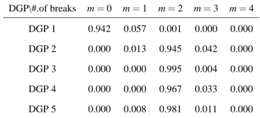
Table 1 summarizes the results of the Monte Carlo simulations. Each element in the Table shows the average posterior probability out of 500 replications for each number of breaks. We compute the posterior probability with Chib’s method described in Section 4. For DGP 1, where there are no breaks, the average posterior probability when m=0 is 94.2%. For DGP 2, 3, 4, and 5, the correct number of breaks, m=2, is detected at about 94.5%, 99.5%, 96.7%, and 98.1% respectively. Thus, the DGP of the VAR models with breaks in volatility (DGP3 and 5) perform better than those of the homoskedastic VAR. Overall most of the iterations choose the correct number of breaks. Table 2 reports that the Monte Carlo mean of estimated break points that are the mode of the posterior when the correct number of breaks m=2 is chosen. The estimates are

3_{Inclan (1993) and Wang and Zivot (2000) use the prior odds as an independent Bernoulli process with probability}

all close to the true values, b= (100,200).

6.2 Monte Carlo Simulation: VECM with Structural Breaks

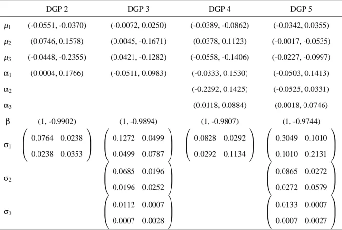
The second experiment is for vector error correction models with multiple structural breaks. We consider the following five data generation processes (DGPs) of a two-variable co-integrated model: DGP 1:∆yt=µ+yt−1βα+σεt DGP 2:∆yt=µt+yt−1βα+σεt DGP 3:∆yt=µt+yt−1βα+σtεt DGP 4:∆yt=µt+yt−1βαt+σεt DGP 5:∆yt=µt+yt−1βαt+σtεt for t=1,2, . . . ,300.

whereεt∼iidN(0,1). DGP 1 represents a no structural break model. DGP 2 is a structural break model in µ only, and DGP 3 allows µ andσto change with breaks. DGP 4 represents a structural break model in µ, α. DGP 5 allows µ, α and σto change with breaks. In both DGP 4 and 5, the cointegrating rank is constant over the whole sample. The parameters given in each DGP 2-5 are shown in Table 3. For the DGP 1, the parameters are set as: µ=µ1 of the DGP 2, and other

parameters are the same as those of the DGP 2. These values are obtained by using Japanese short-and long-term interest rates.

The Gibbs sampling algorithm in Section 3.2 is implemented for the estimation of models for

m=0,1, . . . ,4 break points. For prior parameters, we set the same values forν0,i,ψ0,i, B0, and V0

as used in the previous simulation for the VAR models with breaks to ensure fairly large variance for representing prior ignorance. The cointegration rank and the number of the lags in VECM are assumed known. Also, we assume that correct model specifications are known for each model except the number of breaks. We assign an equal prior probability to each model with i breaks, so that_PrPr₍(_mm₌=₀i)₎=1. After running the Gibbs sampler for 500 iterations, we save the next 2,000 draws

for inference. This procedure is replicated 500 times.

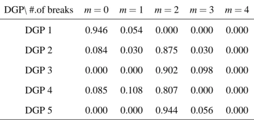
Table 4 summarizes the results of the Monte Carlo simulations for model selection. Each element in the Table shows the average posterior probability out of 500 replications for each num-ber of breaks. Unlike in the previous simulation for the VAR model, the Schwarz BIC method is adopted to calculate the marginal likelihood for the posterior probabilities. The Table shows that in most of the cases the correct number of break points, m=2, is selected with dominantly high posterior probabilities. The heteroscedastic DGPs (DGP 3 and 5) perform better than the ho-moscedastic DGPs (DGP 2 and 4), as in the case of the simulation for VAR models in the previous subsection. DGP 5 shows the best performance with 94.4% of the time for m=2.

Table 5 reports the Monte Carlo mode of the estimated break points. As in VAR models cases, these results show that in most of the cases the estimates are all closed to the true values,

b= (100,200). The results of the homoscedastic DGPs, DGP 2 and DGP 4 show much higher standard deviations in estimating the break points.

7

Application 1: Predictive Power of the Yield Curve

In this section, we illustrate the instability of the predictive power of the yield curve on output growth in the United States as an empirical application of the VAR model with multiple structural breaks shown in Section 2.

7.1 Predictive Power of the Yield Curve on Output Growth

The predictive relationships between the slope of the yield curve and subsequent inflation or real output have been extensively studied. The consumption capital asset pricing model (CCAPM) with habit formation by Campbell and Cochrane (1999) shows that the term structure is related to the future economic activity - positive slopes of the real term structure precede economic expansion and negative slopes precede economic recession. Mishkin (1990a, 1990b), based on the Fisher decomposition, finds that the yield curve can predict inflation. Although Chen (1991), Estrella and Hardouvel (1991) and other studies find a positive correlation between the yield curve slopes and future real economic activities, Estrella et al (2003) suggest verifying the stability of the

relationship because the predictive power may depend on factors that may change over time such as monetary policy reaction function, real productivity, or monetary shocks.

Estrella et al (2003) investigate the instability of the predictive power based on the following model:

ipk,t =β0+β1spt+εt (45) where spt is the spread between the two interest rates of bonds with different maturity; and ipk,t is the future growth rate of industrial production, IPt, at a forecast horizon k and is defined as

ipk,t ≡(1200/k)ln(IPt+k/IPt). We consider the forecast horizon of one year, that is, k=12, as Estrella et al (2003) show that the predictive power of the spread on industrial production is maximum at k=12.

7.2 Estimation Results

Instead of the linear single equation model given in (45), where future growth rate of industrial production is treated as the endogenous variable, we consider VAR models with p=3,4 and 5 lag terms as: Xt =µt+ p

∑

i=1 Xt−iΦi+εt (46) where Xt = (spt,ipk,t) andεt ∼iidN(0,Ωt). That is, we consider a VAR model with structural breaks in the intercept term µ and the volatilityΩ.4The data for this model are, IPt, the US indus-trial production, rl,t, 10-year US treasury rate as a long-term interest rate, and rs,t, the Federal fund rate as a short-term interest rate, based on monthly data obtained from the Saint Louis Federal Reserve Bank. The sample ranges from 1970:01 to 2005:11 with 430 observations. The two vari-ables, spt≡rl,t−rs,tand ip12,t≡100ln(IPt+12/IPt), are plotted in Figure 1. The prior parameters are the same as those used in the Monte Carlo simulation in Section 6.1. The Gibbs sampling is performed with 10,000 draws and the first 1,000 discarded for the VAR models with the number

4_{We also consider other models such thatΦ}

ialso changes with breaks or the homoskedastic models whereΩdoes

not change over time; however, the results prove to be insignificant as the Bayes factors are much lower than those in the model (46).

of structural breaks m=0,1, . . . ,4 and the lags p=3,4 and 5.

Table 6 reports the Gibbs sampling results of model selection for the number of structural breaks, m, and the lag in the VAR, p. A VAR model with m=3 and p=4 results in the highest posterior model probability with 93.15%. Clearly, a VAR model with no break (m=0) is rejected with nearly zero percent of the posterior model probability.

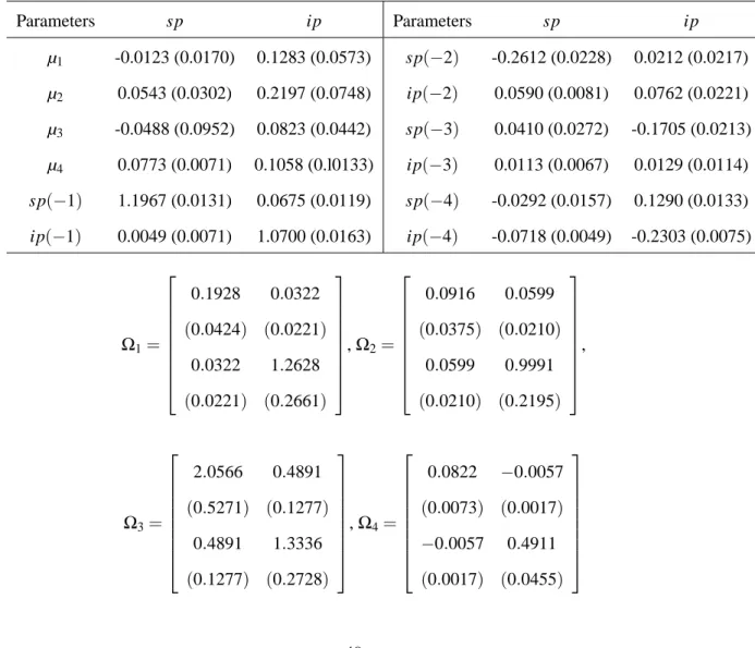
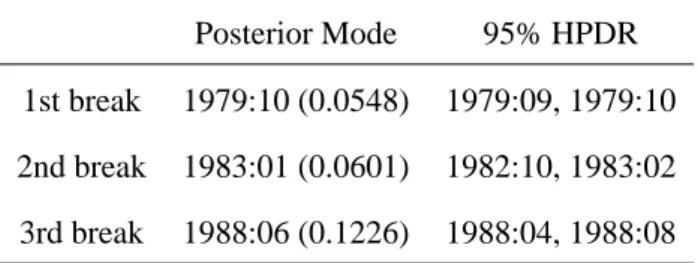
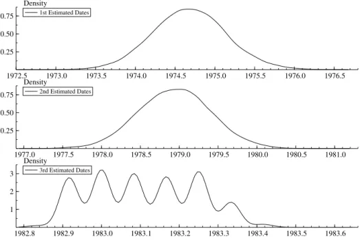
The estimates of the break points and other parameters of the VAR model with m=3 and

p=4 are presented in Table 7. The posterior mass of each break date is plotted in Figure 2. The first break point is detected in the 95% HPDI (Highest Posterior Density Interval) between 1973:09 and 1975:07 with the posterior mode 1974:07. After the first break the variance of the interest rate spread decreased significantly and the productivity growth changed due to the first oil shock. The second break point is detected in the 95% HPDI between 1977:10 and 1979:10 with the posterior mode 1978:11. This second break date is associated with the advent of Fed Chairman Volcker in October 1979, initiating some fundamental changes until October 1982. However, the HPDI of the second date merely covers the assumed break date, October 1979, in the tail. The variance-covariance matrix of the regime between the second and third break dates,Ω3, is much

larger than that of the previous regime, Ω2. The third estimated break date is found between

1982:09 and 1983:03 with the posterior mode 1983:01. This third break date is associated with the completion of the Volcker’s monetary policies of the period with the non-borrowed reserves

operating procedure, while the estimated mode of the third date is not exactly matched with the

assumed date but the HPDI merely covers the assumed date in the tail. After the third break date the variance of both the spread and the industrial productivity growth was much reduced as shown inΩ4.

8

Application 2: US Term Structure of Interest Rates

In this section, we analyze the US term structure of interest rates using the cointegration model with multiple structural breaks presented in Section 3.

8.1 The Expectations Hypothesis

The term structure of interest rates states that the expected future spot rate is equal to the future rate plus a time-invariant term premium. For an overview of the expectations hypothesis theory, see Shiller (1990). The continuously compounded yield to maturity for an f period bond is defined as rf,t =−(1/f)pf,t where pf,t denote the log of the price of a unit-par-value discount bond at date t with f periods to maturity, and the one-period future rate of return, earned from period t+f

to t+f+1, is given by 1+Ff,t=Pf,t/Pf+1,t.Let rf,t denote the yield to maturity f at t. Then the expectations hypothesis implies:

rf,t−r1,t =f−1 f−1

∑

j=1 j

∑

i=1 Et(∆r1,t+i) +Lf (47) where Lf = f−1∑f −1

j=0Λj andΛj is the term premium. If r1,t is integrated of order one, then rf,t must be integrated of order one and yf,t and y1,t are cointegrated with cointegration vector (1, -1), which is analyzed by Campbell and Shiller (1987). This cointegration relationship should be held in any pair of yield to maturity.

However, many studies find that the expectations hypothesis is rejected for US data. Hall et al (1992), and Engsted and Tanggaard (1994) consider this is due to the instability for interest rates between September 1979 and October 1982, known as the period with the non-borrowed reserves

operating procedure. Taking this period into consideration, several studies such as Hansen and

Jo-hansen (1999), Bliss and Smith (1998), and Hansen (2003) show that the expectations hypothesis is held when structural breaks are imposed into the models.

8.2 Estimation Results

We analyze the US term structure of interest rates for detecting structural breaks in a vector error correction model applying the method outlined in Section 3. The data we use are the same as those of the previous application, that is, the Federal fund rate as a short-term interest rate and 10-year treasury bond yield as a long-term interest rate based on monthly data from the Saint Louis Federal Reserve Bank ranges from 1970:01 to 2006:01, with 432 observations. These series are plotted in Figure 3.

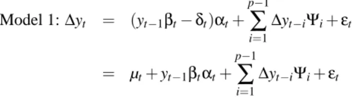
Let yt = (rl,t,rs,t), where rl,t denotes the long-term interest rate at time t and rs,t denotes the short-term interest rate at time t, then the VECM with multiple structural breaks in the coin-tegrating rank, the adjustment term α, the cointegrating vector β, the risk premium δ and the covariance-variance matrixΩcan be expressed from the Granger representation theorem as:

Model 1:∆yt = (yt−1βt−δt)αt+ p−1

∑

i=1 ∆yt−iΨi+εt = µt+yt−1βtαt+ p−1

∑

i=1 ∆yt−iΨi+εt (48)

whereεt ∼N(0,Ω