1
Can the Aggregate Implied Cost of Capital be used to predict excess
returns on the JSE?
Zvikomborero Austen Museka
Supervisor: Dr Odongo Kodongo
Master of Management in Finance & Investment
Faculty of Commerce Law and Management
Wits Business School
University of The Witwatersrand
2 Thesis submitted in fulfilment of the requirements for the degree of
Master of Management in Finance and Investment FACULTY OF COMMERCE LAW AND MANAGEMENT
WITS BUSINESS SCHOOL
UNIVERSITY OF THE WITWATERSRAND
Supervisor: Signature:
DECLARATION
I, Zvikomborero Austen Museka solemnly declare that the research work reported in this thesis is my own, except where otherwise indicated and acknowledged. It is submitted for the degree of Master of Management in Finance and Investment at the University of the Witwatersrand, Johannesburg. This thesis has not, either in whole or in part, been submitted for a degree or diploma to any other university.
---
Zvikomborero Austen Museka
3
Abstract
Return predictability is a principle which has gained increased academic and industry interest over the recent years. A lot of work has been done using different accounting and financial parameters to predict returns on international stock markets. This research sought to find out if we can use the Aggregate Implied Cost of Capital as a proxy for returns on the JSE. The findings show that the ICC is a proxy for returns on the JSE with a reasonably acceptable explanatory power
4
Dedication
This research report is dedicated to
Tinaye Gabriel Museka and Lindiwe Jannet Museka, my dearest two ladies.
5
Acknowledgements
In the past year of lots of hard work, endless sleepless nights and long days, I would like to thank the following people.
Dr. Odongo Kodongo, my supervisor, who was supportive and always present from the inception of the research to the completion and discussion of the findings.
My Wife and little Girl, Lindiwe Jannet and Gabriella Tinaye for your ever present support in all the work.
6
LIST OF ACRONYMS
ICC – Implied Cost of Capital
CAPM – Capital Asset Pricing Model JSE – Johannesburg Stock Exchange
JSE ALSI – Johannesburg Stock Exchange All Share Index OLS – Ordinary Least Squares
APT – Arbitrage Pricing Theory
CAY - Consumption Aggregate Wealth ratio D/E - Debt-to-equity
B/M - Book-to-market value MVE - Market value of equity. S/P - Sales-to-price
7 Table of Contents Abstract ……….………...……… 3 Dedication ………...……… 4 Acknowledgements ………...……… 5 List of Acronyms ………...……… 6 1.0 Chapter Introduction 1.1 Background to the Research Problem ……… 10
1.2 Statement of the problem ……… 11
1.3 Significance of the Study ………. 12
1.4 Objectives of the Research ……… 13
1.5 Research Questions ………..…… 13
Chapter 2: Literature Review 2.1 Theoretical foundations of Factor models for asset pricing ………. 13
2.1.1 CAPM ………...……… 13
2.1.2 The Arbitrage Pricing Theory ……… 14
2.1.3 The Efficient Market Hypothesis and rejection of the CAPM ……. 15
2.1.4 Distribution of Returns and the Random the Walk ……… 16
2.2 The Cost of Capital ………...…… 17
2.2.1 The Implied Cost of Capital ……… 17
2.3 Evidence for Predictability of returns ……… 19
2.3.1Macroeconomic variables ……… 19
2.3.2 Ratios for Predicting Returns on the JSE ……… 20
2.4 The ICC is a good proxy for returns ……… 23
Chapter 3 Data Collection and Research Methodology 3.1 Sampling and Data Collection ……… 25
3.2 Data validity w.r.t OLS Assumptions ……… 25
3.3 Empirical Derivation of the ICC as a proxy for returns……… 27
3.4 Construction of the Aggregate ICC ………. 28
8
Chapter 4 Results
4.1 OLS Assumptions Validity ……… 32
4.2 Excess Returns Calculations ……… 32
4.3 Regression Results ………...…… 34
4.4 Validity of the Results ………... 36
4.5 Standard Forecasting Results .………..………..…… 36
4.6 Discussion of Results ……… 37
Chapter 5 Conclusion 6.0 Appendices ………...……… 40
9
Chapter 1 1.0 Introduction
Market returns information is fundamental in the financial field to investors, traders, institutions, fund managers, retailers and individuals. Required rates of return are important in corporate finance for capital budgeting and for firm valuation purposes. Expected returns information is important for investment management in portfolio allocation, risk control, performance evaluation and style/attribution analysis (Hou, et al., 2012).
It has been reported that trading behaviour of small and large institutions (Dey & Radhakrishna, 2007) change when quarterly earnings are announced. Similarly, studies show that investors learn about future predictability and mispricing from academic publications (Mclean & Pontiff, 2016) and change their positions, if necessary. If predictability is accurate, investors can have maximum returns and profits from the markets. Also on the other hand if predictability is accurate it can be exploited by investors to earn returns greater than the return on the market index (Pesaran & Timmermann, 1995).
Similar studies have been done in the past which show that return predictability does exist. For instance, (Bryan & Seth, 2013) used a single factor extracted from a cross section of book to market ratios to show that returns and cash flow growth for the US stock market are highly predictable. In addition, (Bambang & Setiono, 1998) used financial statements information to predict stock returns in the UK. Also, (Kang, et al., 2010) found that he could predict one year ahead market returns using aggregate accruals in Hong Kong. A part of the sums method (Ferreira & Clara, 2011) was used to predict market returns using a combination of the three components of stock market returns.
In separate studies, (Campbell & Thompson, 2005) argue that the best predictor of future returns is the historical average. Another study by (Balvers, et al., 1990) showed that the returns can be predicted using aggregate output. In other studies, (Pesaran & Timmermann, 1995) and (Rapach, et al., 2005) found that macroeconomic variables have a significant influence in explaining future stock returns. Studies of the Africa’s
10
largest markets of South Africa, Egypt, Nigeria, Kenya, Morocco and Tunisia show that that returns are predictable, both in the mean and variance (Alagidede, 2011).
1.1 Background to the Research Problem
The JSE is one of the world’s 20 largest exchanges by Market Capitalisation ($1,007bn at end-2013 and $1,036bn by August 2016) (JSE, 2016). The JSE is a typical emerging market stock exchange which is regarded as an agent for global risk reduction and potential investment avenues for investors seeking to diversify risk (Alagidede, 2011). This feature is common to other African stock markets too: African stock markets provide benefits of portfolio diversification as they tend to have zero, and sometimes negative, correlation with developed markets (Harvey, 1995)
If the JSE returns can be predicted, then the market can be a good haven for investors seeking to diversify risk and preserve value (Cho, 1986). The availability of returns predictability on the JSE is important to investors so that they can analyse future company performance and structure investment portfolios to obtain the maximum returns (Dreman & Berry, 1995) and (Brown, 1996).
The studies which have been done on predictability on the Johannesburg Stock Exchange (JSE) show conflicting views on whether predictability does exist. In his study, (Mangani, 2007) states that the JSE is not an efficient market hence predictability does exist. Similarly, (Ryan, 2011) using factors representing long-term growth in dividends and earnings and cash flow-to-price ratio to predict returns, found evidence of predictability on the JSE. These results are consistent with the earlier study of (Gupta & Modise, 2011) which showed that traditional valuation ratios have no predictive power on the JSE but the Treasury bill rate, term spread and money supply can predict share returns in the short horizon. Contrarily, (Muzenda, 2014) states that the JSE follows a random walk hence it is not possible to accurately forecast or predict returns of its stocks. However, some other studies have shown that predictability does exist on the JSE.
Recently studies by (Strydom, 2016) explain that the returns on the JSE can be predicted using a different predictor, the consumption aggregate wealth ratio (CAY). (Kruger, 2011), (Gupta & Modise, 2011) and (Strydom, 2016) studies enable us to hold in suspense the notions by (Muzenda, 2014) that return predictability does not exist
11
on the JSE. However, in this paper we would like to find if the implied cost of capital is a predictor for the returns on the JSE in the short and long term horizon. (Cochrane, 2008) states that weak evidence of predicting share returns does not imply that the returns are not predictable but rather that traditional forecasting measures as used by (Kruger, 2011) (Gupta & Modise, 2011) and (I’Ons & Ward, 2012) on the JSE may not be the best predictors.
Hence from the above it is of great value to local and international investors to have a predictor of returns on the JSE. Thus, our study will aim to investigate if the Aggregate Implied Cost of Capital can be used as a good predictor of returns on the JSE.
1.2 Statement of the problem
Can the Aggregate Implied Cost of Capital be a predictor of returns on the JSE? This study will investigate whether the Aggregate Implied Cost of Capital (Aggregate ICC) can be used as a good predictor of returns on the (JSE). The ICC of a firm is the internal rate of return that equates the firm's stock price to the present value of expected future cash flows (Easton & Sommers, 2007). Simplified, the ICC is the discount rate that the market uses to discount the expected cash flows of the firm. The implied cost of Capital is a good indicator as it is derived from discounted expected future cash flows, which take into account future growth opportunities (Pastor, et al., 2008) & (Lee, et al., 2009). This is a better indicator than other methods which predict returns based on realised returns (Blume & Friend, 1973), (Elton, 1999) (Fama & French, 1988) (Fama & French, 1997).
The study investigates the use of the aggregate implied cost of capital as a proxy for market returns on the JSE. Hence this study will add to the literature a predictor for returns on the JSE which can also be adapted for other emerging markets. (Mlambo, et al., 2003) demonstrated that there was significant serial correlation in four African stock markets (Egypt, Kenya, Morocco and Zimbabwe) and hence the findings of this study can be extended to these markets.
1.3 Significance of the Study
The study aims to provide evidence on whether the ICC has predictive power on JSE stocks.
12
The study by (Strydom, 2016) shows that policy makers and investors can use CAY (Lettau & Ludvigson, 2001) & (Sousa, 2012) to predict future business returns and minimise economic downturn and losses on investments. However, these results have
a low explanatory power as measured by R2, the explanatory power for the one-quarter
ahead returns were only 8% based on the CAY. CAY is a significant predictor of
returns but it has to be combined with the term spread to more accurately explain the variation in future returns.
The study by (Gupta & Modise, 2011) using macroeconomic variables to forecast
returns on the JSE also shows low explanatory power, using the R2 coefficient. The
term spread could explain only approximately 4% of the variation in returns in quarter ahead. In the same study Treasury bill yield, could explain only 6% of the one-quarter ahead variation in returns and this value declined as the forecast horizon increased.
The importance of this study is that it aims to close the gap in available findings on the JSE which will give us a predictor which is based on a modern method that takes into account future earnings and growth (Kang, et al., 2010)& (Bambang & Setiono, 1998).
1.4 Objectives of the Research
The objectives of this research are:
To ascertain whether return predictability exists at the JSE stock market
To determine whether the Aggregate Implied Cost of Capital can be used to
predict short term and long term market returns on the JSE
1.5 Research Questions
The following research questions are going to be answered in this study so that we can determine whether the Aggregate Implied Cost of Capital can be used to predict market returns.
Does market predictability on the JSE exist?
What is the correlation between the Aggregate Implied Cost of Capital and
13
Chapter 2: Literature Review
This chapter provides the evidence that we can use the Implied Cost of Capital to predict returns. We set the foundation of returns predictability from asset pricing theories (Fama, 1965) & (Samuelson, 1965) and then highlight the deficiencies of these theories in evaluating the cost of capital. We briefly describe the cost of capital and how we derive the ICC. We then go back to the asset pricing theories and then discuss their assumptions and how they are related to the Efficient Market Hypothesis. We also then discuss the distribution of returns on the JSE in order to have sufficient grounds for predictability. We also discuss the work which has been done in terms of using predictors on the returns. Lastly we discuss the literature which supports the use of the ICC as a predictor and conclude the chapter by discussing the gap which this research will complete and add to the available literature.
2.1 Theoretical foundations of Factor models for asset pricing 2.1.1 Capital Asset Pricing Model CAPM
The classical asset pricing models on the market are the capital asset pricing model (CAPM) of Sharpe (Sharpe, 1964) & (Lintner, 1965) and the arbitrage pricing theory (APT) of (Ross, 1976).
The CAPM is a pricing mechanism for assets on the basis of the relationship between risk and return:
Ra = Rf + βa (Rm – Rf)
Where
Ra = return on the asset
Rf = Risk free rate
βa = beta of the security
Rm = expected market return
The CAPM is a single-factor linear model that relates the expected returns of an asset and the market portfolio, in which the slope, asset beta is a measure of asset non-diversifiable (systematic) risk. If the asset beta and the expected rate of the market
14
portfolio are known or given, the CAPM ‘‘predicts’’ the asset expected rate of return. The CAPM uses a risk-return dominance proposition to ensure fair pricing of assets. Where the equilibrium risk-return relationship is violated, each investor in the market takes a limited position in either the mispriced asset or the market portfolio depending on their risk aversion.
2.1.2 The Arbitrage Pricing Theory
The arbitrage pricing theory (APT) (Ross, 1976) states that the expected return of a financial asset can be modelled as a linear function of various macro-economic factors or theoretical market indices, where sensitivity to changes in each factor is represented by a factor-specific beta coefficient.
ri = ai+ ∑ BNj=i ij Fj+ ui
Where
ri = the realized return on asset i,
ai = a constant for asset i,
Fj = 1… N are orthogonal zero- mean systematic risk factors
ui = the zero-mean idiosyncratic error term
and Bijis asset i's fact or loading (beta) with respect to factor Fj.
The APT states that if asset returns follow a factor structure then there is a linear relationship between expected returns and the factor sensitivities.
E(rj) = rf+ bj1 RP1 + bj2RP2 + ⋯ . . + bjnRPn
Where
RPK is the risk premium of the factor
rf is the risk free rate?
From the APT model the asset price should be equal to the expected end of period price discounted at the rate implied by the model. If the price varies arbitrage should bring it back into line. Under the APT, mispricing requires only a small number of investors to restore equilibrium prices due the possibility of arbitrage enabling investors to take a riskless, costless position to take advantage of the mispricing. This arbitrage mechanism ensures market equilibrium.
15
The CAPM and APT models assume that the equity risk premium varies proportionally with stock market volatility. The models require that periods of high excess stock returns coincide with periods of high stock market volatility, implying a constant price of risk. It has been well-established in the literature that there are certain firm characteristics (often referred to as styles or style anomalies) that appear to be proxies for risks not captured by the traditional CAPM model. The most prominent of these include firm size (Fama & French, 1992) dividend yield (Fama & French, 1988) price-earnings ratios (Basu, 1977) and book-to-market ratio (Fama & French, 1992). Many of these factors have been demonstrated as being significant across markets indicating that there is evidence of global commonality and consistency in these drivers of risk (see Haugen and Baker, 1996).
2.1.3 The Efficient Market Hypothesis and rejection of the CAPM
The efficient-market hypothesis (EMH) states that asset prices fully reflect all available information. A direct implication is that it is impossible to "beat the market" consistently on a risk-adjusted basis since market prices should only react to new information or changes in discount rates (the latter may be predictable or unpredictable (Fama, 1965). (Grossman & Stiglitz, 1980) suggests that market efficiency is impossibility. Market efficiency is pre-supposed upon the action of market participants in integrating new information into existing stock prices. Such action is not, however, rewarded by the market as efficiently-priced assets provide no possibility of abnormal returns above the fair value of the asset. There is therefore no incentive for market participants to facilitate the gathering and processing of information and the price adjustment mechanism will fail as a consequence.
In an efficient market, both the CAPM and APT models suggest that assets should be
fairly priced in equilibrium. However, in deriving the CAPM (Sharpe, 1964) and
(Lintner, 1965 ) assumed that there was a riskless asset in the investment opportunity set, and the first significant extension of their work was by (Black, 1973) who showed that the assumption of a riskless asset could be dispensed with. The static equilibrium in which risk is a constant does not hold because there are a number of factors that lead to a reduction in a firm’s cost of capital apart from risk. These include variation in
16
the firm’s cash flow, number of shareholders in the market, increased risk tolerance in the market and expectation for increased cash flow (Lenz & Verrecchia, 2005).
The Arbitrage Pricing theory (APT) and CAPM are linear and static models based on the assumption that the prices follow a normal strong random walk (Campbel, et al., 1997). If the returns follow a random walk they are normally, independently and identically distributed, or iid normal. This finding is akin to the Efficient Market Hypothesis, EMH (Fama, 1965) which states that in an efficient market, market prices fully reflect all available information hence returns are not predictable. It is not possible to earn excess returns on the market by using all available information because the prices of securities in the market should be equal to their intrinsic value and reflect a present value of a rational forecast of the expected future dividend payments. 2.1.4 Distribution of Returns and the Random the Walk
Studies by (Hsieh, 1989.), provide evidence that stock returns are not independently and identically distributed as assumed by EMH. Empirical evidence on the time series properties of security prices documented for most markets is strikingly against the normal strong random walk property (Kasch-Haroutounian & Price, 2001). (Page, 1993) provides compelling evidence that JSE security returns are not normally
distributed. The results of both parametric and non-parametric tests show that the
South African stock market is weak form efficient (Simons & Laryea, 2005). Further
studies by (Makakabule, et al., 2010) show that the JSE violates the weak and semi
strong form test of the efficient market using macroeconomic variables.
In addition if the stocks are not iid normal, then the stock prices exhibit permanent and transitory components and there is volatility on the stock market (Lettau & Ludvigson, 2001 ). (Smith, et al., 2002) found that the South African stock market followed an iid random walk. Hence there exists a possibility of characterising a nonlinear relationship between stock returns and economic fundamentals.
According to (Summers & Schleifer, 1990), nonlinearities in stock returns can arise due to noise trading, long memory in stock returns due to time variation in expected
17
2.2 The Cost of Capital
The cost of capital is defined as the return that equates the price of a firm to its cash flow (Fama, 1976.). 𝑃𝑗 = 𝐸 ⌊𝑐𝑗⌋ 1 + 𝑅𝑗 Or 1 + 𝑅𝑗 = 𝐸 ⌈𝐶𝑗 ⌉ 𝑃𝑗 Where
cj is uncertain cash flows of firm j
Pj is the market equilibrium price of firm j, Rj is the cost of capital.
This characterization of the cost of capital is widespread in accounting and finance and it is used in discounted cash flow models valuing firms or in capital budgeting. Similarly, it is employed in estimating the implied cost of capital from analyst forecasts (Botosan & Plumlee, 2005); (Gebhardt, 2001)
2.2.1 The Implied Cost of Capital
The implied cost of capital (ICC) for a given asset can be defined as the discount rate (or internal rate of return) that equates the asset’s market value to the present value of its expected future cash flows.
In recent years, a substantial literature on ICCs has developed in accounting and finance. In finance, the ICC methodology has been used to test the inter temporal CAPM (Pastor, et al., 2008), international asset pricing models (Lee, et al., 1999) and default risk (Chava & Purnanadam, 2009) In each case, the ICC approach has provided new evidence on the risk return relation that is more intuitive and more consistent with theoretical predictions than those obtained using ex post realized returns (Fama & French, 1997 ) and (Pastor & Stambaugh, 1999). The collective evidence from these studies indicates that the ICC approach offers significant promise in dealing with a number of long-standing empirical asset pricing conundrums. The standard asset pricing models fail to provide precise estimates of the firm-level cost of equity capital (Lee, 2010).
18
This section will provide evidence on predictability of returns on and then further highlight evidence of economic variables used to predict JSE returns.
The debate that stock market returns follow a random walk and are not predictable because markets are efficient (Fama, 1965) has been discarded by replete literature that shows that stock prices are non-normal, non-linear and partially predictable (Bollerslev T, 1994) & (Blake, 2000) & (Malkiel, 2003).
Further analysis of the JSE returns by (Auret & Sinclaire, (2006)) show that returns is mean reverting and this implies that future stock prices can be predicted from historical prices. If the returns are mean reverting then the market is not efficient and this is similar to the findings by Page and Way (Fraser & Page, 2000) based on the foundational studies by (Bandt & Thaler, 1985).
The evidence for predictability of stock returns is based on two empirical principles, permanent and transitory components of stock prices and volatility of the stock market. In the literature by (Fama & French, 1988) found that negative autocorrelations in stock prices signify mean reversion in stock returns thus implying that stock returns have a transitory component and are predictable. In the literature on stock market volatility,
(LeRoy & Porter, 1981) & (Shiller, 1981) show that stock returns exhibit “excess
volatility,” which is indirect evidence that the returns can be forecasted. If excess stock market returns are predictable, the conditional mean of excess returns moves over time.
In studies to find the relationship between stock returns and macroeconomic variables, (Jefferis & Okeahalam, 2000) authors found that stock returns in South Africa, Botswana and Zimbabwe were driven by real exchange rate, long-term interest rates and GDP. In other separate studies (Rensburg, 2000) examined the impact of macroeconomic variables on the JSE stock returns using the Arbitrage Pricing Theory (APT) and found that stock returns on the Johannesburg Stock Exchange (JSE) are driven mainly by resource and industrial sectors in South Africa. The macro economic variables can be seen as indicators of the fundamental value of the stock, relative to the current price. The idea of using these as predictor variables is that variation in the macroeconomic variables should reflect variation in the market’s rational expectation
19
of the future value of stock returns and dividend growth or earnings growth respectively (Rasmussen, 2006).
Using a wide range of tests for normality, (Page, 1993) confirmed the presence of non-normalities in equity returns on the JSE. Using nonparametric runs tests, he also found evidence suggesting that the security returns were non-stationary processes.
The work by Page gives evidence that returns on the JSE can be predicted. According to (Mangani, 2007) the returns on the JSE were highly leptokurtic, displayed excess skewness (which could be positive or negative), and were far from being iid. In his study, Mangani rejected the hypothesis that log returns were normally and linearly distributed and the underlying stock prices followed a log normal strong random walk process.
Hence by selecting the appropriate economic indicators we can predict returns of stocks. Hence we can violate the notion that the JSE is an efficient market in which we cannot predict the returns (Muzenda, 2014) and in this study we will investigate whether we can use the ICC to predict returns on the JSE.
2.3.1Macroeconomic variables
(Fama & French, 1989) show that the yield spread between low- and high-grade corporate bonds, the default premium, can be used as a predictor variable for long horizon stock returns. The intuition is that the default premium, def, is an indicator of general business conditions and hence should be able to capture long-term business cycle variation in stock returns. (Campbell, 1991) & (Hodrick, 1992) suggest using
another macro variable, the relative bill rate, rtb, to forecast future stock returns.
The study by (Schwert, 1990) gives evidence of a strong relationship between stock returns and macroeconomic variables when examining whether predictability is attributed to time variation in expected returns. Evidence from (Chang, 2009) and (McQueen & Roley, 1993) shows that predictability of stock returns shows asymmetric behaviour and the relationship is stronger in bad times (recession) than in good times (economic boom).
20
Macroeconomic variables such as inflation rates, term and default spread on bonds, aggregate output, money supply, exchange rates and unemployment rates are found to have significant influence in explaining stock returns (Rapach, et al., 2005). In addition, (Pesaran & Timmermann, 1995) provide evidence of predictable components in stock returns using macroeconomic variables such as interest rates, dividend yields, economic growth (industrial production) and inflation. The authors find the existence of a relationship between stock returns and macroeconomic variables, even after accounting for transaction costs. They ascribe the existence of predictability in stock returns to incomplete learning and the presence of time-varying premium.
On the JSE, selected South African macroeconomic variables (MacFarlane & West, 2013) explain an insignificant portion of future returns on the FTSE/JSE All Share Index returns. The hypothesis for each of the macroeconomic variables to predict market returns are briefly explained. An increase in GDP (Gan, et al., 2006) output may increase future expected cash flows and subsequent profitability; hence GDP will have a causal effect on the ALSI. CPI (Humpe & MacMillian, 2009) is a proxy for inflation. When Inflation rises a firm ‘s production costs and therefore decreases its future cash flow which lowers revenue as well as profits. Hence CPI will be negatively correlated with stock prices. An increase in interest rates raises the required rate of return (Alam & Uddin, 2009), which in turn inversely affects the value of the asset. The appreciation of the rand dollar exchange rate is hypothesised as being inversely related to the stock price index. Hence money supply (Humpe & MacMillian, 2009)
may have either a positive or negative effect on stock prices returns.
Other studies have been able to show that the returns on the JSE can be successfully predicted. The paper by (Gupta & Modise, 2011) shows that the Treasury bills rate, term spread and money supply are able to predict share returns at a relatively short horizon. The study concluded that valuation ratios have no forecasting power on future returns. The study done by (Kruger, 2011) shows that there is evidence of linear and nonlinear predictability in index returns on the JSE but with weak evidence.
2.3.2 Ratios for Predicting Returns on the JSE
Four main approaches are used by analysts to identify investment opportunities, namely discount dividends, asset evaluation, cash flow analysis and relative valuation
21
(Clemente, 1990). A wide range of ratios based on financial and macroeconomic variables have been introduced in the predictability literature in recent years. These variables can be seen as indicators of the fundamental value of the stock, relative to the current price. The idea of using these as predictor variables is that variation in the ratios should reflect variation in the market’s rational expectation of the future value of stock returns and dividend growth or earnings growth respectively (Rasmussen, 2006).
In his study on the JSE, (Farinha, 2004) used a number of explanatory variables to determine which variable has the best explanatory power for market returns. The following variables were used in the study Debt-to-equity (D/E), Book-to-market value (B/M), Market value of equity (MVE) and Sales-to-price (S/P) ratio.
All the variables were regressed with the returns data and the findings show that the MVE when combined with the B/M ratio had the highest explanatory power for returns compared to other variables. Hence the BTM still retained a lower explanatory power to predict market returns on the JSE.
Prior to Farinha’s work, (Rensburg & Robertson, 2003) employed both a univariate and paired factor multiple-regression methodology to determine the ability of 24 firm specific attributes to explain average monthly returns on the JSE over the period July 1990 to June 2000. They found that price-to-net asset value (NAV), dividend yield, price-to-earnings ratio, cash flow-to-price and size are all significant explanatory variables of returns.
Book to Market Ratio Book-to-market ratio (BTM) compares the book value of a firm to its market value (Fama, 1990). The studies by (Fama & French, 1992) found a strong positive BTM effect, on returns suggesting that firms with higher BTM ratios have higher expected average returns.
(Auret & Sinclaire, (2006)) Show that the book-to market ratio is a good predictor of returns on the JSE (in the cross-section at least), but after they include all of the ratios in a cross-sectional regression the cash flow yield is the only significant variable.
22
(Basiewicz & Auret,2009) extended on the work by (Auret & Sinclaire, (2006), examining a broader selection of firm characteristics for evidence of return predictability. They corrected for thin trading and transaction costs and employed independent rather than sequential sorts and both value- and market-weighted compositions in their portfolio tests. They found that both size and book-to-market were significant explanatory variables in their regressions, contradicting the finding of (Auret & Sinclaire, (2006)) that book-to-market subsumes the size effect, although book-to-market is the most significant of the factors examined. The authors suggested that this is due to the strength of the size factor over the period 2003 to 2005 which was not included in the previous study.
Dividend-to-price-ratio (D/P)
Divided to price ratio indicates how much a company pays out in dividends each year relative to its share price. (Shiller, 1988). The findings by (Litzenberger & Ramaswamy, 1979) show that dividend yield exhibits positive correlation with average returns. The study by (Andrew Ang, 2006) also explains that although predictability exists it is mainly for the short-horizon and not the long-horizon. Finally, dividend and earnings yields have good predictive power for future cash flow growth rates, but not future excess returns. Hence, a potentially important source of variation in price-earnings and price-dividend ratios is the predictable component in cash flows (Andrew Ang, 2006).
Price-to-earnings ratio (P/E)
P/E is the ratio of a company's share price to its per-share earnings (Morse, August 1978). Other scholars (Ball, 1978) argue that the E/P ratio is a blanket proxy for unnamed risk factors in expected returns. In the U.S, early tests found that the dividend-to-price and earnings-to-price ratios were able to forecast future returns (Fama & French, 1988) & (Hodrick, 1992). However, (Lamont, 1998) demonstrated that the dividend-to-price ratio had greater predictive power than earnings-to-price. More recently, (Ang & Bekaert, 2007) and (Lettau & Ludvigson, 2001) confirmed the ability of the dividend-to-price ratio to predict excess returns over short and long horizons, but only when combined with a measure of the short-term interest rate.
23
Composite Ratios
Some other ratios have been introduced on the market which appears to capture movements in stock prices, which traditional ratios are not able to. (Rangvid, 2006) shows the output ratio outperforms the traditional dividend yield and price-earnings ratio when predicting long-horizon returns. The financial ratios are usually combined with other measures such as short term interest rate and term spread (Kein, December 1986) in order to adequately forecast future returns (Rasmussen, 2006). (Menzly, et al., 2004) suggest that expected excess stock returns are a linear function of the dividend yield and price-consumption ratio, pc. (Julliard, 2004) Develops further on the consumption aggregate wealth ratio (CAY) variable. He uses the assumption that labour income is not approximately a random walk and takes into account expectations of future labour income growth when using cay to forecast stock returns. (Benzoni, et al., 2006) proposes a two-variable relation between dividends and labour income, unlike the trivariate relation underlying CAY in order to forecast returns. On the JSE, (Strydom, 2016) followed the work by (Sousa, 2012) to use a composite predictor, the consumption aggregate wealth ratio (CAY) (Lettau & Ludvigson, 2001) to forecast share returns. His results show that the CAY is a significant predictor of returns but it has to be combined with the term spread to more accurately explain the variation in future returns.
2.4 The ICC is a good proxy for returns The ICC has been widely used in forecasting returns in Accounting and Finance
research as it is an appealing proxy for future returns (Li, et al., 2013; Hou, et al.,
2012; Guay, 2011; Easton, 2005; Gebhardt, 2001). (Gebhardt, 2001) & (Gode P,
2003)show that there is a positive relationship between average future returns and
portfolio rankings based on the Implied Cost of Capital.The key reason for the ICC's
superior performance is that the ICC is estimated from a theoretically justifiable discounted cash flow valuation model that takes into account future growth
opportunities that are ignored by traditional valuation ratios (Kang, et al., 2010) and (Bambang & Setiono, 1998). Literature shows that there is a positive correlation between the ICC and market returns (Lee, 2010) and the various methods of
calculating the ICC cannot discredit the relationship. There is evidence from (Hou, et al., 2012) that the future market returns can be better predicted by using a
model-24
based ICC which uses cross sectional data compared to analysts’ forecasts. The cross sectional based ICC has a time-series coverage which uses the large cross-section of individual firms to compute earnings forecasts and therefore generates statistical power which can explain a large fraction of the variation in expected profitability across firms (Hou & Robinson, 2006).
In addition, (Yan Li, 2013) successfully demonstrated that the aggregate ICC strongly predicts future excess market returns at horizons ranging from one month to four years. The work by (Pastor, et al., 2008) demonstrates that if the conditional expected return follows an AR (1) model, the resultant ICC is linearly related with the conditional expected return. Recently (Azevedo, 2016) provided evidence that the ICC is able to predict returns over time at the aggregate level and the firm level using the Claus and Thomas (Claus J, 2001) and (Gebhardt, 2001) approach respectively.
From the above we can conclude that there is sufficient literature that the ICC is able to predict equity returns but the reliability of the prediction is based on the method of the construction of the ICC.
According to (Hou, et al., 2012; Lee, 2010) the choice of method for constructing the ICC has an impact on the reliability of the returns predictability. According to (Hou, et al., 2012) a cross sectional based ICC is more reliable than an analyst-based ICC. The analyst’s based ICC relies on the quality of analysts’ earnings forecasts which in most cases exhibit biases of over optimism due to their conflicts of interest (Gebhardt, 2001). Studies done by (Gebhardt, 2001), (Easton, 2005) and (Guay, 2011) exhibit mixed results for the relation between the analyst-based ICC and future realized returns. In addition, Easton and Monahan (2005) show that the analyst-based ICC has little predictive power for future realized returns after controlling for cash flow news and discount rate news.
In order to fill the gap which exists in industry, this study will focus on investigating whether the ICC is a predictor of returns with high explanatory power in the short and long horizon. The existing parameters either provide weak evidence of predictability such as macro variables or have to be combined with other parameters such as consumption aggregate wealth ratio to show predictability.
25
Chapter 3 Data Collection and Research Methodology
3.1 Sampling and Data Collection
The primary data used in this analysis was yearly close prices for each of the individual stocks and portfolios. The yearly observations are preferable because previous work done on the JSE on returns uses yearly data and this gives a large data sample size for comparison with previous findings (Mangani, 2007); (Muzenda, 2014) & (Ryan, 2011).
The study period will be from 02 January 2001 to 31 December 2016 for the individual stocks. The data sample period is chosen for a fifteen-year period in order to give us an opportunity to test for the ICC predictability in the short and long horizons. Studies by (Lettau & Ludvigson, 2001)show that the chosen predictor CAY had the strongest forecasting ability short and mid-range whereas other studies show that prize normalized variables such as the price-consumption ratio of (Menzly, et al., 2004) and the price-output variable of (Rangvid, 2006) outperform the other variables in the long horizons. Hence by choosing a sample of fifteen years we have an opportunity to determine whether the ICC is a predictor of returns on the JSE in the short term and long term. The period 2001 to 2006 will act as the in sample period. The short term horizon will be extended to 2011 because of the market crisis from August 2007 to December 2009 (Kruger, 2011).
The close price data on the individual stocks was obtained from Bloomberg. The final sample of the study will comprise the top 100 listed shares from the industrial, resource and financial sectors because they account for approximately 90% of the entire JSE the total market capitalisation (Ryan, 2011).
Yearly returns will be obtained for the overall JSE from INET Bridge data source.
3.2 Data validity w.r.t OLS Assumptions
The data validity w.r.t OLS is important because standard testing procedures such as regression in a time series model, require that the respective variables are
stationary since most econometric theory is built upon the assumption of stationarity (Verbeek, 2009).In this study we will test the yearly stock prices for stationarity.
26
In order to add to the literature and validate whether returns for our sample data can be predicted, we will test their distribution for autocorrelation. In addition, we will test the characteristics of the returns obtained for the stocks for normality and linearity in order to evaluate whether the returns follow a random walk or not.
3.2.1 Testing for Stationarity
To apply standard testing procedures such as regression in a time series model, it is normally required that the respective variables are stationary since most econometric theory is built upon the assumption of stationarity (Verbeek, 2009). Stationarity is defined by (Challis & Kitney, 1991)as a quality of process in which the statistical parameters such as the mean, standard deviation autocorrelation and other parameters do not change with time and depends on the lag alone at which the function was calculated. This is critical as without the normal distribution, the subsequent time series analysis will give incorrect results. When time series data does not follow the normal distribution due to fluctuations, that data is non-stationary. The non-stationarity of a series can influence its behaviour and properties substantially. Verbeek (2008) stipulates that regressing a non-stationary variable upon another nonstationary variable may lead to spurious regression. Thus any correlation between two such variables is misleading as it does not entail causation.
In order to test for stationarity in each of the variables in our sample, we used the standard Dickey-Fuller (DF) (Fuller, 1976)and augmented Dickey-Fuller (ADF) tests (Said & Dickey, 1984):).
3.2.2 Testing for Random Walk.
In general, data are said to satisfy the normality property if their probability density function is consistent with that of a normally distributed random variate. The Jarque– Bera test will be used to test whether the sample data have the skewness and kurtosis matching a normal distribution. The null hypothesis is a joint hypothesis of the skewness being zero and the excess kurtosis being zero. Samples from a normal distribution have an expected skewness of zero and an expected excess kurtosis of zero (which is the same as a kurtosis of 3) (Jarque & Bera, 1981).
27
Further, a series is said to satisfy the linearity property if it is an independently and identically distributed (iid) process. When both the normality and linearity properties are satisfied in the return series, the underlying price series is said to follow a normal strong random walk process. Else, when the return series is non-normal but iid, price follows a strong random walk process. Our interest in these properties derives directly from static asset pricing theory, which assumes joint multivariate normality and linearity as characterising the distributions of returns.
3.2.3 Testing for Autocorrelation The Breusch Godfrey test will be used to test for the presence of serial correlation under the null hypothesis that there is no serial correlation of any order up to p (Breusch, 1978).
3.2.4 Co-integration Lastly after obtaining our results we will test for co-integration between the excess
returns and the ICC. Co-integration analysis (Johansen, 1991) is used to determine the long term relationship between the Implied Cost of Capital and the stock market. Verbeek (2008) notes that co-integration is a statistical property of a time series where variables are co-integrated if they each share a common trend or they share a certain type of similarity in terms of their long-term fluctuations; however, they may not automatically move together and may be otherwise unrelated.
3.3 Empirical Derivation of the ICC as a proxy for returns
The research will go on to explain how we derive the ICC to be analysed as a good proxy for returns.
There are five methods of estimating the ICC which are classified into three main categories: ( Claus and Thomas and Gebhardt et al.) based on the residual income valuation model (Claus J, 2001) (Gebhardt, 2001); (Ohlson and Juettner-Nauroth and Modified Price-Earnings Growth) are abnormal earnings growth-based models (Ohlson, 2005); Gordon is based on the Gordon growth model (Gordon, 1997). The difference of the ICC estimates is due to different ways to forecast earnings, the explicit forecast horizon, and the assumptions regarding short-term and long-term growth rates.
28
According to (Hou, et al., 2012; Lee, 2010) the choice of the construction of the ICC has an impact on the reliability of the returns predictability. According to (Hou, et al., 2012), a cross sectional based ICC is more reliable than an analyst-based ICC. This is because analyst’s based ICC relies on the quality of analysts’ earnings forecasts which in most cases exhibit biases of over optimism due to their conflicts of interest (Gebhardt, 2001). In separate findings, (Guay, 2011) obtained mixed results for the relation between the analyst-based ICC and future realized returns. In addition, (Easton, 2005) shows that the analyst-based ICC has little predictive power for future realized returns after controlling for cash flow news and discount rate news. The cross sectional based ICC has a time-series coverage which uses the large cross-section of individual firms to compute earnings forecasts and therefore generates statistical power which can explain a large fraction of the variation in expected profitability across firms (Hou & Robinson, 2006).
3.4 Construction of the Aggregate ICC The aggregate ICC is the weighted average of the ICC of firms under consideration,
and the weight is based on the firms’ market capitalisation.
In order to calculate the firm level ICC, each firm needs a one, two or three years
ahead forecast. In order to calculate the firm level ICC, we need to solve for re in the
infinite horizon dividend discount model equation below.
𝑃𝑡 = ∑∞ ((1+𝑟𝑒)𝐸𝑡(𝐷𝑡+𝑘)𝑘)
𝑘=1 (1)
Where Pt = stock price
Et = market expectations based on information available in year t Dt = dividend at time t Re = The cost of capital
In our study we are going to construct an estimate for the earnings forecast for a 15-year period.
3.5 Methodology Steps
Step 1: Obtaining the ICC
𝑃𝑡 = ∑ 𝐹𝐸𝑡+𝑘(1+ 𝑟 𝑥 (1− 𝑏𝑡+𝑘)
𝑒)𝑘
𝑇
𝐾=1 + 𝑟𝐹𝐸𝑡+𝑇+1
29
We will log-linearise the equation above and obtain the discount rate that the market uses to discount the expected cash flows of the firm as calculated above. The value used to discount the cash flows is the ICC.
The ICC can be obtained from the above equation by calculus, making re the subject of the formulae and hence solving for re by using the iteration below:
Calculation of Implied Cost of Capital
𝑟𝑒1= (1 − 𝑌 ∗)11− 1 𝑟𝑒2= (1 − 𝑌 ∗)12− 1 𝑟𝑒3= (1 − 𝑌 ∗) 1 3− 1 𝑟𝑒𝑛= (1 − 𝑌 ∗)𝑛1− 1 (3)
Where n is the year and
Y* is the known term from previous estimated cash flows and calculated ren-1 AND the ICC of each firm can also be obtained by log linearizing the above equation and obtaining the values of re which solve for the equation below for each of the firms.
𝑟𝑒,𝑡= 𝑘 + (1 − 𝜌)(𝑑𝑡− 𝑝𝑡) + (1 − 𝜌)𝐸𝑡(∑∞𝑗=0𝜌𝑗 ∆𝑑𝑡+1+𝑗) (4)
Where 𝑟𝑒,𝑡 = the log stock return at time t
𝑑𝑡 = the log dividends at time t
𝜌 = 1/(1 + exp(𝑑 − 𝑝))
𝑘 = - log (𝜌) -(1 − 𝜌)𝑙𝑜𝑔 (1𝜌− 1)
𝑑𝑡− 𝑝𝑡= the average log dividend-to-price ratio
Both methods are going to be employed in this study in order to have a spectrum of what will be the best methodology to use in order to interpret the excess returns. Forecasted Earnings will be calculated using the growth rates which will be used to
30
each firm needs to have a one-year-ahead, a two-year-ahead and three-year-ahead mean earnings forecast. If a three-year ahead forecast is not available, we will use the consensus long-term growth rate to estimate it. Moreover, if neither the three-year ahead earning forecast nor the long-term growth rate is available, we will compute the growth between one-year and two-year ahead earnings forecast as an implicit growth.
The 12 month ahead forecasted earnings for the next period, t+1 is obtained by
calculating a monthly weighted average of the Earnings per Share in the period over which the Earnings per share are obtained.
The 24 months ahead forecasted earnings are then obtained by using the intrinsic growth rate exhibited by the variance in the Earnings Per Share forecasts (net income
/ # of shares outstanding) for Year t+2 and t+1.
𝐹𝐸2 = 𝐹𝐸1 𝑥(1 + 𝑔2) (5)
Where 𝑔2 = 𝐹𝑌2 / 𝐹𝑌1−1
The 36 month forecast and the periods beyond is obtained by assuming that from year
t+2, there is steady state growth and g2 becomes a constant. We also assume that the
growth rate g2 is equal to the long run average annual GDP.
This means earnings and growth rates for the periods t + 3 to t+T +1 are computed as per the below (k -3; …. T +1)
𝑔𝑡+𝑘 = 𝑔𝑡+𝑘−1 𝑥 exp[log(𝑔 𝑔⁄ )/𝑇]2 (6)
𝐹𝐸𝑡+𝑘 = 𝐹𝐸𝑡+𝑘−1 x (1 + 𝑔𝑡+𝑘) (7)
Plowback Rates
The plowback period in the 12 months’ period ahead, b1 is obtained as one minus the most recent dividend pay-out ratio. The dividend pay-out ratio is dividends/ earnings. In order to calculate the intermediate plow back rates from t+2 to t+T, we assume that the 12 month forecasted plowback becomes constant in the terminal period t+T+1. Hence, the intermediate plow back rates from t +2 to t + T (k= 2…T) are computed as bt+k = b t+k-1- (b1 –b)/T.
31
The constant b is obtained from the sustainable growth rate model, g=(1-b) ROE. The ROE is obtained from Return on Equity = Net Income/Shareholder's Equity
The steady-state plow back rate b is then obtained as g=re.
Net income is for the full fiscal year (before dividends paid to common stock holders but after dividends to preferred stock)
Shareholders equity does not include preferred shares. Step 2: Obtaining the Aggregate ICC
After obtaining the firm level ICC, we then obtain the Aggregate ICC. The weight is based on the market capitalisation of the firm in the month under consideration. Step 3: Obtaining the Excess Returns
We estimate the aggregate ICC by value-weighting the ICCs of the top 100 firms in the JSE each month.
We then subtract the three-month T-bill yield from the aggregate ICC to compute the excess ICC (the implied risk premium) and use it to forecast future excess market returns.
Step 4: Forecasting and Forecasting Horizon
Forecast horizon – calculated in months, being the difference between announcement date and year-end date year end forecast months.
FH = [Date year end – Date forecast] years (8)
We will use the Standard forecasting regression methodology to examine the predictive power of the ICC.
The correlation factor for the in sample period and out of sample period will give us an idea of the predictive power of the ICC.
Step 5: ICC comparison with other predictors
We will compare the outcome and performance of the ICC with other forecasting variables which have been used on the JSE, namely term spread, treasury bill (Gupta & Modise, 2011) and consumption aggregate wealth (Strydom, 2016).
32
Chapter 4: Results The data was first tested for the standard Ordinary Least Squares Assumptions.
After the OLS assumptions were met, the research then went on to carry out regression analysis on the data.
4.1 OLS Assumptions Validity
Stationarity: The Augmented Dickey-Fuller (ADF) tests in Appendix 1show that the data for the JSE returns is stationary at 1% significance level.
Normality: The Results in Appendix 2 show that the excess returns follow a normal distribution because the p value for the JB test is 32% which is greater than 5% significant level (Jarque & Bera, 1981).
Since the data shows Stationarity and Normality which satisfies the Ordinary Least Squares assumptions reference we went ahead to use the Standard Regression methods to determine the relationship between the Aggregate Implied Cost of Capital and the Excess Returns on the JSE.
4.2 Excess Returns The analysis uses two sets of T Bills to analyse the excess returns to give an idea of
the correlation of short term excess returns and long term excess returns. The two T – Bills used are the 3-month T Bill and the 10 Year T Bill respectively.
33
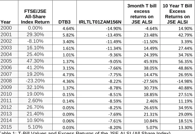
Table 1: T Bill Values and Excess Returns
The table below gives the annual values calculated for the annual excess returns.
Year
FTSE/JSE All-Share
Index Return DTB3 IRLTLT01ZAM156N
3month T bill excess returns on JSE ALSI 10 Year T Bill Excess Returns on JSE ALSI 2000 0.00% 4.64% -14.90% -4.64% 14.90% 2001 29.30% 5.82% -13.49% 23.48% 42.79% 2002 -8.10% 3.40% -11.49% -11.50% 3.39% 2003 16.10% 1.61% -11.34% 14.49% 27.44% 2004 25.40% 1.01% -9.36% 24.39% 34.76% 2005 47.30% 1.37% -9.05% 45.93% 56.35% 2006 41.20% 3.15% -7.66% 38.05% 48.86% 2007 19.20% 4.73% -7.75% 14.47% 26.95% 2008 -23.20% 4.36% -8.22% -27.56% -14.98% 2009 32.10% 1.37% -8.78% 30.73% 40.88% 2010 19.00% 0.15% -8.51% 18.85% 27.51% 2011 2.60% 0.14% -8.59% 2.46% 11.19% 2012 26.70% 0.05% -8.25% 26.65% 34.95% 2013 21.40% 0.09% -7.69% 21.31% 29.09% 2014 10.90% 0.06% -7.61% 10.84% 18.51% 2015 5.10% 0.03% -8.20% 5.07% 13.30%
Table 1: T-Bill Values and Excess Returns of the JSE ALSI (All Share Index)
Where DTB3 is the 3 Month Treasury Bill
IRLTLT01ZAM156N is the 10 Year Treasury Bill
FTSE/JSE All Share index return is the % return from the all share index The excess Returns for the 3 Month and 10 Year Treasury Bill are obtained by subtracting the T-bill in each particular year period from the JSE all share index return. A case example, the excess returns in 2012 are calculated as per the below:
3 Month T Bill excess returns = 26.70 % - 0.05% = 26.65%. 10 Year T-bill excess returns = -8.25% - 26.65% = 34.95%
34
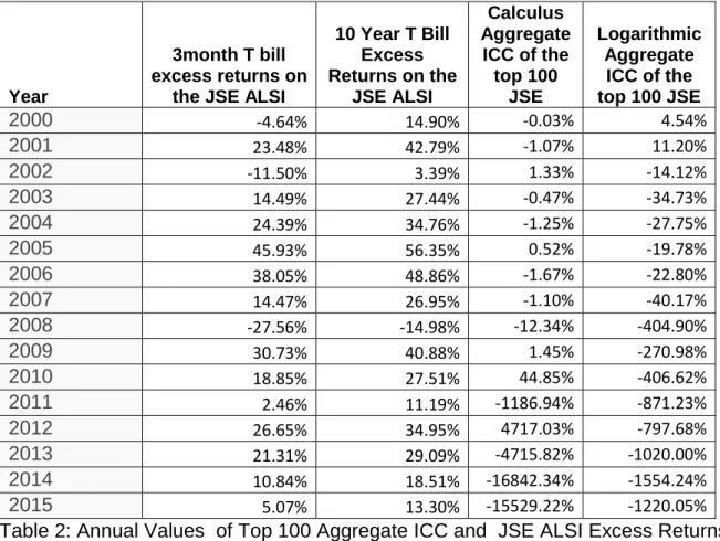
Table 2: Calculus ICC and Logarithmic ICC The table below gives the annual values of the ICC based on the two methods
described in the methodology. Calculus ICC is obtained by solving for equation (3) and Logarithmic ICC is obtained by solving for equation (4).
Year
3month T bill excess returns on
the JSE ALSI
10 Year T Bill Excess Returns on the JSE ALSI Calculus Aggregate ICC of the top 100 JSE Logarithmic Aggregate ICC of the top 100 JSE 2000 -4.64% 14.90% -0.03% 4.54% 2001 23.48% 42.79% -1.07% 11.20% 2002 -11.50% 3.39% 1.33% -14.12% 2003 14.49% 27.44% -0.47% -34.73% 2004 24.39% 34.76% -1.25% -27.75% 2005 45.93% 56.35% 0.52% -19.78% 2006 38.05% 48.86% -1.67% -22.80% 2007 14.47% 26.95% -1.10% -40.17% 2008 -27.56% -14.98% -12.34% -404.90% 2009 30.73% 40.88% 1.45% -270.98% 2010 18.85% 27.51% 44.85% -406.62% 2011 2.46% 11.19% -1186.94% -871.23% 2012 26.65% 34.95% 4717.03% -797.68% 2013 21.31% 29.09% -4715.82% -1020.00% 2014 10.84% 18.51% -16842.34% -1554.24% 2015 5.07% 13.30% -15529.22% -1220.05%
Table 2: Annual Values of Top 100 Aggregate ICC and JSE ALSI Excess Returns
Where 3-month T-bill Excess Returns 10 Year T-bill Excess Returns
Calculus ICC is the ICC obtained by using the calculus methodology Logarithmic ICC is the ICC obtained by using logarithmic methods.
Appendix 4 gives a sample calculation of the values used to obtain the Logarithmic ICC for the Brait SE stock.
The values listed in Appendix 4 where used for each of the top 100 stocks chosen from the JSE.
35
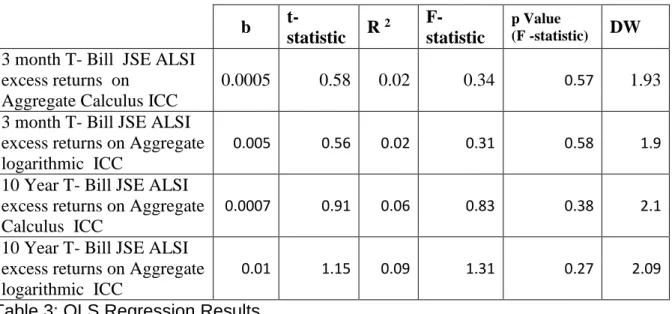
4.3 Statistical Values of Regressions This section provides the results of the regression of the excess returns with the values of the excess returns for the 3-month T Bill and the 10 Year T bill. The actual statistical values obtained from EViews are displayed in Appendix 6.
The dependent variable is the yearly market excess returns and the independent variable is the aggregate logarithmic or calculus implied cost of capital (ICC).
K is the forecasting horizon in years
b is the slope coefficient from ordinary least squares (OLS) regressions
t-statistic is the critical value obtained from ordinary least squares (OLS) regressions
R 2 is the value obtained from ordinary least squares (OLS) regressions
DW is the Durban Watson statistic which tests for autocorrelation in the residuals. A value of 2 means there is no autocorrelation in the sample.
b t-statistic R 2 F-statistic p Value (F -statistic) DW
3 month T- Bill JSE ALSI excess returns on
Aggregate Calculus ICC
0.0005 0.58 0.02 0.34 0.57 1.93
3 month T- Bill JSE ALSI excess returns on Aggregate logarithmic ICC
0.005 0.56 0.02 0.31 0.58 1.9
10 Year T- Bill JSE ALSI excess returns on Aggregate Calculus ICC
0.0007 0.91 0.06 0.83 0.38 2.1
10 Year T- Bill JSE ALSI excess returns on Aggregate logarithmic ICC
0.01 1.15 0.09 1.31 0.27 2.09
Table 3: OLS Regression Results
Calculus ICC on 3-month T Bill Excess Returns The above table 3 shows that the Implied Cost of Capital derived from the Calculus
methodology explains only 2 % of the excess returns on the JSE.
Logarithmic ICC on 3- month T Bill Excess Returns Table 3 above shows that the Implied Cost of Capital derived from the logarithmic
36
Excess Returns on 10 Year T bill The above results show that the Implied Cost of Capital derived from the Calculus
methodology explains only 5.5 % of the excess returns on the JSE.
The above results show that the Implied Cost of Capital derived from the Logarithmic derivation of ICC explains 8.5% of the excess returns on the JSE.
Our results for the logarithmic ICC give us a high interpretation of the 10 Year T Bill excess returns. So we go ahead to analyse the Serial Autocorrelation, Co-integration and Granger Causality of the Excess returns and the ICC.
F- statistic The F-statistic values obtained in table 3 above show that we can accept the null that
the excess returns follow an intercept only model. The critical F values at the 5% significance level and 1% are 1.93 and 2.5 respectively. The F static obtained for the 10 Year T bill excess returns is way less than the critical values and hence we
accept the Null that the excess returns are not well explained by the aggregate ICC values.
4.4 Validity of the Results Testing for Autocorrelation
The Breusch Godfrey test shows that we have insufficient evidence to reject the Null Hypothesis of no autocorrelation which means there is no autocorrelation at two lags (Breusch, 1978).
Testing for Co-integration Lastly after obtaining our results we tested for co-integration between the excess
returns and the Aggregate ICC. Co-integration analysis is used to determine the long term relationship between the Implied Cost of Capital and the stock market. The results in Appendix 3 from the Johansen Co-Integration Test (Johansen, 1991) show that there is no co-integration between the 10-year T Bill Excess Returns and the logarithmic ICC at the 5% significance level.
Granger Causality The Granger Causality Analysis is carried out on the 2nd lag based on the results
from the Akaike and Schwarz Information Criterion in Appendix 3 which shows that the excess returns are an AR (2) modelled process.
37
The results in Appendix 3 show that the Implied ICC does not Granger Cause the Excess Returns. Hence we can conclude that the Aggregate ICC is a good predictor of the excess returns since it is an independent source of interpreting the excess returns.
4.5 Standard Forecasting Regression Methodology
The estimation period used in the study is 2001 to 2010 to give the basis for forecasting.
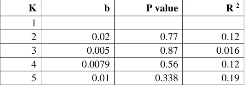
The theoretical forecast is then done at One year intervals from 2011 and the results are summarised in table 4 below. The forecasting graphs for the interval described are in Appendix 7.
The table below summarises the critical values for the different forecast horizons K is the forecasting horizon in years
b is the slope coefficient from ordinary least squares (OLS) regressions P value obtained from ordinary least squares (OLS) regressions
R 2 is the value obtained from ordinary least squares (OLS) regressions
The tables below show the outcome for the different forecast horizons: Table 4 Forecasting Critical values.
K b P value R 2 1 2 0.02 0.77 0.12 3 0.005 0.87 0.016 4 0.0079 0.56 0.12 5 0.01 0.338 0.19
The forecasting results advise us that the aggregate ICC has low explanatory power increases from 12% to 19 % in the long term. The results show that if a longer forecast horizon was taken. The ICC could be used to predict returns in the long run.
38
4.6 Discussion of Results The results obtained during the research are significant. They give us good
confidence that the ICC can be effectively used to forecast returns on the JSE. The explanatory power given by the Aggregate ICC of 9% is reasonably in line with findings by (Strydom, 2016) which shows that policy makers and investors can use CAY to predict future business returns and minimise economic downturn and losses on investments by explaining 8% of one-quarter ahead returns. However, the
Aggregate ICC offers a higher explanatory power compared to other variables which have been used on the JSE. The study by (Gupta & Modise, 2011) using
macroeconomic variables to forecast returns on the JSE also shows low explanatory power, using the R2 coefficient. The term spread could explain only approximately 4% of the variation in returns in one-quarter ahead. In the same study Treasury bill yield, could explain only 6% of the one-quarter ahead variation in returns and this value declined as the forecast horizon increased.
The standard forecasting regression methods give a different opinion of the forecasting power of the Aggregate ICC over the different horizons. In the short term horizon of one and two-year ahead forecasts, the Aggregate ICC has very low R2 values of 17 and 27%. However, the R2 values increase from the three year ahead forecast towards the five year ahead forecasts, although the ICC still explains less than 50% of the returns.
The ability of the ICC to forecast returns can further be investigated by also employing other methods of constructing the ICC. In this study the two methods used to calculate the ICC were based on the same underlying value of future earnings forecast. If a more reliable base method of deriving the base earnings per share is used, the results can yield higher explanatory power.
39
5.0 Conclusion We conclude that the Aggregate ICC cannot be used as a proxy to predict the
excess returns on the JSE for the short horizon. Although the ICC has a higher explanatory power in comparison to other proxies which have been used to predict the returns on the JSE, the coefficients of the regressions are not significant. Hence we conclude that there is not enough test data to prove the use of the ICC as a proxy for excess returns on the JSE. There is room for further study on the use of the ICC to predict returns by using different methodologies for forecasting earnings as well as calculating the ICC.
40
APPENDIX 1: Stationarity Tests
APPENDIX 2: Normality Tests
Excess Returns have a normal distribution
0 1 2 3 4 5 -0.5 -0.4 -0.3 -0.2 -0.1 0.0 0.1 0.2 0.3 Series: Residuals Sample 2000 2015 Observations 16 Mean 1.73e-17 Median 0.028065 Maximum 0.262626 Minimum -0.411119 Std. Dev. 0.172267 Skewness -0.826246 Kurtosis 3.334249 Jarque-Bera 1.894969 Probability 0.387715
41
APPENDIX 3: Validity of the Results
Serial Autocorrelation
Breusch-Godfrey Serial Correlation LM Test:
F-statistic 0.302816 Prob. F(2,12) 0.7442 Obs*R-squared 0.768713 Prob. Chi-Square(2) 0.6809
Test Equation:
Dependent Variable: RESID Method: Least Squares Date: 03/28/17 Time: 21:52 Sample: 2000 2015
Included observations: 16
Presample missing value lagged residuals set to zero.
Variable Coefficient Std. Error t-Statistic Prob.
C -0.006945 0.062065 -0.111895 0.9128 LOGARITHMIC_ICC -0.001731 0.009730 -0.177861 0.8618 RESID(-1) -0.093528 0.286239 -0.326746 0.7495 RESID(-2) -0.212273 0.289096 -0.734266 0.4769
R-squared 0.048045 Mean dependent var 1.73E-17 Adjusted R-squared -0.189944 S.D. dependent var 0.172267 S.E. of regression 0.187916 Akaike info criterion -0.293320 Sum squared resid 0.423751 Schwarz criterion -0.100173 Log likelihood 6.346563 Hannan-Quinn criter. -0.283430 F-statistic 0.201877 Durbin-Watson stat 2.067168 Prob(F-statistic) 0.893095
42 Granger Causality Tests
Pairwise Granger Causality Tests Date: 03/28/17 Time: 17:23 Sample: 2000 2015
Lags: 12
Null Hypothesis: Obs F-Statistic Prob.
LOGARITHMIC_ICC does not Granger Cause
_10_YEAR_T_BILL_EXCESS_R 4 NA NA
_10_YEAR_T_BILL_EXCESS_R does not Granger Cause LOGARITHMIC_ICC NA NA
43 APPENDIX 5: Standard Regression Outputs
Time
Year
Price
dt lo
g div
iden
ds
FE
dt-Pt
ρ
k
1-ρ
e^j
Δ
dt+j+1
mid te
rm
Sum
ICC
FY
200
0
0
13.9
00
-0.95
809
0.25
17.32
146
FY
200
1
1
15.7
41
-1.12
861
0.323
545
-16.8
693
1
3.66E
-07
-1
1.284
02541
7
-32.4
738
-41.6
97131
63
-41.6
97131
63
30.36
02472
8
FY
200
2
2
15.1
87
-1.23
385
0.371
07
-16.4
207
1
-3.7E
-08
-1
1.284
02541
7
-21.5
2
-27.6
32238
02
-69.3
29369
64
42.14
67399
9
FY
200
3
3
22.0
00
0
0.460
978
-21.9
996
1
-0.66
667
-1
1.284
02541
7
0
0
-69.3
29369
64
53.29
22117
1
FY
200
4
4
24.2
78
-1.53
161
0.584
539
-25.8
095
1
0
-1
1.284
02541
7
0
0
-69.3
29369
64
66.33
52174
4
FY
200
5
5
34.7
24
-0.90
518
0.758
086
-35.6
287
1
-0.8
-1
1.284
02541
7
323.0
827
414.8
46371
1
345.5
17001
4
-227.1
02865
2
FY
200
6
6
50.3
98
-0.78