A19/B6: A NEW LANCZOS-TYPE ALGORITHM AND ITS
IMPLEMENTATION
ZAKIR ULLAH1, MUHAMMAD FAROOQ2 AND ABDELLAH SALHI3
Abstract. Lanczos-type algorithms are mostly derived using recur-rence relationships between formal orthogonal polynomials. Various recurrence relations between these polynomials can be used for this purpose. In this paper, we discuss recurrence relationsA19andB6for the choiceUi(x) =P
(1)
i (x), whereUi is an auxiliary family of
poly-nomials of exact degreei. This leads to new Lanczos-type algorithm A19/B6that shows superior stability when compared to existing algo-rithms of the same type. This new algorithm is derived and described here. Computational results obtained with it are compared to those of the most robust algorithms of this type namelyA12,Anew12 A5/B10 andA8/B10 on the same test problems. These results are included.
Key words : Lanczos algorithm; Systems of Linear Equations;
For-mal Orthogonal Polynomials
AMS SUBJECT: Primary 65F10.
1. Introduction
In 1950, the Lanczos algorithm, [26, 13], has been introduced to cal-culate the eigenvalues of a matrix. However, it has later been adapted for the solution of systems of linear equations (SLEs) where it is now a well established solver. The Lanczos method is an iterative process which, in exact arithmetic, gives the exact solution in at mostn number
1Department of Mathematics, University of Peshawar, Khyber Pakhtunkhwa, 25120, Pakistan. Email: [email protected]
2Department of Mathematics, University of Peshawar, Khyber Pakhtunkhwa, 25120, Pakistan. Email: [email protected]
3Department of Mathematical Sciences, University of Essex, Wivenhoe Park, Colch-ester, CO4 3SQ, UK. E-mail: [email protected].
of steps [27], where n is the dimension of the problem. Several Lanczos-type algorithms have been designed and among them, the famous con-jugate gradient algorithm of Hestenes and Stiefel [25], when the matrix is Hermitian and the bi-conjugate gradient algorithm of Fletcher [22], in the general case. In the last few decades, Lanczos-type algorithms have evolved and different variants have been derived, which can be found in [2, 3, 5, 7, 10, 11, 12, 9, 14, 23, 24, 28, 29, 30, 31, 34, 35, 17].
Lanczos-type algorithms are commonly derived using Formal Orthogo-nal Polynomials (FOP’s), [5]. The connection between the Lanczos algo-rithm, [27] and orthogonal polynomials, [32] has been studied extensively in [2, 4, 5, 11, 12, 6, 8, 9, 16].
In this paper we will briefly recall recurrence relation A19 [17] for the
choice of auxiliary polynomialUi(x) =xi, wherexi is a monic polynomial
of degree i. Then we will derive expressions for the coefficients of this polynomial for a new choice ofUi(x) = P
(1)
i (x) which was not considered
before. We will also recall B6 [1] for the same choice of Ui(x). We use
the new choice ofA19 in combination ofB6 to derive a new Lanczos-type
algorithm A19/B6. This algorithm is then applied to some problems
considered in [17, 1, 33], and its performance is compared with that of existing algorithms of the same type namely A12, Anew12 A5/B10 and
A8/B10, [2, 17, 33]. The paper is organized as follows. In section 2 we will
explain the basic Lanczos process. In section 3 we will discuss the notion of FOPs. RelationsA19 andB6 are recalled in section 4. A conclusion is
given in section 5.
1.1. The Lanczos Process. Consider the following system of linear equations,
Ax=b, (1)
The basic Lanczos approach for solving SLEs (1), can be explained as follows.
Choose x0 and y, two arbitrary vectors in Rn, such that y6= 0, then
Lanczos process [27] consists in generating a sequence of vectorsxk ∈Rn,
such that
(xk−x0)∈Fk(A,r0) = span(r0,Ar0, . . . ,Ak−1r0), (2)
and
rk = (b−Axk)⊥Ek(AT,y) = span(y,ATy, . . . ,(AT)k−1y), (3)
Equation (2) implies
xk−x0 =−β1r0 −β2Ar0− · · · −βkAk−1r0. (4)
Multiplying both sides of (4) byAthen adding and subtractingbon the left hand side of (4) gives
rk =r0 +β1Ar0 +β2A2r0+· · ·+βkAkr0. (5)
If we set
Pk(x) = 1 +β1x+...+βkxk, (6)
then we can write from (5)
rk=Pk(A)r0. (7)
The polynomials Pk are known as residual polynomials [5]. Another
interpretation of thePkcan be found in [15]. From (3), the orthogonality
condition implies ((AT)iy,r
k) = (y,Airk) = (y,AiPk(A)r0) = 0, for i= 0, ..., k−1.
Thus, the coefficientsβ1,...,βk form a solution of the following system of
linear equations β1(y,Ar0) +· · ·+βk(y,Akr0) = −(y,r0), .. .
β1((AT)k−1y,Ar0) +· · ·+βk((AT)k−1y,Akr0) = −((AT)k−1y,r0).
(8)
The scalar products involved in the above system is defined as with the first argument conjugated. If the determinant of the above system is not zero then its solution exists, and thus we can obtain xk and rk from (4)
and (7) respectively. Obviously, in practice, solving the above system directly for increasing values of k is not viable; k is the order of the iterate in the solution process. Now we shall see how to solve the system (8) for increasing value of k, that is, if polynomialsPk can be computed
recursively.
Now, let ci be defined as
ci = ((AT)iy,r0) = (y, Air0), for i= 1,2, . . . ,
and the linear functionalc on the space of polynomials be given by
c(xi) =ci, for i= 0,1. . . , (9)
so the system (8) can be written as
These conditions show that Pk is a polynomial of degree at most k,
corresponding to the linear functionalcand normalized by the condition
Pk(0) = 1. Using normalization condition Pk(0) = 1, equation (6) can
be written as
Pk(x) = 1 +xQk−1(x),
whereQk−1 =β1+β2x+...+βkxk−1. Replacingx byA and multiplying
both sides by r0 we get
Pk(A)r0 =r0+AQk−1(A)r0.
Now using (7) the above relation becomes rk =r0+AQk−1(A)r0,
which can also be written as
b−Axk =b−Ax0+AQk−1(A)r0.
Simplifying and multiplying by −A−1 on both sides of the last relation,
we get
xk =x0−Qk−1(A)r0,
which shows that xk can be computed from rk recursively without
in-vertingA.
1.2. Formal Orthogonal Polynomials. The polynomial Pk(x)
dis-cussed in the previous section is defined by the following formula [5, 6, 11, 9, 12], Pk(x) = 1 x · · · xk c0 c1 · · · ck .. . ... ... ck−1 ck · · · c2k−1 Hk(1) , (11)
whereHk(1) is called the Hankel determinant [5], which is the determinant of the system (8). This determinant has the following expression:
H(1)k = c1 c2 · · · ck c2 c3 · · · ck+1 .. . ... ... ck ck+1 · · · c2k−1 .
Clearly,Pk exists if and only if H
(1)
k 6= 0. We assume in the following
sections that for all k, Hk(1) 6= 0. If for some k, Hk(1) ≈ 0, then Pk does
not exist, and breakdown occurs in the solution process. This breakdown issue is discussed elsewhere, [2, 17, 33].
Let us now define the family of orthogonal polynomialsPk(1)(x) corre-sponding to the linear functionalc(1) wherec(1) is define by
c(1)(xi) =c(xi+1) =ci+1, for i= 0,1, . . . .
These polynomials are normalized by the condition that they are monic [5, 6, 11] and are given by the following formula
Pk(1)(x) = c1 · · · ck+1 .. . ... ck · · · c2k 1 · · · xk Hk(1) . (12)
The necessary and sufficient condition for the existence and uniqueness of Pk(1)(x) is that the Hankel determinant, [5, 6, 11], is different from zero, which is the same condition as for the existence of the polynomial
Pk(x).
2. Relations A19 and B6
In the following we will recall relationsA19[17, 18] andB6 [1, 2] for the
choice of auxiliary polynomialUi(x) =xi, wherexi is a monic polynomial
of degree i. Then we will derive expressions for the coefficients of these polynomials for the choice of Ui(x) = P
(1)
i (x) which was not considered
before for relationA19. We use the new choice ofA19in tandem with B6
to derive a new Lanczos-type algorithm which we call A19/B6.
2.1. Relation A19. Consider the following recurrence relation
investi-gated in [17] Pk(x) = (Akx2+Bkx+Ck)P (1) k−2(x) + (Dkx+Ek)Pk−1(x), (13) where Pk, P (1)
k−2 and Pk−1 are polynomials of degree k, k −2 and k−1
respectively and Ak,Bk, Ck,Dk and Ek are constants to be determined
using the normalization condition ∀k, Pk(0) = 1 and orthogonality
con-ditions (C1) and (C2) given below
∀i= 0,1,· · ·k−1, c(1)(U
iP
(1)
k ) = 0 −→(C2).
Using the normalization condition, equation (13) gives 1 = Ek+CkP
(1)
k−2(0). (14)
Multiplying (13) by Ui, a polynomial of exact degree i and applying ‘c’
on both sides we get
c(UiPk) =Akc(x2UiPk(1)−2) +Bkc(xUiP (1) k−2) +Ckc(UiP (1) k−2) +Dkc(xUiPk−1) +Ekc(UiPk−1). (15) Similarly, using (C1), equation (15) becomes
Akc(x2UiP (1) k−2) +Bkc(xUiP (1) k−2) +Ckc(UiP (1) k−2) +Dkc(xUiPk−1) +Ekc(UiPk−1) = 0. (16) Fori= 0, equation (16) becomesCkc(U0P
(1)
k−2) = 0. Sincec(U0P (1)
k−2)6= 0,
therefore, Ck = 0. Hence from (14), we get Ek = 1. The orthogonality
condition (C1) is true for ∀i = 1,2,3,· · · , k −4. For i = k −3,
equa-tion (16) becomes Akc(x2Uk−3P (1)
k−2) = 0. This implies that Ak = 0 as
c(x2Uk−3P (1)
k−2)6= 0. For i=k−2, equation (16) gives
Bkc(1)(Uk−2P (1)
k−2) +Dkc(xUk−2Pk−1) = 0. (17)
Fori=k−1, equation (16) gives
Bkc(1)(Uk−1P (1) k−2) +Dkc(xUk−1Pk−1) =−c(Uk−1Pk−1). (18) If we seta11=c(1)(Uk−2P (1) k−2),a12=c(xUk−2Pk−1),a21 =c (1)(U k−1P (1) k−2),
a22=c(xUk−1Pk−1),b1 = 0, and b2 =−c(Uk−1Pk−1) then equations (17)
and (18) can be written as
a11Bk+a12Dk= 0, (19)
a21Bk+a22Dk =b2, (20)
respectively. If ∆k is the determinant of the coefficient matrix of the
above system then, ∆k =a11a22−a21a12. If ∆k 6= 0 then Bk =−b2∆ka12,
Dk = a∆k11b2. Hence,
Pk(x) =BkxP
(1)
k−2(x) + (Dkx+ 1)Pk−1(x). (21)
Let us apply the recursive formula (21) for computing polynomials Pk
replace x by A and multiply both sides by r0. Using rk = Pk(A)r0 and zk=P (1) k (A)r0, we get rk =BkAzk−2+DkArk−1 +rk−1. (22) Sincerk=b−Axk, (22) becomes b−Axk =BkAzk−2+DkArk−1+b−Axk−1.
Multiplying this latter equation byA−1 on both sides results in
xk =xk−1−Bkzk−2 −Dkrk−1, (23)
where coefficientsBkandDkcan be identified asBk=−b2∆a12
k ,Dk=
a11b2
∆k ,
respectively. So, now we choose the polynomialUi(x).
2.1.1. Case-I: When Ui(x) = xi. In the previous section we discussedA19
for general auxiliary polynomial Ui. Here we recall from [17] briefly the
same relationA19by takingUi =xi. In [17] we have ∆k=a11a22−a21a12,
where a11 = c(1)(xk−2P (1) k−2), a12 = c(xk−1Pk−1), a21 = c(1)(xk−1P (1) k−2), a22 = c(xkPk−1), b1 = 0, and b2 = −c(xk−1Pk−1). If ∆k 6= 0 then
coefficients Bk and Dk appearing in (21) are as above. Since we know
that c(xkP
k) = ((AT)ky, Pk(A)r0) = (yk,rk) and
c(xkP(1) k ) = ((A T )ky, P(1) k (A)r0) = (yk,zk), with yk=ATyk−1, (24)
using (24), we can writea11=c(1)(xk−2P (1) k−2) = (yk−1,zk−2), a12=c(xk−1Pk−1) = (yk−1,rk−1), a21=c(1)(xk−1P (1) k−2) = (yk,zk−2), a22=c(xkPk−1) = (yk,rk−1),b1 = 0, and b2 =−c(xk−1Pk−1) = −(yk−1,rk−1).
Now, since all of the above relations are only valid fork≥3, to evaluate (22) and (23) recursively, we need to evaluate r1, r2, x1, x2, z1 and z2,
which are necessary, differently. These values are determined in detail in [1, 17]. They are recalled briefly here, however, for completeness, as follows.
r1 =r0−(cc01)Ar0, x1 =x0+ (cc01)r0 where ci = (y,Air0),
r2 =r0−αAr0+βA2r0,x2 =x0 +αr0−βAr0,
z1 =Ar0−(cc21)r0, z2 =A2r0−α1Ar0+β1r0.
whereδ =c1c3−c22, α= c0c3−c1c2 δ , β = c0c2−c21 δ ,δ1 =c1c3−c 2 2, α1 = c1c4δ−c2c3 1 , and β1 = c2c4−c23 δ1 . 2.1.2. Case-II: When Ui(x) = P (1)
i (x). In this section, we derive A19
for a different choice of Ui(x) which was not considered before. All the
coefficients involved inA19 have completely different expressions for this
new choice of Ui(x) as explained below. For Ui(x) = P
(1)
i (x) all of the
above expressions will have the following form:
a11=c(1)(P (1) k−2P (1) k−2),a12=c(xP (1) k−2Pk−1), a21 =c(1)(P (1) k−1P (1) k−2), a22=c(xP (1) k−1Pk−1),b1 = 0, and b2 =−c(P (1) k−1Pk−1). Using c(1)(P(1) k−1P (1) k−2) = 0, zk =P (1) k (A)r0, ˜zk =P (1) k (A T)˜z 0, rk=Pk(A)r0, and c(UkPk) = (y, Uk(A)Pk(A)r0) = (Uk(AT)y, Pk(A)r0) = (˜zk, rk) [notez˜0 =y], (25) we geta21= 0,a11 =c(1)(Pk(1)−2P (1) k−2) = (˜zk−2, Azk−2),a12=c(xP (1) k−2Pk−1) = (˜zk−2, Ark−1), a22 = c(xP (1) k−1Pk−1) = (˜zk−1, Ark−1), b1 = 0, b2 = −c(Pk(1)−1Pk−1) = −(˜zk−1,rk−1), ∆k=a11a22, Bk =−b2∆ka12, and Dk= ab222 .
Hence, after evaluating the coefficients Ak, Bk, Ck, ∆k and Ek for the
choice Ui(x) =Pi(1)(x) equation(13) reduces to
Pk(x) =BkxP
(1)
k−2(x) + (Dkx+ 1)Pk−1(x). (26)
Replacing x by A and multiplying both sides by r0 and using rk =
Pk(A)r0, and zk=P (1) k (A)r0 we get rk =BkAzk−2+DkArk−1 +rk−1. (27) Sincerk=b−Axk, (14) becomes xk =xk−1−Bkzk−2 −Dkrk−1. (28)
2.2. Relation B6. Consider the following recurrence relation
investi-gated in [1] Pk(1)(x) = (Akx2+Bkx+Ck)P (1) k−2(x) + (Dkx+Ek)P (1) k−1(x), (29)
wherePk(1), Pk(1)−2 and Pk(1)−1 are polynomials of degree k, k−2 and k−1 respectively and Ak,Bk, Ck,Dk and Ek are constants to be determined
as already discussed in[1, 2] for the choicesxi,Pk(x),P
(1)
and recall B6 for general auxiliary polynomial Ui, a polynomial of exact
degreei. Multiply (29) by Ui and apply c(1) on both sides to get
c(1)(UiP (1) k ) = Akc(1)(x2UiP (1) k−2) +Bkc(1)(xUiP (1) k−2) +Ckc(1)(UiPk(1)−2) +Dkc (1) (xUiPk(1)−1) +Ekc (1) (UiPk(1)−1). (30) Using (C2) we get Akc(1)(x2UiP (1) k−2) +Bkc(1)(xUiP (1) k−2) +Ckc(1)(UiP (1) k−2) +Dkc(1)(xUiPk(1)−1) +Ekc (1) (UiPk(1)−1) = 0. (31) The orthogonality condition (C2) is true for ∀i= 0,1,2,· · ·k−5.
Fori=k−4, we get Akc(1)(x2Uk−4P (1)
k−2) = 0, which implies that
Ak = 0 as c(1)(x2Uk−4P (1)
k−2) 6= 0. But P (1)
k is a monic polynomial of
degreek; so Dk = 1. Fori=k−3, we getBkc(1)(xUk−3P (1) k−2) = 0. Since c(1)(xUk−3P (1) k−2)6= 0, Bk = 0. For i = k−2, we have c(1)(xUk−2Pk(1)−1) +Ckc (1)(U k−2Pk(1)−2) = 0 which implies that Ck=− c(1)(xUk−2P (1) k−1) c(1)(U k−2P (1) k−2) . (32) Fori=k−1, we get c(1)(xUk−1P (1) k−1) +Ckc(1)(Uk−1P (1) k−2) +Ekc(1)(Uk−1P (1) k−1) = 0. Sincec(1)(U k−1P (1) k−1)6= 0, Ek = −c(1)(xUk−1P (1) k−1)−Ckc(1)(Uk−1P (1) k−2) c(1)(U k−1P (1) k−1) . (33) Hence (29) becomes Pk(1)(x) = CkP (1) k−2(x) + (x+Ek)P (1) k−1(x), where Ck=− c(1)(xU k−2P (1) k−1) c(1)(U k−2Pk(1)−2) , and Ek = −c(1)(xU k−1P (1) k−1)−Ckc(1)(Uk−1P (1) k−2) c(1)(U k−1P (1) k−1) .
2.2.1. Relation B6 when Ui(x) = P
(1)
i (x). In this case, (32) and (33)
become Ck =− c(x2P(1) k−2P (1) k−1) c(xPk(1)−2Pk(1)−2),and Ek= −c(1)(xPk(1)−1P (1) k−1)−Ckc(1)(P (1) k−1P (1) k−2) c(1)(P(1) k−1P (1) k−1) , respectively. Using c(1)(P(1) k−1P (1) k−2) = 0, zk=Pk(1)(A)r0, ˜zk=Pk(1)(AT)˜z0, rk =Pk(A)r0, and c(UkPk) = (y, Uk(A)Pk(A)r0) = (Uk(AT)y, Pk(A)r0) = (˜zk, rk), [note ˜z0 =y], (34) we get Ck =− c(x2P(1) k−2P (1) k−1) c(xPk(1)−2P (1) k−2) =−(˜zk−2,A2zk−1) (˜zk−2,Azk−2), and Ek=− c(x2P(1) k−1P (1) k−1) c(xPk(1)−1Pk(1)−1) =− (˜zk−1,A2zk−1) (˜zk−1,Azk−1).
Hence after evaluating the coefficients Ak, Bk, Ck, Dk and Ek for the
choice Ui(x) =P (1) i (x) equation (29) reduces to Pk(1)(x) = CkP (1) k−2(x) + (x+Ek)P (1) k−1(x). (35)
Replacing x byA, multiplying by r0 and using zk =P
(1)
k (A)r0 we get
zk =Ckzk−2+Azk−1+Ekzk−1.
Replacing x by AT and multiply by ˜z0 = y and using ˜zk = P
(1) k (A T)˜z 0, we get ˜ zk =Ck˜zk−2+AT˜zk−1+Ek˜zk−1.
2.3. Algorithm A19/B6. We now consider the combination of A19 and
B6 for the choice Ui(x) = P
(1)
i (x) which, as said earlier, was never
con-sidered before. The new algorithm is called A19/B6 and its pseudo-code
Algorithm 1Lanczos-type Algorithm A19/B6.
1: Choose x0 and y such thaty6= 0.
2: Set r0 =b−Ax0, ˜z0 =y, 3: z0 =r0. 4: p =Ar0, p1 =Ap, p2 =Ap1, p3 =Ap2, 5: c0 = (y,r0), c1 = (y,p),c2 = (y,p1), 6: c3 = (y,p2), c4 = (y,p3),δ =c1c3−c22, 7: α = c0c3−c1c2 δ ,β = c0c2−c21 δ ,δ1 =c1c3−c 2 2, 8: α1 = c1c4δ−1c2c3,β1 = c2c4−c23 δ1 , 9: r1 =r0−(cc0 1)p, x1 =x0+ ( c0 c1)r0, 10: r2 =r0−αp+βp1, 11: x2 =x0 +αr0−βp, 12: z1 =p−(cc21)r0,z2 =p1−α1p+β1r0, 13: y1 =ATy,y 2 =ATy1, 14: z˜1 =y1−(cc21)˜z0, 15: z˜2 =y2−α1y1+β1z˜0, 16: for k=3,4,... do 17: q1 =Ark−1, q2 =Azk−1, q3 =Aq2,q4 =Azk−2, s=AT˜zk−1 18: a11=c(1)(P (1) k−2P (1) k−2) = (˜zk−2, q4) 19: a12=c(xP (1) k−2Pk−1) = (˜zk−2, q1) 20: a22=c(xP (1) k−1Pk−1) = (˜zk−1, q1) 21: b2 =−c(P (1) k−1Pk−1) = −(˜zk−1,rk−1) 22: ∆k =a11a22, 23: if ∆k≤
24: print “ghost-type breakdown”
25: stop. 26: end if 27: Bk=−b2∆ka12,Dk = ab222 28: rk=Bkq4+Dkq1+rk−1 29: xk =xk−1−Bkzk−2−Dkrk−1 30: if ||rk||> then 31: Ck =− c(x2P(1) k−2P (1) k−1) c(xPk(1)−2Pk(1)−2) =− (˜zk−2,q3) (˜zk−2,q4) 32: Ek =− c(x2P(1) k−1P (1) k−1) c(xPk(1)−1Pk(1)−1) =− (˜zk−1,q3) (˜zk−1,q2) 33: zk =Ckzk−2+q2+Ekzk−1 34: z˜k =Ck˜zk−2+s+Ek˜zk−1 35: else 36: x=xk 37: stop 38: end if 39: end for
Algorithm 1 has been implemented in Matlab and tested on the fol-lowing problem which was considered in [17, 1, 33, 21]. This problem arises in the 5-point discretisation of the operator −dxd22 −
d2 dy2 +γ
d
dx on a
rectangular region, [17, 1]. Comparative results on instances of the prob-lem Ax = b ranging from dimension 10 to 900 for parameter δ taking value 0.0 and 0.2 and for the tolerance = 10−05 are recorded in Tables
1 and 2. A= B −I · · · 0 −I B −I ... .. . . .. ... ... ... .. . −I B −I 0 · · · −I B , with B = 4 α · · · 0 β 4 α ... .. . . .. ... ... ... .. . β 4 α 0 · · · β 4 ,
andα=−1 +δ,β =−1−δ. Whenδ = 0, the matrix of coefficients A is symmetric and the problem is easy to solve. Forδ= 0.2 the matrix A is non-symmetric and the problem is comparatively harder as the region is not a regular mesh. The dimension of the matrixB= 10. The right hand side b is taken to beb=Ax, wherex= (1,1, . . . ,1)T, is the solution of the system.
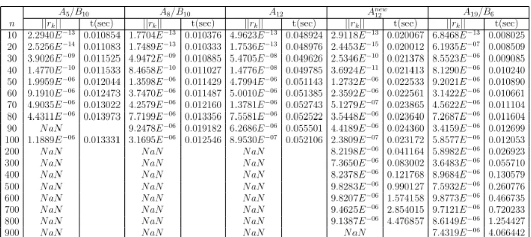
Table 1. A19/B6 versus A12, A12new, A5/B10 and A8/B10
for problems of different dimensions when δ= 0
A5/B10 A8/B10 A12 Anew12 A19/B6
n ||rk|| t(sec) ||rk|| t(sec) ||rk|| t(sec) ||rk|| t(sec) ||rk|| t(sec)
10 2.2940E−13 0.010854 1.7704E−13 0.010376 4.9623E−13 0.048924 2.9118E−13 0.020067 6.8468E−13 0.008025 20 2.5256E−14 0.011083 1.7489E−13 0.010333 1.7536E−13 0.048976 2.4453E−15 0.020012 6.1935E−07 0.008509 30 3.9026E−09 0.011525 4.9472E−09 0.010885 5.4705E−08 0.049626 2.5346E−10 0.021378 8.5523E−06 0.009085 40 1.4770E−10 0.011533 8.4658E−10 0.011027 1.4776E−08 0.049785 3.6924E−11 0.021413 8.1290E−06 0.010240 50 1.9959E−06 0.012044 1.3598E−06 0.011429 4.7994E−06 0.051143 1.2732E−06 0.022533 9.2021E−06 0.010890 60 9.1910E−06 0.012473 3.7470E−06 0.011487 5.0010E−06 0.051385 2.3592E−06 0.022561 3.1422E−06 0.010661 70 4.9035E−06 0.013022 4.2579E−06 0.012160 1.3781E−06 0.052743 5.1279E−07 0.023865 4.5622E−06 0.011104 80 4.4311E−06 0.013973 7.7199E−06 0.013356 7.5581E−06 0.052522 3.5448E−06 0.023640 7.2687E−06 0.011604 90 N aN 9.2478E−06 0.019182 6.2686E−06 0.055501 4.4189E−06 0.024360 3.4159E−06 0.012699 100 1.1889E−06 0.013331 3.1695E−06 0.012546 8.9530E−07 0.052106 2.3809E−07 0.023172 5.8577E−06 0.012053 200 N aN N aN N aN 8.2198E−06 0.041164 5.8982E−06 0.026923 300 N aN N aN N aN 7.3650E−06 0.083002 3.6483E−06 0.055710 400 N aN N aN N aN 8.2378E−06 0.121768 8.9684E−06 0.130579 500 N aN N aN N aN 9.8283E−06 0.990127 7.5932E−06 0.260776 600 N aN N aN N aN 9.8207E−06 1.574158 9.8773E−06 0.466735 700 N aN N aN N aN 9.4625E−06 2.854015 9.7121E−06 0.720233 800 N aN N aN N aN 9.1387E−06 4.476857 8.6149E−06 1.254427 900 N aN N aN N aN N aN 7.4319E−06 4.066442
The results show that forδ = 0 algorithmA19/B6 solved the given
prob-lems for dimensions up to 900 while the existing three algorithms namely
A5/B10, A8/B10 and A12 failed on systems of dimension n >100.
Table 2. A19/B6 versus A12, A12new, A5/B10 and A8/B10
for problems of different dimensions when δ= 0.2
A5/B10 A8/B10 A12 Anew12 A19/B6
n ||rk|| t(sec) ||rk|| t(sec) ||rk|| t(sec) ||rk|| t(sec) ||rk|| t(sec)
10 9.8216E−10 0.017858 2.3567E−10 0.010808 2.0583E−08 0.049232 4.7266E−08 0.021279 7.5451E−06 0.017863 20 4.1778E−11 0.011341 5.8526E−11 0.010930 6.3915E−10 0.049101 5.9892E−10 0.021293 3.7108E−06 0.020886 30 2.6438E−06 0.012366 5.9072E−06 0.012117 5.9403E−06 0.050672 6.8627E−06 0.022881 9.2819E−06 0.021169 40 N aN N aN 7.6080E−06 0.051437 7.8688E−06 0.023776 6.8914E−06 0.023724 50 N aN N aN 8.8143E−06 0.066431 5.0100E−06 0.028116 7.2611E−06 0.022813 60 N aN N aN N aN 2.6424E−06 0.024839 5.9941E−06 0.025928 70 N aN N aN N aN 9.9853E−06 0.237743 9.3422E−06 0.024190 80 N aN N aN N aN N aN 3.8215E−06 0.025606 90 N aN N aN N aN N aN 7.7488E−06 0.037380 100 N aN N aN N aN N aN 7.7186E−06 0.045345 200 N aN N aN N aN N aN 3.5339E−06 0.052006 300 N aN N aN N aN N aN 6.5440E−06 0.136388 400 N aN N aN N aN N aN 7.2847E−06 0.259785 500 N aN N aN N aN N aN 2.8823E−06 0.278282 600 N aN N aN N aN N aN 8.9049E−06 0.445157
As can be seen in Table 2, forδ = 0.2, algorithmA19/B6 solved the given
problems for dimensions up to 500 while algorithmsA5/B10, and A8/B10
failed for n= 40 and A12, Anew12 failed for n= 60 and above.
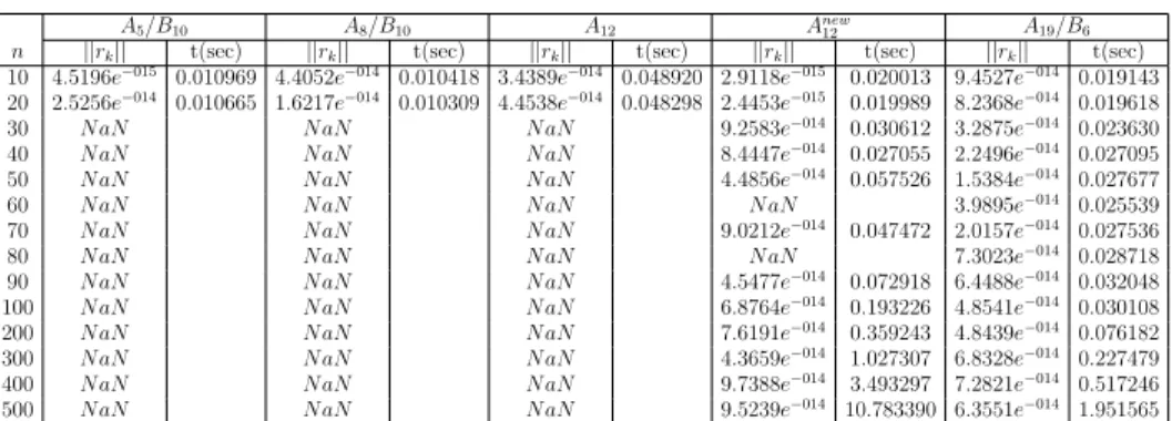
If we decrease the tolerance from 10−05 to 10−013 the numerical results are strongly in favor of A19/B6 which is clear from Table 3 and Table 4.
Table 3. A19/B6 versus A12, A12new, A5/B10 and A8/B10
for problems of different dimensions when δ= 0
A5/B10 A8/B10 A12 Anew12 A19/B6
n ||rk|| t(sec) ||rk|| t(sec) ||rk|| t(sec) ||rk|| t(sec) ||rk|| t(sec)
10 4.5196e−015 0.010969 4.4052e−014 0.010418 3.4389e−014 0.048920 2.9118e−015 0.020013 9.4527e−014 0.019143 20 2.5256e−014 0.010665 1.6217e−014 0.010309 4.4538e−014 0.048298 2.4453e−015 0.019989 8.2368e−014 0.019618 30 N aN N aN N aN 9.2583e−014 0.030612 3.2875e−014 0.023630 40 N aN N aN N aN 8.4447e−014 0.027055 2.2496e−014 0.027095 50 N aN N aN N aN 4.4856e−014 0.057526 1.5384e−014 0.027677 60 N aN N aN N aN N aN 3.9895e−014 0.025539 70 N aN N aN N aN 9.0212e−014 0.047472 2.0157e−014 0.027536 80 N aN N aN N aN N aN 7.3023e−014 0.028718 90 N aN N aN N aN 4.5477e−014 0.072918 6.4488e−014 0.032048 100 N aN N aN N aN 6.8764e−014 0.193226 4.8541e−014 0.030108 200 N aN N aN N aN 7.6191e−014 0.359243 4.8439e−014 0.076182 300 N aN N aN N aN 4.3659e−014 1.027307 6.8328e−014 0.227479 400 N aN N aN N aN 9.7388e−014 3.493297 7.2821e−014 0.517246 500 N aN N aN N aN 9.5239e−014 10.783390 6.3551e−014 1.951565
The results show that for = 10−013 and δ = 0 algorithms A
19/B6 and
Anew
12 solved the given problem for dimensions up to 500 while A5/B10,
A8/B10 and A12 failed for n = 30 and above.
Table 4. A19/B6 versus A12, A12new, A5/B10 and A8/B10
for problems of different dimensions when δ= 0.2
A5/B10 A8/B10 A12 Anew12 A19/B6
n ||rk|| t(sec) ||rk|| t(sec) ||rk|| t(sec) ||rk|| t(sec) ||rk|| t(sec)
10 1.4521E−14 0.012071 4.7905E−14 0.011465 2.9806E−14 0.050647 N aN 2.4294E−14 0.020081 20 N aN N aN N aN N aN 6.0869E−14 0.028402 30 N aN N aN N aN N aN 5.1766E−14 0.028676 40 N aN N aN N aN N aN 5.1502E−14 0.032685 50 N aN N aN N aN N aN 8.9242E−14 0.031879 60 N aN N aN N aN N aN 1.9212E−14 0.037306 70 N aN N aN N aN N aN 5.5211E−14 0.048051 80 N aN N aN N aN N aN 9.8420E−14 0.049704 90 N aN N aN N aN N aN 5.0930E−14 0.061245 100 N aN N aN N aN N aN 9.0537E−14 0.069353 200 N aN N aN N aN N aN 1.0460E−14 0.126791
Again, for = 10−013 and δ = 0.2 algorithm A
19/B6 solved the given
problems up to dimension 200 while the other algorithms failed forn= 10 and above. The obvious reason is breakdown, [19, 20]. Since all these al-gorithms consist of recursively computingPkandP
(1)
k , which involves the
calculation of some scalar products appearing as denominators and nu-merators of the coefficient of the recurrence relationships, when any of the denominators become very small, as small as, for instance 2.3879×10−014,
breakdown occurs and the algorithms fail. This breakdown issue is be-ing investigated further and any findbe-ing will be reported in forthcombe-ing papers.
According to [1, 17, 21, 33], algorithms A12, Anew12 , A5/B10 and A8/B10
are considered as the most robust Lanczos-type algorithms. We have now compared our new algorithm with these algorithms on a standard problem considered in this paper and elsewhere. Our results show that algorithm A19/B6 is faster through out, and more robust overall.
3. Conclusion
In this paper, we derived the recurrence relationA19 [17] and recalled
B6 [1] both using the general auxilliary polynomial Ui(x). We used A19
in tandem withB6 to derive a new Lanczos-type algorithmA19/B6. This
new algorithm has been applied to a number of instances of some stan-dard test problem considered in [17, 1, 33] and elsewhere. The perfor-mance of this algorithm is compared to that of existing and well es-tablished algorithms of the same type namely, A12, Anew12 , A5/B10 and
A8/B10, [2, 17, 33]. Numerical results are strongly in favour of the new
algorithm A19/B6.
References
[1] C. Baheux.Algorithmes d’implementation de la m´ethode de Lanczos. PhD thesis, University of Lille 1, France, 1994.
[2] C. Baheux. New Implementations of Lanczos Method.Journal of Computational
and Applied Mathematics, 57:3–15, 1995.
[3] A. Bjˆorck, T. Elfving, and Z. Strakos. Stability of Conjugate Gradient and Lanc-zos Methods for Linear Least Squares Problems.SIAM Journal of Matrix
Anal-ysis and Application, 19:720–736, 1998.
[4] C. Brezinski. Pad´e-Type Approximation and General Orthogonal Polynomials,
Internat. Ser. Nuner. Math. 50. Birkh¨auser, Basel, 1980.
[5] C. Brezinski and H. Sadok. Lanczos-type algorithms for solving systems of linear equations.Applied Numerical Mathematics, 11:443–473, 1993.
[6] C. Brezinski and M. R. Zaglia. A new presentation of orthogonal polynomials with applications to their computation. Numerical Algorithms, 1:207–222, 1991. [7] C. Brezinski and M. R. Zaglia. Hybird procedures for solving linear systems.
Numerische Mathematik, 67:1–19, 1994.
[8] C. Brezinski, M. R. Zaglia, and H. Sadok. Avoiding breakdown and near-breakdown in Lanczos type algorithms.Numerical Algorithms, 1:261–284, 1991. [9] C. Brezinski, M. R. Zaglia, and H. Sadok. A Breakdown-free Lanczos type
algo-rithm for solving linear systems.Numerische Mathematik, 63:29–38, 1992. [10] C. Brezinski, M. R. Zaglia, and H. Sadok. New look-ahead Lanczos-type
algo-rithms for linear systems.Numerische Mathematik, 83:53–85, 1999.
[11] C. Brezinski, M. R. Zaglia, and H. Sadok. The matrix and polynomial approaches to Lanczos-type algorithms.Journal of Computational and Applied Mathematics, 123:241–260, 2000.
[12] C. Brezinski, M. R. Zaglia, and H. Sadok. A review of formal orthogonality in Lanczos-based methods.Journal of Computational and Applied Mathematics, 140:81–98, 2002.
[13] C. G. Broyden and M. T. Vespucci.Krylov Solvers For Linear Algebraic Systems. Elsevier, Amsterdam, The Netherlands, 2004.
[14] D. Calvetti, L. Reichel, F. Sgallari, and G. Spaletta. A Regularizing Lanczos iteration method for underdetermined linear systems. Jouranl of Computational
and Applied Mathematics, 115:101–120, 2000.
[15] G. Cybenko. An explicit formula for Lanczos plonomials.Linear Algebra Appl., 88/89:99–115, 1987.
[16] A. Draux. Polynˆomes Orthogonaux Formels. Application, LNM 974. Springer-Verlag, Berlin, 1983.
[17] M. Farooq. New Lanczos-type Algorithms and their Implementation. PhD the-sis, University of Essex, UK, 2011. http://serlib0.essex.ac.uk/record= b1754556.
[18] M. Farooq and A. Salhi. New Recurrence Relationships between Orthogonal Polynomials which Lead to New Lanczos-type Algorithms. Journal of Prime
Research in Mathematics, 8:61–75, 2012.
[19] M. Farooq and A. Salhi. A Restarting Approach to Beating the Inherent Insta-bility of Lanczos-type Algorithms. Iranian Journal of Science and Technology,
Transaction A-Science, 37(3.1):349–358, 2013.
[20] M. Farooq and A. Salhi. A Switching Approach to Avoid Breakdown in Lanczos-type Algorithms. Applied Mathematics and Information Sciences, 8(5):2161– 2169, 2014.
[21] M. Farooq and A. Salhi. A new Lanczos-type algorithm for system of linear equations.Journal of Prime Research in Mathematics, 10:116–121, 2015. [22] R. Fletcher. Conjugate Gradient methods for indefinite systems. In G.A. Watson,
editor,Numerical Analysis, Dundee 1975, Lecture Notes in Mathematics,, volume 506. Springer, Berlin, 1976.
[23] A. Greenbaum.Iterative Methods for Solving Linear System. Society for Indus-trial and Applied Mathematics, Philadelphia, 1997.
[24] A. El Guennouni. A unified approach to some strategies for the treatment of breakdown in Lanczos-type algorithms.Applicationes Mathematicae, 26:477–488, 1999.
[25] M. R. Hestenes and E. Stiefel. Mehtods of Conjugate Gradients for solving linear systems.Journal of the National Bureau of Standards, 49:409–436, 1952. [26] C. Lanczos. An Iteration Method for the Solution of the Eigenvalue Problem of
Linear Differential and Integeral Operators.Journal of Research of the National
Bureau of Standards, 45:255–282, 1950.
[27] C. Lanczos. Solution of systems of linear equations by minimized iteration.
Jour-nal of the NatioJour-nal Bureau of Standards, 49:33–53, 1952.
[28] G. Meurant.The Lanczos and Conjugate Gradient algorithms, From Theory to
Finite Precision Computations. SIAM, Philadelphia,2006.
[29] B. N. Parlett and D. S. Scott. The Lanczos Algorithm With Selective Orthogo-naliztion.Mathematics of Computation, 33:217–238, 1979.
[30] B. N. Parlett, D. R. Taylor, and Z. A. Liu. A Look-Ahead Lanczos Algorithm for Unsymmetric Matrices. Mathematics of Computation, 44:105–124, 1985. [31] Y. Saad. On the Lanczos method for solving linear system with several right-hand
sides.Mathematics of Computation, 48:651–662, 1987.
[32] G. Szeg¨o.Orthogonal Polynomials. American Mathematical Society, Providence, Rhode Island, 1939.
[33] S. Ullah, M. Farooq, and A. Salhi. An alternative derivation of a new Lanczos-type algorithm for systems of linear equations. Punjab University Journal of
Mathematics, 45:39–49, 2013.
[34] H. A. Van Der Vorst. An iterative solution method for solving f(A)x=b, using Krylov subspace information obtained for the symmetric positive definite matrix
A. Journal of Computational and Applied Mathematics, 18(2):249–263, 1987.
[35] Q. Ye. A Breakdown-Free Variation of the Nonsymmetric Lanczos Algorithms.