Nonparametric Estimation of Transition Probabilities for a General Progressive
Multi-State Model Under Cross-Sectional Sampling
Jacobo de U˜na- ´Alvarez
Department of Statistics and OR and Center for Biomedical Research (CINBIO), University of Vigo, Vigo 36310, Spain.
email:[email protected] and
Micha Mandel
Department of Statistics, The Hebrew University of Jerusalem, Jerusalem 91905, Israel. email:[email protected]
Summary: Nonparametric estimation of the transition probability matrix of a progressive multi-state model is
considered under cross-sectional sampling. Two different estimators adapted to possibly right-censored and left-truncated data are proposed. The estimators require full retrospective information before the truncation time, and are obtained as differences between two survival functions constructed for sub-samples of subjects occupying specific states at a certain time point. Both estimators correct the oversampling of relatively large survival times by using the left-truncation times associated with the cross-sectional observation. Asymptotic results are established, and finite sample performance is investigated through simulations. One of the proposed estimators performs better when there is no censoring, while the second one is strongly recommended with censored data. The new estimators are applied to data on patients in intensive care units (ICUs).
Key words: Biased data; Illness-Death Model; Inverse weighting; Left truncation; Multi-state models.
1. Introduction
Multi-state models are often used to represent and to investigate the evolution of a disease over time. For this, several relevant transient states like ‘healthy’, ‘diseased’ and so on are typically identified, together with one or more absorbing states (‘dead’, ‘discharged’ etc). Emphasis often lies on estimation of the so-called transition probabilities, which allow for long-term survival prognosis (Hougaard, 2000). The transition probabilities evaluate the probability of occupying a particular state at some future time, given the current state of the process. The model is said to fulfill the Markov assumption when these probabilities are independent of the states previously visited by the process and the transition times among them. The standard nonparametric estimator for a Markovian transition probability matrix from possibly right-censored data is the time-honored Aalen-Johansen estimator (Aalen and Johansen, 1978). This estimator is easily adapted to the left-truncated case by a suitable modification of the risk sets (Andersen et al., 1993). Although the Aalen-Johansen estimator serves to consistently estimate the occupation probabilities regardless of the Markov condition (Datta and Satten 2001), it may be systematically biased when the goal is to estimate the transition probability matrix and the Markov condition is violated (Meira-Machado et al., 2006).
In a recent paper, de U˜na- ´Alvarez and Meira-Machado (2015) compared several nonpara-metric estimators for the transition probability matrix of a possibly non-Markov, censored progressive illness-death model; see also Balboa and de U˜na- ´Alvarez (2017). The estimator showing the best performance was a Pepe-type estimator (Pepe, 1991), defined as a difference of two Kaplan-Meier survival estimators of particular event times, computed from specific subsamples. These authors discussed ways to apply the subsampling approach to a completely general progressive multi-state model. The idea of subsampling proceeds by evaluating the transition probabilities from the subset of individuals observed at the state of interest by
the given time. This resembles the idea of landmarking, as described in van Houwelingen and Putter (2012); see also Putter and Spitoni (2016) who introduced the landmark Aalen-Johansen estimator and proved that it is consistent for censored, non-Markov processes. A related piece of work was independently built up by Titman (2015), who considered multi-state models that are possibly non-progressive.
In biomedical research, cross-sectional samplings or prevalence studies are often applied due to their simplicity relative to incidence (prospective) designs. Cross-sectional data refer to individuals ‘in progress’ (i.e. alive) by the sampling date; thus, the individual survival times are left-truncated by the recruitment times. An example, further studies in Section 4, is a study on intensive care units (ICUs) conducted during 1999 and 2000 in Israel. Five hospitals were cross-sectioned on four independent days in order to identify patients who met pre-specified ICU criteria. Information on patients was gathered from the day of deterioration, i.e., the day when the patient first met the ICU criteria, to 30 days afterward. The main interest was to estimate the probability of acquiring a bloodstream infection (BSI), a severe infection that is one of the leading causes of death inside hospitals. Thus, the process has two transient states: 1-hospitalized without BSI and 2 - hospitalized with BSI; and two absorbing states: 3 - discharged alive from the ICU and 4 - died in the ICU.
Under cros-sectional sampling, standard estimation procedures must be corrected for the oversampling of individuals with a relatively large survival times. Although several authors study nonparametric estimation from multi-state cross-sectional data (Chang and Tzeng, 2006; Mandel, 2010; Vakulenko-Lagun et al., 2017), they do not focus on estimation of transition probabilities with full generality or they impose distributional assumptions on the truncating variable; see also the discussion in Section 5. For non-Markov processes, Allignol et al. (2014) and Titman (2015) consider the issue of left-truncation in a setting in which the individual trajectory prior to the truncation time is not available. In cases when
retrospective information is available, these latter methods ignore data on states visited before the cross-section date, thus resulting in a potential loss of efficiency. In the ICU data and similar data collected in hospitals, patients are closely monitored and full history information before truncation is available. The purpose of the current paper is to introduce and to investigate nonparametric estimators for the transition probability matrix in a general, progressive multi-state model from cross-sectional (possibly censored) data, making use of the available retrospective information. Neither the Markov condition, nor distributional assumptions on the truncation time, will be imposed.
The rest of the paper is organized as follows. In Section 2 we introduce the needed notations, the estimators and the main results. In Section 3 we conduct a simulation study to compare the two proposed estimators. An application to the study of hospitalization time in an ICU is given in Section 4. The main conclusions and a final discussion are deferred to Section 5.
2. Notations, estimators and main results
2.1 Model
Consider a progressive multi-state process formed by transient and absorbing states; each state can be visited once at maximum. Let X(t) denote the state occupied by the process at time t, t > 0. Let T0 denote the total survival time or absorption time, that is, the
time up to reaching one of the absorbing states. For a given state j, let Ej denote the set
of states from which j is reachable. Let Z0,j and T0,j denote the sojourn times in Ej and
Ej∪ {j}respectively. When Ej is empty, we set Z0,j = 0 by convention. Note that the event
{X(t) = j} can be written as {Z0,j 6 t < T0,j} and, therefore, the occupation probability
for state j satisfies
P(X(t) =j) =P(T0,j > t)−P(Z0,j > t). (1)
survival functions corresponding to the sojourn times Z0,j andT0,j. Ifj is the only absorbing state of the process, then P(T0,j = ∞) = 1, Z0,j = T0, and P(X(t) = j) = 1−P(T0 > t) is the cumulative distribution function of the absorption time T0 at time t. If j is one among several absorbing states, we rather get from (1) a cumulative incidence function,
P(X(t) =j) = P(Z0,j 6t, νj = 1), whereνj stands for the indicator of visiting statej. Since
Z0,j equals T0 in the presence of νj = 1, one may write P(X(t) = j) = P(T0 6 t, νj = 1); that is, the occupation probability equals the cumulative incidence function of T0 for the event ‘reaching the absorbing state j’.
Similar formulae can be derived for the transition probabilities of the process, which are defined as
pij(s, t) =P(X(t) =j | X(s) =i),
where i, j are states and s, t are time points with s < t. Explicitly, when j is transient we will refer to
pij(s, t) = P(T0,j > t| X(s) =i)−P(Z0,j > t| X(s) =i), (2)
while when j is absorbing we will rather use
pij(s, t) =P(T0 6t, νj = 1 | X(s) = i). (3)
Under cross-sectional sampling, an individual is observed if and only if L 6 T0, where L
denotes the time from onset to cross-section, and plays the role of left-truncation time. For simplicity, we assume that the lower limit of the support of L, aL say, is zero; note
that, in general, with left-truncated data one can only identify the conditional distribution of T0 given T0
> aL. Furthermore, there is in general some risk of right-censoring after
recruitment. Let C denote the potential censoring time, with P(C > L) = 1; so rather than (L, T0) with L
6 T0 one observes (L, T,∆) with L
6 T, where T = min(T0, C) and
is fully available, including the states visited before recruitment and the transition times among them. This is in contrast to the more standard left-truncated scenario with event history data, in which information on the individual is restricted to the follow-up after the date of sampling (Andersen et al., 1993). In our context, the data at hand are iid copies of (L, Zj, δj, Tj,δ˜j, T,∆) conditionally on L 6 T, for the various states j of the process. Here Zj and δj (Tj and ˜δj) denote the possibly censored sojourn time in Ej (Ej ∪ {j})
and its censoring indicator. Note that ∆ = 1 (uncensored trajectory of the process) implies
δj = 1 for each j. In the case ∆ = 1, the absorbing state reached by the individual is also observed. Our goal is to nonparametrically estimate the transition probabilities from such left-truncated and right-censored sojourn times on the basis of equations (2) and (3).
We assume that the pair (L, C) is independent of the process of interest, as is usual with left-truncated and right-censored data. This independence assumption just means that the cross-sectional sampling and the follow-up of the individuals are unrelated to the process under investigation. However, we allow C and L to be dependent; indeed, under cross-sectional sampling, L and C are correlated due to the restriction P(C > L) = 1. The two estimators we propose below for pij(s, t) are computed from a specific subsample, S
(s)
i ,
determined by the state i and the time point s. Explicitly, Si(s) denotes the subsample of individuals observed in state i by times, that is, the ones satisfying the condition{X(s) =
i, C > s}. Note that the independence between (L, C) and the process remains in such
subpopulation. This ensures the consistency of the methods.
2.2 Product-limit integral type estimator
The first estimator we propose is a combination of special product-limit integrals as those considered by S´anchez-Sellero, Gonz´alez-Manteiga, and Van Keilegom (2005). Specifically, let Z0 denote either Z0,j or T0,j in (2), and let Z = min(Z0, C) be the observable version of
Z0. Then, the joint distribution function of (Z0, T0) can be estimated from the left-truncated
and right-censored data by (see Web Appendix A) ˆ FZ0T0(z, t) = n X k=1 ˆ ST0(Tk−)∆k nKˆT(Tk) I(Zk 6z, Tk6t), (4)
where ˆST0(t) and ˆKT(t) are, respectively, the product-limit estimator of ST0(t) =P(T0 > t) under left-truncation and right-censoring (Tsai, Jewell, and Wang 1987), and the proportion of observations satisfyingLk 6t6Tk, which serves to consistently estimate KT(t) =P(L6 t 6T |L6T). Explicitly, ˆ ST0(t) = Y Tk<t 1− ∆k nKˆT(Tk) ! , KTˆ (t) = 1 n n X k=1 I(Lk6t 6Tk). (5)
It is easily seen that with no ties, the weight attached by (4) to the datum (Zk, Tk) equals
the jump of ˆST0(t) at t = Tk. This implies that the marginal of (4) corresponding to T0 is just the product-limit estimator of Tsai et al. (1987).
The marginal survival function of Z0 can be estimated by ˆS
Z0(z) = 1−FˆZ0(z), where ˆ FZ0(z) = ˆFZ0T0(z,∞) = n X k=1 ˆ ST0(Tk−)∆k nKˆT(Tk) I(Zk 6z). (6)
By calculating this estimator using only the subsample Si(s) and the variables Z0,j and T0,j, we obtain an estimator for pij(s, t), namely
ˆ pij(s, t) = ˆST0,j,S(s) i (t)−SˆZ0,j,S(s) i (t). (7)
Confidence intervals can be calculated using the bootstrap by sampling with replacement from the original data and calculating either quantiles or the bootstrap variance. For the latter approach, we have found that constructing confidence intervals for log[−log{pij(s, t)}]
and transforming them for the parameter of interest, pij(s, t), perform well; see Web
Ap-pendix C.
Estimator (7) may be systematically biased under right-censoring. To see this, let bT be
the upper bound of the support of T, and note that the estimator (6) converges toFbT
Z0(z) =
to FZ0(z) = P(Z0 6 z) when the support of the censoring variable is strictly contained in the support of lifetime (something which often occurs in practice). This possible bias is immediately transferred to ˆpij(s, t). To be explicit, the limit of (7) is
pbT
ij (s, t) = P(Z
0,j
6t < T0,j, T0 6bT | X(s) = i)
(see Section 2.6), which is in general smaller than the target pij(s, t). Note that this problem
remains even for small values of t. Therefore, with censored data, alternative methods are needed. In the particular case with no censoring, or if the censoring support contains the support of T0, we have FbT
Z0 =FZ0 and (7) is asymptotically unbiased.
2.3 An alternative estimator
The second estimator is based on existing relationships between the survival functions ofZ0,j
and T0,j and that of the absorption time. For any random variable ξ introduce the function
Kξ(t) = P(L6t 6ξ|L6T).
If ξ is observable, this function can be consistently estimated by ˆ Kξ(t) = 1 n n X k=1 I(Lk 6t6ξk).
Due to the independence of (L, C) and X(t), it is easily seen that (see Web Appendix A)
SZ0(t) := P(Z0 > t) =
KZ(t+)
KT(t+)
P(T0 > t), (8)
where Kξ(t+) = P(L 6 t < ξ | L 6 T) denotes the right-hand side limit of Kξ at t. This
suggests the estimator
ˆ SZ∗0(t) = ˆ KZ(t+) ˆ KT(t+) ˆ ST0(t). (9)
Note that ˆSZ∗0 reduces to ˆSZ0 in the particular case in which Z0 = T0. Asymptotic prop-erties of (9) in the setting of disease-free survival estimation with cross-sectional data were established in de U˜na- ´Alvarez (2017), who also reported a comparative simulation study and showed that (9) is preferred to (6) in the censored setting. There is no guarantee that (9) will
provide a monotonically decreasing estimator. Obviously, the modified monotone estimator infz6tSˆZ∗0(z) can be used for practical purposes. At this point, the possibility of constructing an improved estimator by using the monotonicity constraint is an interesting open question, which is left for future research.
The estimator (9) can be used to introduce estimators of the survival functions of the sojourn times Z0,j and T0,j and, from these, an estimator of pij(s, t) can be constructed.
Explicitly, the estimator alternative to (7) is defined as ˆ p∗ij(s, t) = ˆS∗ T0,j,S(s) i (t)−Sˆ∗ Z0,j,S(s) i (t), (10)
where, as before, the subscript Si(s) indicates that the estimator ˆSZ∗0(t) is computed from that subsample. Similar to the product-limit estimator, confidence intervals can be obtained using the bootstrap. The estimator (10) is consistent along the support of T, which is the maximum one can expect under right-censoring. See the technical results in Section 2.6.
2.4 Absorbing states
As discussed above, if j is an absorbing state for the process, the transition probability
pij(s, t) equals the cumulative incidence function of the total survival timeT0 corresponding
to state j, at time t, for the subpopulation {X(s) = i}; see equation (3). This can be estimated by ˆ pij(s, t) = n X k=1 ˆ ST0,S(s) i (Tk)∆k ni,sKˆT,S(s) i (Tk) I(Tk6t, νkj = 1)I(k ∈ S (s) i ), (11)
whereni,s stands for the cardinality ofS
(s)
i . This is again a product-limit integral in the sense
of S´anchez-Sellero et al. (2005), where the state indicator νj plays the role of the covariate
in that paper. Unlike for transient states, product-limit integral type estimators for the transition probability pij(s, t) are consistent when j is absorbing even under censoring, as
long as t6bT. This can be proven by applying the asymptotic results in S´anchez-Sellero et
an extension of the asymptotic theory to the dependent setting. This is the only estimator we recommend for absorbing states. The estimator (11) can be regarded as an adaptation to left-truncation of the standard empirical cumulative incidence function in a competing risks model. When there is only one absorbing state, P(νj = 1) = 1 and (11) becomes Tsai et al. (1987)’s product-limit estimator for left-truncated and right-censored data computed from the subsample Si(s).
2.5 Progressive illness-death model
The progressive illness-death model consists of three states, {1,2,3}say, and three possible transitions among them: 1 → 2, 1 → 3, and 2 → 3. States 1 and 2 are transient, while state 3 is absorbing. With the notation above, both T0,1 and Z0,2 represent the sojourn time
in state 1, U0 say; both T0,2 and Z0,3 are the absorption time T0; while Z0,1 and T0,3 are
degenerated at zero and infinity respectively. A direct application of (2) thus gives
p11(s, t) = P(U0 > t| X(s) = 1),
p12(s, t) = P(T0 > t| X(s) = 1)−P(U0 > t| X(s) = 1),
p13(s, t) = 1−P(T0 > t| X(s) = 1),
p22(s, t) = P(T0 > t| X(s) = 2),
p23(s, t) = 1−P(T0 > t| X(s) = 2).
In these expressions, the probabilities involving T0 are estimated by Tsai et al. (1987)’s
product-limit estimator (5) from the corresponding subset of individuals; note that formula (9) gives the same estimator in this case. On the other hand, the probability involving U0
can be estimated from two different approaches: the one in (6) (product-limit integral type estimator), or that in (9), giving rise to ˆpij(s, t) or ˆp∗ij(s, t) respectively. Obviously, both
estimators agree for the cases (i, j) = (1,3), (2,2), and (2,3). Therefore, we focus on the estimators of p11(s, t) and p12(s, t) in the comparative simulation study in Section 3.
In the particular case with no truncation (P(L= 0) = 1), the estimators ˆp∗ij(s, t) ‘almost’ reduce to the empirical transition matrix proposed by de U˜na- ´Alvarez and Meira-Machado (2015) for the censored progressive illness-death model. More specifically, when there is no truncation, ˆp∗11(s, t) reduces to the Kaplan-Meier estimator of the survival function of U0
(computed from the individuals observed in state 1 by time s) but for a factor which is the rate of two different estimators of P(C > t | C > s): the one based on the censored subsample of the U0’s, and that based on the censoredT0’s. This rate converges to 1 as the sample size increases. Therefore, ˆp∗11(s, t) approximates de U˜na- ´Alvarez and Meira-Machado (2015)’s estimator in the non-truncated case. On the other hand, since for non-truncated data Tsai et al. (1987)’s product-limit estimator reduces to the ordinary Kaplan-Meier estimator,
ˆ
p∗13(s, t), ˆp∗22(s, t) and ˆp∗23(s, t) equal de U˜na- ´Alvarez and Meira-Machado (2015)’s estimators in that case.
2.6 Asymptotic results
In this section, the asymptotic properties of the estimators ˆpij(s, t) and ˆp∗ij(s, t) are given;
the proofs are deferred to Web Appendix B. Theorems 1 and 2 below establish asymptotic representations for the product-limit type estimator and for the alternative estimator as sums of iid random variables plus negligible remainders. The uniform order for the remainder in Theorem 1, which is enough for obtaining e.g. the consistency and asymptotic normality of the estimator, comes from the technical derivations for general product-limit integrals in S´anchez-Sellero et al. (2005). Although in that paper the independence between the censoring and truncation variables was imposed, de U˜na- ´Alvarez and Veraberbeke (2017) showed that the result holds even in the dependent setting. The order of the remainder in Theorem 2, which again suffices for most applications, follows from the representation in Zhou and Yip (1999) when applied to subsamples.
s 6t6b < bT, ˆ pij(s, t)−pbijT(s, t) = 1 nPi(s) n X k=1 ηk(s)(t)I(k ∈ Si(s)) +R(ns)(t),
where the ηk(s)(t)I(k ∈ Si(s))’s are iid zero-mean random variables whose explicit forms are given in Web Appendix B,Pi(s) =P(X(s) = i, C > s), and sups6t6b|R(s)
n (t)|=O(n
−1log3n)
with probability 1.
Theorem 2. Under conditions C1-C4 given in Web Appendix B, we have, uniformly on
s 6t6b < bT, ˆ p∗ij(s, t)−pij(s, t) = 1 nPi(s) n X k=1 ψk(s)(t)I(k ∈ Si(s)) +Rn∗,(s)(t),
where the ψ(ks)(t)I(k ∈ Si(s))’s are iid zero-mean random variables whose explicit forms are given in Web Appendix B, Pi(s) = P(X(s) = i, C > s), and sups6t6b|R∗n,(s)(t)| =
O(n−1log logn) with probability 1.
3. Simulation study
We conducted an extensive simulation study in order to investigate the finite sample perfor-mance of the two estimators defined in Sections 2.2 and 2.3. We considered the progressive illness-death model (see Section 2.5) under various assumptions on the truncation and censoring variables and the process itself, and we focused on the estimation of p11(s, t)
and p12(s, t). We report here a selection of the simulations’ results for three models; detailed
tables for these models are given in Web Appendix C. We used only replications in which Tsai et al. (1987)’s product-limit estimator, ˆST0, was well defined, that is, replications for which the risk set vanished before the last observation entered to the study were replaced.
Tables 1-3 present the simulation results of three different models of censoring, C = ∞,
C =L+ 1, and C = 2.5, respectively. Specifically, we generated X1, X2 independently from
the Exponential distribution with rate parameters 2.1 and 0.9 respectively. The sojourn time in state 1 of the illness-death model was calculated as U0 = min(X1, X2), where the
transition was 1 →2 if X1 < X2 and 1→ 3 otherwise. Conditional on the transition 1→ 2
and the sojourn timeU0, the sojourn time in state 2 was sampled from a Weibull distribution with shape and scale parameters 1.5 and {2 exp(−U0)}2/3. The models considered for (L, C)
were:
(1) For Table 1 (Web Tables 1 and 2), the truncation variable Lhad a Uniform distribution on (0,2) andC =∞(no censoring).
(2) For Table 2 (Web Tables 3 and 4), the truncation time, L, was sampled from the Exponential distribution with rate parameter 1, and the censoring time was defined as L+ 1. The censoring proportion was about 47%. In this setting, the censoring and absorption times have the same support, so the methods discussed in Sections 2.2 and 2.3 are both consistent.
(3) For Table 3 (Web Tables 5 and 6), the truncation variable Lhad a Uniform distribution on (0,2), and the censoring time was fixed at C = 2.5. The censoring proportion of this model is about 15.5%. This model mimics the setting of the data analyzed in the next section. Under this setting, the right limit of the support of the absorption time is larger than that of the censoring time, and hence the product-limit estimator (7) is not consistent while the alternative estimator (10) is.
For each model and for various sample sizes, we replicated the simulation 400 times and calculated the empirical bias, mean squared error (MSE) and coverage of 95% confidence intervals. We tested five versions of bootstrap confidence intervals (see Web Appendix C for details), but report here only the coverage of the simple quantile confidence interval.
The MSE of the alternative estimator ˆp∗ij(s, t) decreases with sample size in all simulations, and the variance is much larger than the square of the bias. The same phenomenon is observed for the product-limit type estimator ˆpij(s, t) in the first two settings (Tables 1 and 2), but
is large for all n. This reflects the bias of this estimator when the right limit of the support of C is smaller than that of T (see the discussion under Equation (7)). The product-limit type estimator outperforms the alternative estimator when data are not censored; see Table 1. The difference between the MSEs seems to be larger in the estimation of p11(s, t) than in
that of p12(s, t), where the variance in estimation is quite high for both methods. The fact
that the variance of ˆp11(s, t) is much smaller than that of ˆp∗11(s, t) is not very surprising since,
in the uncensored setting, the former can be introduced as a maximum-likelihood estimator (de U˜na- ´Alvarez, 2017). However, in the more frequent scenario where data are censored, as studied in Table 2, the alternative estimator performs better than the product-limit type estimator even though they are both consistent. In the specific model studied in Table 2,
ˆ
p∗ij(s, t) performs much better than ˆpij(s, t), especially for p11(s, t). Moreover, although the
bias of the latter estimator decreases with sample size, it remains quite large even forn = 500. For example, in Table 2, the bias of the product-limit type estimator for p11(s, t) accounts
for about 20-25% of the MSE for n = 500. Considering confidence intervals with coverage less than 0.925 as having poor coverage (see Web Appendix C), we found the coverage of the confidence intervals for the alternative estimator quite satisfactory, especially for n > 200. For the product-limit type estimator, the coverage is good for the uncensored case, but the confidence intervals seem anti-conservative when data are subject to censoring. In general, the confidence intervals that are based on the complementary log-log transformation perform very well for n >200 (see Web Appendix C).
In the scenario with fixed censoring time, an obvious modification of the product-limit estimator that considers the censoring status as a new terminal state is consistent. In an independent simulation study, we have seen that such a modified estimator performs slightly better than the new estimator, particularly for the estimation of p11(s, t) (results are not
shown). However, the consistency of this modified product-limit estimator cannot be ensured for general censoring schemes, and hence it is of limited use.
[Table 1 about here.] [Table 2 about here.] [Table 3 about here.]
A second simulation study was conducted in order to compare the performance of the estimators with the one based on the Aalen-Johansen approach for Markov processes. The latter estimator can be calculated using the R packagemstate (de Wreede, Fiocco and Putter, 2011). An illness-death model was simulated with parameters similar to the ones used for the former study, but with the sojourn time in state 2 having an exponential distribution with mean 1.2. Table 4 compares the MSE of the three estimators under three censoring mechanisms, when the focus is on the estimation of p11(s, t) or p12(s, t) with (s, t) = (0,1)
or (s, t) = (0.5,1). The main finding is that, for the tested settings, the alternative and the Aalen-Johansen estimators are comparable. At first glance, this might seem surprising as the Aalen-Johansen estimator exploits the strong Markov assumption and hence is expected to be more efficient. However, it does not use data on transitions occurring before the truncation time, while the alternative estimator does. Such data can substantially improve the performance of an estimator; see Vakulenko-Lagun and Mandel (2016).
[Table 4 about here.]
4. Real data illustration
In this section, we analyze the ICU data described in Section 1 on a process that has two transient states: 1-hospitalized without BSI and 2 - hospitalized with BSI; and two absorbing states: 3 - discharged alive from the ICU and 4 - died in the ICU.
analyze the data using parametric and non-parametric models, respectively. In their analyses, they impute values for few patients who were lost to follow-up before day 30; here we consider these patients as censored. In addition, two patients who were hospitalized in the ICU more than 30 days before the sampling day were removed. Thus, there are 134 patients, among them 29 died in the ICU, 81 were discharged alive and the rest 24 were censored. Figure 1 presents the truncation times, the absorption times, and the terminal states. Information on the BSI times for those acquiring infection (40 patients) is also provided. The figure shows that the sojourn time in state 2 is typically long, indicating the severity of BSI.
[Figure 1 about here.]
The two possible estimates of the transition probabilitiesp11(s, t) andp12(s, t) are presented
in Figure 2 for s= 0 and 5 days. The two methods give close results, with differences in the range of 0.01-0.03 for most of the time points. Interval estimates are given in Web Appendix D. Recall that, in general, the product-limit type estimator may be biased under censoring; hence, this closeness between the two estimators could be somehow unexpected. The small differences are probably due to the fact that most patients stay only few days in ICUs, leading to a low censoring proportion (18%). On the other hand, following the discussion below Equation (7), it is easy to see that the bias of ˆp12(s, t) is given asymptotically by −P(U0 6
t, T0 > b
T | X(s) = 1), whereU0 andT0 are respectively the time of hospitalization without
BSI infection and the absorption time, and where bT = 30 (days) in this case. The absolute
value of this asymptotic bias is bounded by P(U0
630< T0 | X(s) = 1) =p
12(s,30), which
is small in the current example (see Figure 2). The bias of ˆp11(s, t) is also expected to be
small since asymptotically it equals P(U0
6t, T0 > b
T | X(s) = 1).
The probability of staying in state 1 (without BSI) on day 3 is only about 0.6 (Figure 2, left panel). This reflects a very high rate of leaving state 1 immediately after entering to the ICU. This finding is consistent with Mandel’s (2010) estimates of the cause-specific hazards
of patients in an ICU. For a patient who stayed in state 1 for five days, the probability of staying in this state in the next 3 days is much larger, about 0.8 (right panel of Figure 2).
[Figure 2 about here.]
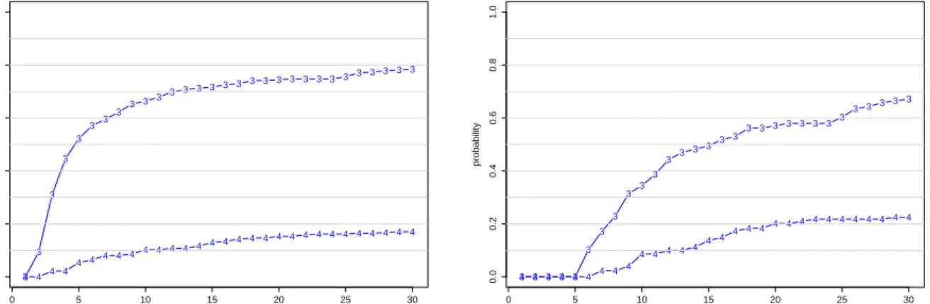
As mentioned above, patients can be discharged from the ICU to another ward or die inside the ICU. The time-dependent probabilities of these two terminal events were estimated using the approach described in Section 2.4 and are depicted in Figure 3 for s= 0 and for s = 5, with confidence intervals provided in Web Appendix D. The probability of being discharged alive from the ICU in the few first days is quite large (left panel of Figure 3). This corresponds to patients who were stabilized quickly and transferred to regular wards. The right panel of the figure shows that the corresponding cumulative incidence function increases much slower for those who stay five days in state 1. Figure 3 suggests that the probability to be discharged alive from the ICU is smaller for patients who are still in state 1 after five days compared to those who have just admitted to the ICU.
[Figure 3 about here.]
5. Discussion, main conclusions and final remarks
In this paper, two different nonparametric estimators of a transition probability matrix for a general progressive multi-state model have been investigated. Left-truncation and right-censoring issues which arise under cross-sectional sampling have been considered. The estimator based on product-limit integrals is consistent and shows the best performance in simulations when there is no censoring. With censored data, its consistency is not guaranteed whenever the censoring support is strictly contained in the lifetime support and, therefore, the alternative estimator is recommended. This alternative estimator follows ideas previously exploited in the right-censored setup (de U˜na- ´Alvarez and Meira-Machado, 2015; Titman, 2015). Even when other nonparametric approaches for left-truncated data exist, see e.g.
Titman (2015) and references therein, they ignore the individual trajectory before cross-section and, therefore, they are expected to be less efficient. We have illustrated this by comparing our methods to the Aalen-Johansen estimator which, despite of exploiting the Markov assumption, does not improve the new approach.
Other nonparametric methods to estimate the transition probability matrix have been proposed under the extra assumption of independence between the truncation time L and the residual censoring time C−L. Also, improved estimation may be obtained by including information (if available) on the distribution of the truncation time. With cross-sectional data, for example, some literature has been focused on the length-bias model in which the truncation variable is uniformly distributed. See Vakulenko-Lagun et al. (2017) for these alternative approaches. The two estimators considered in this paper are robust to these assumptions and are suitable when nothing is assumed on the distribution of L.
The estimators we study require complete information on transitions occurring before the truncation time. For applications involving medical records, obtaining the full history is often possible, as medical records are today computerized and quite detailed and reliable. However, there are situations in which the history is available only partially or not at all. Such cases can be dealt with under the Markov assumption using the Aalen-Johansen estimator and, for non-Markov processes, using the general approach described by Titman (2015).
Estimating regression effects on the transition probabilities may be conducted using pseu-dovalues (Klein and Andersen, 2005), obtained by one of the non-parametric estimators de-veloped in this paper. Alternatively, a direct binomial regression can be fitted, which requires the construction of suitable random weights for the indicator I(Z0,j 6t < T0,j). Azarang et al. (2017) dealt with this issue in the setting of the possibly non-Markov progressive illness-death model. With cross-sectional data, modified weights which take the left-truncation times into account are needed. Regression models may be restricted to covariates which are not
time-dependent, as retrospective information for the latter is rarely available. The details for the regression setting are currently under investigation, and will be presented elsewhere.
6. Supplementary Materials
Web Appendices A-D, referenced in Sections 2.2, 2.3, 2.6, 3, and 4 are available with this paper at the Biometrics website on Wiley Online Library.
Acknowledgements
The work was supported by Grant MTM2014-55966-P of the Spanish Ministerio de Econom´ıa y Competitividad and by The Israel Science Foundation (Grant No. 519/14).
References
Aalen, O., and Johansen, S. (1978). An empirical transition matrix for nonhomogeneous Markov chains based on censored observations. Scandinavian Journal of Statistics 5, 141–150.
Allignol, A., Beyersmann, J., Gerds, T., and Latouche, A. (2014). A competing risks approach for nonparametric estimation of transition probabilities in a non-Markov illness-death model. Lifetime Data Analysis 20, 495-513.
Andersen, P. K., Borgan, O., Gill, R. D., and Keiding, N. (1993). Statistical Models based on Counting Processes, Springer, New York.
Azarang, L., Scheike, T. and de U˜na- ´Alvarez, J. (2017). Direct modeling of regression effects for transition probabilities in the progressive illness–death model. Statistics in Medicine 36, 1964–1976.
Balboa, V., de U˜na- ´Alvarez, J. (2017). Estimation of Transition Probabilities for the Illness-Death Model: Package TP.idm. Journal of Statistical Software, in press.
distri-butions for truncated serial event data - a weighted-adjusted approach. Lifetime Data Analysis 12, 53–67.
Datta, S., and Satten, G. A. (2001). Validity of the Aalen-Johansen estimators of stage occupancy probabilities and Nelson Aalen estimators of integrated transition hazards for non- Markov models. Statistics & Probability Letters 55, 403-411.
de U˜na- ´Alvarez, J. (2017) Nonparametric estimation of an event-free survival distribution under cross-sectional sampling. In: From Statistics to Mathematical Finance Festscrhift in honor of Winfried Stute (Ferger, D., Gonz´alez-Manteiga, W., Schmidt, T., and Wang, J. L. Eds. ). Springer, 55–67.
de U˜na- ´Alvarez, J., and Meira-Machado, L. (2015). Nonparametric estimation of transition probabilities in the non-Markov illness-death model: a comparative study. Biometrics 61, 364–375.
de U˜na- ´Alvarez, J., and Veraverbeke, N. (2017). Copula-graphic estimation with left-truncated and right-censored data. Statistics 51, 387–403.
de Wreede, L. C., Fiocco, M., Putter, H. (2011). mstate: An R Package for the Analysis of Competing Risks and Multi-State Models. Journal of Statistical Software 38, 1–30. Hougaard, P. (2000). Analysis of Multivariate Survival Data, Springer, New York.
Klein, J. P. and Andersen, P. K. (2005) Regression modeling of competing risks data based on pseudo values of the cumulative incidence function. Biometrics 61, 223–229.
Mandel, M. (2010). The competing risks illness-death model under cross-sectional sampling.
Biostatistics 11, 209–303.
Meira-Machado, L. F., de U˜na- ´Alvarez, J., and Cadarso-Su´arez, C. (2006). Nonparametric estimation of transition probabilities in a non-Markov illness-death model.Lifetime Data Analysis 12, 325-344.
Journal of the American Statistical Association 86, 770-778.
Putter, H. and Spitoni, C. (2016). Non-parametric estimation of transition probabilities in non-Markov multi-state models: The landmark Aalen-Johansen estimator. Statistical Methods in Medical Research, published online.
S´anchez-Sellero, C., Gonz´alez-Manteiga, W., and Van Keilegom, I. (2005). Uniform repre-sentation of product-limit integrals with applications.Scandinavian Journal of Statistics 32, 563–581.
Stute, W. (1995). The central limit under random censorship. Annals of Statistics 23, 422– 439.
Stute, W., and Wang, J. L. (2008). The central limit theorem under random truncation.
Bernoulli 14, 604–622.
Titman, A. C. (2015). Transition probability estimates for non-Markov multi-state models.
Biometrics 71, 1034-1041.
Tsai, W.-Y., Jewell, N. P., and Wang, M.-C. (1987). A note on the product-limit estimator under right censoring and left truncation. Biometrika 74, 883–886.
Vakulenko-Lagun, B., and Mandel, M. (2016). Comparing estimation approaches for the illness–death model under left truncation and right censoring. Statistics in Medicine 35, 1533–1548.
Vakulenko-Lagun, B., Mandel, M., and Goldberg, Y. (2017). Nonparametric estimation in the illness-death model using prevalent data. Lifetime Data Analysis 23, 25–56.
van Houwelingen, H., Putter, H. (2012). Dynamic Prediction in Clinical Survival Analysis. Chapman & Hall / CRC, Boca Raton.
Zhou, Y., and Yip, P. S. F. (1999). A strong representation of the product-limit estimator for left truncated and right censored data. Journal of Multivariate Analysis 69, 261–280.
0 5 10 15 20 25 30 0 5 10 15 20 25 30 Truncation time T otal lif etime
Figure 1. Truncation times versus observed hospitalization times with the corresponding terminal observed states: blue crosses for death, circles for discharged alive, and red pluses for censoring. Patients who acquired BSIs are represented as vertical lines from BSI time (diamonds) to total observed time. This figure appears in color in the electronic version of this article.
0 5 10 15 20 25 30 0.0 0.2 0.4 0.6 0.8 1.0 time probability 0 5 10 15 20 25 30 0.0 0.2 0.4 0.6 0.8 1.0 time probability
Figure 2. Estimates of transition probabilities. Left - starting at s = 0, right - starting at s = 5. Black circles - product-limit type estimates and blue diamonds the alternative estimates. The curves at the top correspond to estimates of p11(s, t) while those at the
bottom, connected with lines, correspond to p12(s, t). This figure appears in color in the
4 4 4 4 4 4 4 4 4 4 4 4 4 4 4 4 4 4 4 4 4 4 4 4 44 4 4 4 4 0 5 10 15 20 25 30 0.0 0.2 0.4 0.6 0.8 1.0 time probability 3 3 3 3 3 33 33 3 33 3 3 3 3 33 3 3 3 3 3 3 3 3 3 3 3 3 4 4 4 4 4 4 4 4 4 4 4 4 4 4 4 4 4 4 44 4 4 4 4 4 4 4 4 4 4 0 5 10 15 20 25 30 0.0 0.2 0.4 0.6 0.8 1.0 time probability 3 3 3 3 3 3 3 3 33 3 33 3 3 3 3 3 3 3 3 3 3 3 3 3 3 3 3 3
Figure 3. Estimates of absorption probabilities. Left - starting at s = 0, right - starting at s= 5. The numbers indicates the absorbing state (3-discharged alive, 4-died in the ICU)
p11(s,1) p12(s,1)
s method n bias×103 MSE×103 quantile bias×103 MSE×103 quantile
0 pl 100 0.673 0.426 93.5% 9.964 8.807 92.0% 0 new 100 1.926 0.675 93.5% 8.711 8.945 93.2% 0 pl 200 0.862 0.246 92.5% 1.066 4.750 94.0% 0 new 200 1.755 0.349 94.2% 0.162 4.804 94.8% 0 pl 500 0.190 0.085 95.2% 1.596 2.274 92.0% 0 new 500 0.199 0.117 95.0% 1.587 2.342 92.5% 0 pl 1000 0.264 0.044 94.2% 1.401 1.065 93.2% 0 new 1000 0.098 0.053 95.8% 1.566 1.087 93.0% 0.1 pl 100 -0.585 0.654 93.8% 0.126 7.701 94.0% 0.1 new 100 -0.612 0.954 92.0% 0.153 8.036 93.0% 0.1 pl 200 -0.707 0.269 96.8% -1.724 3.466 94.5% 0.1 new 200 -1.470 0.458 93.2% -0.960 3.676 94.0% 0.1 pl 500 0.071 0.120 96.2% 1.268 1.436 95.2% 0.1 new 500 -0.658 0.187 94.8% 1.998 1.478 95.5% 0.1 pl 1000 -0.974 0.062 95.8% -2.657 0.769 94.0% 0.1 new 1000 -1.260 0.096Table 194.5% -2.374 0.782 93.5%
Simulation results for the uncensored case based on 400 replications. The transition probabilities are from timesto time1, and the true values arep11(0,1) = 0.050,p12(0,1) = 0.455, p11(0.1,1) = 0.067,p12(0.1,1) = 0.464. Methods
pl and new are the product-limit and the alternative estimators, respectively; quantile is the empirical coverage of the 95% confidence interval.
p11(s,1) p12(s,1)
s method n bias×103 MSE×103 quantile bias×103 MSE×103 quantile
0 pl 100 34.894 4.284 88.2% -37.993 9.714 90.5% 0 new 100 -0.552 0.529 90.5% -2.547 6.744 93.2% 0 pl 200 24.092 1.861 88.2% -19.325 4.342 93.2% 0 new 200 0.687 0.234 94.8% 4.080 3.018 93.8% 0 pl 500 12.174 0.608 90.5% -9.771 1.692 93.8% 0 new 500 0.313 0.116 92.8% 2.090 1.282 94.2% 0 pl 1000 7.186 0.284 91.5% -8.104 1.031 94.0% 0 new 1000 -0.128 0.044 95.2% -0.789 0.833 94.5% 0.1 pl 100 32.889 5.180 90.2% -30.360 9.190 89.8% 0.1 new 100 -0.322 0.828 92.8% 2.851 5.323 92.0% 0.1 pl 200 24.143 2.493 91.2% -24.112 4.328 91.2% 0.1 new 200 1.715 0.419 91.5% -1.684 2.574 93.5% 0.1 pl 500 9.764 0.679 93.2% -11.146 1.516 93.0% 0.1 new 500 -0.881 0.165 93.2% -0.502 1.076 93.0% 0.1 pl 1000 9.007 0.374 92.8% -8.165 0.846 91.0% 0.1 new 1000 0.372 0.080Table 294.8% 0.468 0.539 94.8%
Simulation results for the fixed follow-up case based on 400 replications. The transition probabilities are from times
to time1, and the true values arep11(0,1) = 0.050, p12(0,1) = 0.455,p11(0.1,1) = 0.067,p12(0.1,1) = 0.464.
Methods pl and new are the product-limit and the alternative estimators, respectively; quantile is the empirical coverage of the 95% confidence interval.
p11(s,1) p12(s,1)
s method n bias×103 MSE×103 quantile bias×103 MSE×103 quantile
0 pl 100 77.886 7.292 23.5% -69.696 11.304 85.2% 0 new 100 0.829 0.623 93.5% 7.361 8.784 92.5% 0 pl 200 77.469 6.699 8.5% -66.951 7.728 80.5% 0 new 200 -0.255 0.281 93.5% 10.760 4.795 93.2% 0 pl 500 78.805 6.504 2.2% -75.981 7.263 41.8% 0 new 500 0.719 0.120 95.0% 2.105 2.106 94.8% 0 pl 1000 77.703 6.199 1.5% -74.329 6.436 16.8% 0 new 1000 0.618 0.059 94.8% 2.756 1.351 90.8% 0.1 pl 100 69.345 6.384 51.8% -76.022 12.152 83.2% 0.1 new 100 -0.167 0.974 91.0% -6.511 8.457 94.0% 0.1 pl 200 70.440 5.600 12.2% -70.394 7.636 74.5% 0.1 new 200 -0.525 0.509 92.0% 0.571 3.340 95.0% 0.1 pl 500 69.722 5.158 0.0% -71.445 6.321 44.2% 0.1 new 500 -0.587 0.201 94.0% -1.137 1.486 96.2% 0.1 pl 1000 68.996 4.905 0.0% -72.769 5.942 15.0% 0.1 new 1000 -0.543 0.083Table 397.0% -3.234 0.839 93.5%
Simulation results for the fixed censoring time case based on 400 replications. The transition probabilities are from times to time1, and the true values arep11(0,1) = 0.050,p12(0,1) = 0.455,p11(0.1,1) = 0.067, p12(0.1,1) = 0.464.
Methods pl and new are the product-limit and the alternative estimators, respectively; quantile is the empirical coverage of the 95% confidence interval.
s t C model pl11 pl12 new11 new12 AJ11 AJ12 0 1 C =∞ 0.20 3.80 0.29 3.84 0.55 5.12 0.5 1 C =∞ 3.01 5.04 4.17 6.24 5.13 4.99 0 1 C =L+ 0.5 14.34 15.16 0.53 4.65 0.74 4.94 0.5 1 C =L+ 0.5 30.11 30.69 7.52 10.77 8.66 8.41 0 1 C ∼U(0,2.5) 14.28 15.23 0.34 3.58 0.51 4.05 0.5 1 C ∼U(0,2.5) 26.23 Table 427.59 4.41 6.97 5.03 5.18
MSE×103 under a Markov illness-death model based on 1000 replications each with sample size n= 200. pl - the product-limit type estimator, new - the alternative estimator, AJ - the Aalen-Johansen estimator. Labels 11 and 12