Distortionary Taxation for
Efficient Redistribution
Borys Grochulski
T
his article uses a simple model to review the economic theory of efficient redistributive taxation. Three main results are presented. The first is the classic competitive equilibrium efficiency result: trade in competitive markets leads to an efficient final (i.e., equilibrium) allocation of consumption among the agents in the economy. The equilibrium allocation is determined by market supply and demand forces. In our model economy, the equilibrium allocation is determined uniquely. This efficiency result, known as the First Welfare Theorem, provides a strong argument supporting the view that unobstructed competitive market forces can be relied on to determine the allocation of consumption in the economy. One must observe, however, that the competitive market equilibrium supports one efficient allocation, i.e., competitive markets support one particular distribution of the total gains from trade that are available in the economy. There are an infinite number of ways in which the total gains from trade can be efficiently divided among the agents. Thus, absent redistribution, almost all efficient divisions of the gains from trade areinconsistentwith the competitive market mechanism. In other words, the competitive market mechanism guarantees efficiency but also imposes on the society one particular division of the welfare gains from trade. It is entirely possible that the agents in the economy may prefer to divide the gains from trade differently. In fact, there is no a priori reason to believe that the society’s most preferred division of the gains from trade should happen to coincide with that imposed by the market mechanism. Thus, for distributional reasons, the competitive market allocation will almost surely be suboptimal.The second result we review describes the classic solution to the distribu-tional problems associated with the competitive market mechanism: wealth
The author would like to thank Kartik Athreya, Leonardo Martinez, Sam Henly, and Ned Prescott for their helpful comments. The views expressed in this article are those of the author and do not necessarily reflect those of the Federal Reserve Bank of Richmond or the Federal Reserve System. E-mail: [email protected].
transfers. If society prefers a different division of the gains from trade than the one brought about by competitive market forces, it is sufficient to transfer wealth among the agents in order to correct it. Such wealth transfers can be implemented via simple lump-sum transfers and taxes levied by the gov-ernment. This result, known as the Second Welfare Theorem, however, poses strong requirements on the quality of information available to the government. Lump-sum taxes, by definition, depend only on agents’ types (and not on their actions). In order to use lump-sum taxes, thus, the government must possess sufficient information about agents’ types, on a person-by-person basis. If public information is not sufficiently detailed, the required wealth transfers and taxes cannot be applied because the government is unable to determine which agents should be taxed and which should receive a transfer. In this situation, the Second Welfare Theorem breaks down: Lump-sum taxes are insufficient to achieve any division of the gains from trade other than the one implied by the competitive market mechanism.
The third result we review concerns the problem of efficient redistribution of the total gains from trade in the case of incomplete public information. Here, the inefficacy of lump-sum taxes creates a role for distortionary taxa-tion. A tax is called distortionary if the amount due from an agent depends on his actions. If an activity is subject to a distortionary tax, then by avoiding the activity the agent can avoid the tax, which distorts his incentive to engage in this activity. The ability to influence agents’ incentives is exactly what makes distortionary taxes useful. The tax-imposed distortions can be designed to offset the distortions resulting from incomplete information. Such corrective distortions, clearly, cannot be generated by lump-sum taxes, which are nondis-tortionary. The third main result we review in this article is a version of the Second Welfare Theorem modified to include distortionary taxes. Within our model economy, we fully characterize a distortionary tax system sufficient to achieve any efficient division of the gains from trade available in our economy when public information is incomplete. This tax system consists of a lump-sum-funded subsidy to sufficiently large capital trades. Depending on which among the infinite number of efficient divisions of the gains from trade is to be implemented, the subsidy can go to either those who sell or to those who buy capital in the competitive market.
The model economy is a two-period, deterministic Lucas-tree economy in which income comes from a stock of productive capital. In each period, one unit of the capital stock producesy units of a single, perishable consumption good. The capital stock is fixed, i.e., no physical investment is possible. The size of the economy’s total capital stock is normalized to unity. Agents, who own the capital stock in equal shares, are heterogenous with respect to their preference for early versus late consumption. In particular, there are two types of agents in this economy: the patient ones, whose marginal utility from
consuming in the first period is relatively low, and the impatient ones, whose marginal utility from consuming in the first period is relatively high.
Efficient divisions of the welfare gains from trade are represented by Pareto-efficient allocations of consumption. For the model economy we consider, Pareto-efficient allocations of consumption are characterized in Grochulski (2008). This characterization describes the full set of possibil-ities for feasible and efficient division of the total gains from trade among the patient and impatient agents—both in the case of complete public information and in the case of agents’ private knowledge of their impatience type. Having this description in hand, we can consider, in the present article, the question of how any given such division can be implemented in a competitive market economy. In particular, we focus on the role the government has in supporting the socially preferred division of total gains from trade through redistributive taxation.
The question of efficient redistribution and its implementation through taxation has long been studied in economics. The definitive treatment of the classical theory of efficiency and distributional properties of competitive markets under full information and with no externalities is given in Debreu (1959).1 The first two of the three main results we review in this article are
simple special cases of the welfare theorems provided in Debreu (1959).2 In
a seminal paper, Mirrlees (1971) takes on the same question while explicitly recognizing that government information may be incomplete. The third main result we present is a version of the optimal distortionary taxation result of Mirrlees (1971). Our model economy differs from that of Mirrlees (1971) in that ours is a pure-capital-income, general equilibrium economy while in the one studied in Mirrlees (1971) all income comes from labor. Mathematically, however, our model economy is a simplified version of the model studied in Mirrlees (1971).
Stiglitz (1987) reviews the literature on optimal redistributive taxation in economies with private information.3 Kocherlakota (2007) surveys a related literature on tax systems implementing optimal social insurance in dynamic economies with ex-post private information.
The body of this article is organized as follows. Section 1 describes in detail the economy we study. Section 2 defines competitive equilibrium. Section 3 demonstrates the efficiency of competitive equilibrium indirectly as well as through direct computation. Section 4 shows the sufficiency of lump-sum taxes for efficient redistribution under full information. Also, it
1 Pigou (1932) initiated the by now extensive, and still actively developing, literature on corrective distortionary taxation in economies with externalities.
2 Chapter 16 of Mas-Colell, Whinston, and Green (1995) contains an excellent textbook treat-ment of these results.
demonstrates the inefficacy of lump-sum taxes when agents’ types are not ob-served by the government. Section 5 defines a general class of distortionary tax systems. There, also, it is shown that a simple tax system with a pro-portional distortionary tax on capital income is incapable of providing any redistribution. Section 6 is devoted to the study of an optimal distortionary tax system in which capital taxes are nonlinear. Section 7 discusses alternative optimal tax systems. Section 8 concludes.
1. A SIMPLE PURE CAPITAL INCOME ECONOMY
In this article, we will study a private-ownership version of the economic environment also studied in a companion article, Grochulski (2008, referenced hereafter as G08 for short). The economy is populated by a unit mass of agents who live for two periods,t =1,2. There is a single consumption good each period,ct, and agents’ preferences over consumption pairs (c1, c2)are represented by the utility function
θ u(c1)+βu(c2), (1)
whereβ is a common-to-all discount factor, andθ is an agent-specific pref-erence parameter. Agents are heterogenous in their relative prefpref-erence for consumption at date 1. We assume a two-point support for the population distribution of the impatience parameter, θ. Agents, therefore, are of two types. A fraction,μH, of the agents are impatient with a strong preference for consuming in period 1. Denote byHthe value of the preference parameter,θ, that represents preferences of the impatient agents. A fraction,μL=1−μH, are agents of the patient type. Their value of the impatience parameter, θ, denoted byL, satisfiesL < H.
The production side of the economy is represented by the so-called Lucas tree. Each agent is endowed with one unit of productive capital stock—the tree. Each period, one unit of the capital stock producesyunits of the consumption good—the fruit of the tree. Given that the total mass of agents is normalized to unity and each agent is endowed with one tree, the aggregate amount of the consumption good available in this economy in each of the two periods is
Y =y. The consumption good is perishable—it cannot be stored from period 1 to 2. The size of the capital stock, i.e., the number of trees, is fixed: Capital does not depreciate nor can it be accumulated.
Note that there is no uncertainty in this economy. In particular, agents’ impatience parameter,θ, is nonstochastic. The production side of the economy is deterministic as well.
For simplicity and clarity of exposition, as in G08, we will focus our atten-tion on a particular set of values for the preference and technology parameters.
In particular, we take u(·)=log(·), β = 1 2, H = 5 2, L= 1 2, μH =μL= 1 2, y =1. (2) Roughly, the model period is thought of as being 25 years. The value of the discount factor,β, of 12 corresponds to an annualized discount factor of about 0.973. The fractions of the two patience types are equal; preferences are logarithmic. The per-period product of the capital stock,y=Y, is normalized to 1.
An allocation in this economy is a description of how the total output (i.e., the total capital income,Y) is distributed among the agents each period. An allocation, therefore, is given byc=(c1H, c1L, c2H, c2L), wherect θ ≥0 denotes the amount of the consumption good in periodtassigned to each agent of typeθ. To be resource-feasible, allocations must satisfy
θ=H,L
μθct θ ≤Y, (3)
fort = 1,2, i.e., the aggregate consumption must not exceed the aggregate output.4 Given the utility functions (1), an allocation, c, gives total utility
(or welfare),θ u(c1θ)+βu(c2θ), to each agent of type θ = H, L. For any
α∈[0,1], the social welfare function is a weighted average of the utilities of the two types of agents:
α[H u(c1H)+βu(c2H)]+(1−α)[Lu(c1L)+βu(c2L)], (4) where α represents the absolute weight the society attaches to the welfare of the agents of typeH. Let γ = α/(1−α)denote the relative weight of the agents of typeH. An allocation is Pareto efficient if there does not exist a feasible re-allocation that some agents would desire and no agents would oppose. In this sense, Pareto-efficient allocations represent all divisions of the total gains from trade that can be attained in the economy.
As discussed in G08, one can find all Pareto-efficient allocations by solv-ing, for eachγ ∈[0,+∞], the problem of maximization of the social welfare function (4) subject to feasibility constraints. If all information in the econ-omy is public, these feasibility constraints are simply the resource feasibility constraints (3). The allocation,c, attaining the maximum of the social welfare function (4) for a given value of the relative weight,γ, is called a First Best Pareto optimum, and is denoted byc∗(γ ). By adjustingγ between 0 and+∞, we can trace out the set of all First Best Pareto optima in this economy. This set is depicted in Figure 1 of G08.
The assumption of complete public information may be too strong. In particular, the government may be unable to observe agents’ preferences. For
4 Note that this constraint is independent of how the aggregate output is initially allocated to the agents.
this reason, we will consider the assumption that each agent’s impatience pa-rameter, θ, is known only to the agent himself and not to anybody else in the economy. This incompleteness of public information imposes additional restrictions on the feasible re-allocations that can be implemented in the econ-omy. As discussed in G08, these restrictions take the form of the so-called incentive compatibility constraints, which are given by
H u(c1H)+βu(c2H)≥H u(c1L)+βu(c2L)and (5)
Lu(c1L)+βu(c2L)≥Lu(c1H)+βu(c2H). (6) Suppose the government presents the agents with an allocation,c, and asks them to reveal their impatience parameter. Ifcsatisfies these constraints, the agents will have no incentive to misrepresent their true type.
In the economy with private information, all Pareto-efficient allocations can be found by maximizing, again for eachγ ∈[0,+∞], the social welfare function (4) subject to resource feasibility constraints (3) and the incentive compatibility constraints (5) and (6). The allocation,c, attaining the maximum in this problem for a given value ofγ is denoted byc∗∗(γ )and often called a constrained-Pareto or Second Best Pareto optimum. This name reflects the fact thatc∗∗(γ ) is efficient in a more narrow sense than the corresponding
c∗(γ ), asc∗∗(γ )is constrained by private information whilec∗(γ )is not. The set of all Second Best Pareto optima for this economy is depicted in Figure 4 of G08.
G08 provides a fairly detailed characterization of the sets of First and Second Best Pareto-optimal allocations. In the present article, we will exam-ine the relation between Pareto-optimal allocations and market equilibrium allocations. We begin by describing the competitive market mechanism and its equilibrium.
2. COMPETITIVE CAPITAL MARKET EQUILIBRIUM
In this article, we study a private-ownership economy in which all agents are initially endowed with one unit of productive capital. Relative to this initial allocation, clearly, there are gains from trade to be exploited (i.e., the initial allocation is not a Pareto optimum). When income generated by the capital stock (i.e., the dividend) is realized in the first period, all agents have the same amount of the consumption good in hand (y units), and the same amount of consumption they will receive in the next period (y units again), but not the same desire to consume now versus next period. Thus, it is natural for them to trade consumption in hand today for capital, i.e., for the dividends, that will be received tomorrow. The relatively impatient agents, i.e., those whose preference type isθ = H, can sell some of their capital to the more patient agents of typeθ =Lin return for current consumption. This can be done for the mutual benefit of the two types of agents because their preferences differ.
The terms of this mutually beneficial trade, which will determine the final division of the welfare gains from trade, can depend on many factors. How many units of consumption in the first period will a patient agent be willing to pay for a unit of capital being sold by the impatient agent? Given the economic environment, a reasonable answer to this question is: the market price. In this environment, we have a large number of sellers of capital (massmH to be exact) and a large number of buyers (mass mL). Also, we do not assume that buyers or sellers face any technological barriers to trading like significant costs of shopping around, communicating, or negotiating with potential trade counterparties. Therefore, no rational agent will trade with a counterparty unless he is confident that he cannot obtain more favorable terms of trade by continuing to shop around. The competitive market price of capital represents the terms of trade that give this confidence to a rational agent. It is reasonable to expect that a competitive market for capital will emerge in this environment. Let us therefore consider the standard formal model of the competitive market mechanism. After agents collect dividends in period 1, they choose the quantity,c1, that they consume now, the quantity,a, of capital they purchase or sell at the market price, q, and the quantity they will be consuming in the second period, c2. Their initial endowment of capital and its price, q, determine the set of consumption pairs(c1, c2)that are affordable.
Formally, agents of typeθ =H, Lchoosec1,a, andc2so as to solve the following individual utility maximization problem:
max c1≥0,c2≥0,a
θ u(c1)+βu(c2),
subject to the budget constraints
c1+qa ≤ y, (7)
c2 ≤ (1+a)y. (8)
Note that the non-negativity requirement for consumption at the second date implies thata ≥ −1, i.e., no agent can sell more capital than the one unit he owns.
LetcD
t θ(q)fort =1,2 andaDθ (q)forθ =H, Ldenote the agents’ demand functions for consumption and capital, respectively, i.e., the solutions to the above individual optimization problem for any given price of capital,q. Definition 1 Competitive market equilibrium consists of a consumption allo-cation,cˆ =(c1ˆ H,c1ˆ L,c2ˆ H,c2ˆ L); capital trades,aˆ =(aˆH,aˆL); and a capital price,qˆ, such that
(i) agents optimize, i.e., the equilibrium allocation maximizes agents’ utility given the equilibrium price,qˆ:
ˆ
ct θ = ct θD(q),ˆ
ˆ
aθ = aθD(q),ˆ fort=1,2andθ =H, L;
(ii) the capital market clears:
θ=H,L
μθaˆθ =0. (9)
Note that the budget constraints and the capital market clearing condition imply that the equilibrium allocation of consumption is resource-feasible, i.e., the sum of all agents’ consumption in every period does not exceed the total amount of output,Y:
θ=H,L
μθcˆt θ ≤Y (10)
fort=1,2.
3. EFFICIENCY OF CAPITAL MARKET EQUILIBRIUM
Suppose there is no government intervention and agents trade freely. As a result, each agent obtains some final allocation of consumption. As we discussed in the previous section, we expect this allocation to be a competitive equilibrium allocation, cˆ. The following is the classic competitive market optimality result.
Theorem 1 Let(c,ˆ a,ˆ q)ˆ be a competitive capital market equilibrium. Then, the equilibrium allocation of consumption,cˆ, is Pareto optimal.
Recall that an allocation is Pareto optimal (or Pareto efficient) if it is feasible and not Pareto dominated by another feasible allocation. An allocation
xPareto dominates an allocationzif all agents in the economy preferxover
z, and at least one agent in the economy prefersx overz strictly.5 Clearly,
a Pareto-dominated allocation is a waste. If all agents can be made better off including at least one agent strictly, it would be a waste to not exploit this opportunity. The above theorem tells us that competitive equilibrium allocation is free of this failure. This important result, which holds much more generally than just in our simple capital market model, is often called the First Welfare Theorem.
A General Proof of the First Welfare Theorem
In this subsection, let us present a general, standard argument behind the First Welfare Theorem.6 We will note that this argument is an indirect one.
5 G08 provides additional discussion of Pareto dominance and feasibility with full and partial public information.
6 See also Mas-Colell, Whinston, and Green (1995) for an excellent textbook treatment of this result.
We begin with the following simple implication of agents’ utility maxi-mization: In equilibrium, it must be the case that
ˆ
c1θ + ˆc2θq/yˆ =y+ ˆq. (11) To see this, note first that when agents optimize, their budget constraints will be satisfied as equalities because utility is strictly increasing in consumption. Then, eliminateaˆθ from (7) and (8) to obtain (11).
Equation (11) represents the fact that in equilibrium agents will not waste personal wealth. The right-hand side of (11) represents the equilibrium value of each agent’s initial endowment of capital in terms of the units of first-period consumption. In first-period 1, an agent can collect dividendy and then sell all his capital endowment forqˆ. Thus, his total wealth is y+ ˆq. The left-hand side of (11) represents the cost of the consumption allocation, cˆθ. In equilibrium, qyˆ is the price of one unit ofc2in terms of the units ofc1: It takes y1 units of capital to obtain one unit of consumption in period 2, andq
units of consumption in period 1 to obtain one unit of capital. Effectively, it takes qyˆ units of consumptionc1to obtain one unit of consumptionc2. Thus,
ˆ
c1θ+ ˆc2θq/yˆ is the cost of the consumption paircˆθ =(c1ˆ θ,c2ˆ θ).
Now suppose that a feasible allocationc¯Pareto dominates the equilibrium allocationcˆ. This means that agents of at least one type strictly preferc¯θover
ˆ
cθ, and both types preferc¯θ overcˆθ at least weakly. Because utility is strictly increasing in consumption,c¯θ must be strictly unaffordable to all those who strictly prefer it and at best just affordable to those who weakly prefer it (which is everybody).7 Thus, for bothθ,
¯
c1θ+ ¯c2θq/yˆ ≥ ˆy+q (12) with at least one of these two inequalities being strict. Multiplying this in-equality for typeθ byμθand adding overθ, we obtain
θ=H,L μθc1¯ θ + θ=H,L μθc2¯ θ ˆ q/y > θ=H,L μθ(y+ ˆq),
where the inequality is strict because at least one of the inequalities in (12) is strict. Sincec¯is feasible, it must satisfy the resource constraints (10). Using these, we obtain from the above that
Y +Yq/y > yˆ + ˆq.
7 Note that this argument relies only on the strict monotonicity of preferences (and, in fact, could rely only on local nonsatiation; see Mas-Collel, Whinston, and Green [1995], section 16 C). In our model, we could actually make a stronger argument based on the strict convexity of preferences. Namely, since agents’ preferences are strictly increasing and strictly convex, cˆθ is a unique maximizer of utility in the budget set. Thus, c¯θ must be strictly unaffordable even to the type that is indifferent between cˆθ and c¯θ.
SubstitutingY =ywe get
Y + ˆq > Y + ˆq,
which is a contradiction. Thus, a feasible allocation,c¯, that Pareto dominates the equilibrium allocation,cˆ, cannot exist.
A Direct Proof of the First Welfare Theorem
The First Welfare Theorem tells us that any equilibrium allocation is Pareto optimal and nothing more. In particular, the general, indirect proof of the First Welfare Theorem tells us nothing about which among the infinitely many Pareto-optimal allocations the equilibrium allocationcˆcoincides with. This question, which strictly speaking is outside the scope of the First Welfare Theorem, may be of independent interest.
In the specific environment that we consider in this article, we can give a direct proof of the First Welfare Theorem. Namely, we can compute the set of competitive equilibrium allocations and compare it against the set of all Pareto-optimal allocations. In this way, we will be able to tell exactly which Pareto optima can be implemented as competitive equilibria.
Solving the individual utility maximization problem
We begin by deriving the agents’ capital demand functions. Similar to (11), we can rewrite the agents’ budget constraints as an equality of the present value of consumption and wealth:
c1+c2q/y =y+q. (13)
In this form, it is easy to see the agents’ utility maximization problem has a linear budget set and a strictly concave objective function. Thus, at each price,
q, it has a unique solution, which we can compute from the budget constraint (13) and the Euler equation8
θ u(c1)q/y=βu(c2). (14)
For each θ, we solve these two equations to obtain consumption demand functionscD
t θ(q)fort =1,2. Using the parameter values in (1), these solutions are cD1θ(q) = 2θ 1+q 1+2θ, cD2θ(q) = 1 q 1+q 1+2θ.
8 Perhaps the simplest way to obtain the Euler equation (14) is to express the utility maxi-mization problem as maxc2θ u(y+q−c2q/y)+βu(c2) and take the first-order condition.
From (8) evaluated at equality, we obtain that typeθ’s capital demand function is aθD(q)= 1 q 1+q 1+2θ −1.
Solving for equilibrium price of capital and allocation
Substituting the capital demand functions into the capital market clearing condition (9) and solving for the price that clears this market, we obtain an equilibrium priceqˆ = 12. It is easy to see that there are no other prices that clear this market, i.e., the competitive equilibrium is unique in our model.9
We can now compute equilibrium capital trades:
ˆ aL = aLD( 1 2)= 1 2, ˆ aH = aHD( 1 2)= − 1 2, and the equilibrium allocation of consumption:
ˆ cL = ˆ c1L,c2ˆ L = 3 4, 3 2 , (15) ˆ cH = ˆ c1H,c2ˆ H = 5 4, 1 2 . (16)
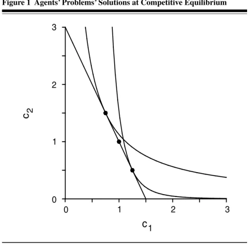
Figure 1 depicts the agents’ budget constraint at the equilibrium capital price,qˆ = 12; equilibrium consumption pairs (15) and (16); and one indiffer-ence curve for each type of agent. Clearly, both agent types face the same budget constraint. Since their preferences differ, so do their choices. The in-difference curve depicted for each typeθrepresents the highest level of utility that each type attains within the budget constraint. Note also that point (1,1) in Figure 1 represents the consumption bundle that agents get if they do not trade. In equilibrium, the impatient agent exchanges14 units ofc1for 12 units ofc2. The patient agent, of course, takes the opposite end of this trade. Confronting equilibrium with the set of Pareto-optimal
allocations
Our first observation here is that the competitive capital market mechanism delivers a unique equilibrium allocation of consumption. We observe next that, as shown in detail in G08, there is a continuum of Pareto-optimal allocations
9 Expressed as a function of gross return on capital investment,R= 1q, rather than the price of capital, q, agents’ demand for capital is linear in R. Namely, aDθ (R)= 1R++21θ −1. Thus, for any two numbers, θ, there can be at most one solution to the capital market clearing condition, so equilibrium is unique.
Figure 1 Agents’ Problems’ Solutions at Competitive Equilibrium
0
1
2
1
2
3
0
3
c
1
2c
in our environment.10 From these two observations, we immediately see
thatalmost allPareto-optimal allocations areincompatiblewith competitive equilibrium.
Which one among the continuum is the Pareto optimum consistent with competitive equilibrium? Formulas (8)–(11) in G08 describe the set of all First Best Pareto optima indexed by parameterγ ∈ [0,∞] representing the relative welfare weight assigned to the impatient agents in the social objective function. If society favors neither of the two types of agents, the welfare weight given to both types is the same, i.e., the relative weight of the impatient type,
γ, is 1. Thus, γ = 1 represents the so-called utilitarian Pareto optimum. ByγCElet us denote the value of the index,γ, associated with the optimum that is selected by the market mechanism in competitive equilibrium. From
10 Multiplicity of Pareto-optimal allocations is typical in environments with heterogenous agents.
formulas (8)–(11) in G08, we obtain immediately that the unique competitive allocation,cˆ, given in (15) and (16) is the Pareto optimum corresponding to
γ =1/3, i.e.,γCE =1/3 in our economy. Thus, competitive equilibrium is optimal if and only if society values welfare of the patient type,L, three times as much as it values welfare of the impatient type,H.
Why this Pareto Optimum?
As we have seen, competitive capital market equilibrium implements a rather particular Pareto optimum. Intuitively, we see that the competitive capital market selects a Pareto optimum that “favors” the patient agents. With a large mass of agents whose desire for consumption in the first period is very strong relative to the population average (Hexceeds the averageθby 66 percent), the market is “flooded” with capital, which becomes very affordable to the patient agents.11 As the impatient agents compete for first-period consumption, the
patient agents end up receiving two units ofc2for each unit ofc1in equilibrium. That rate of exchange is optimal only if society on the whole cares for the welfare of the patient agents more than it cares for the welfare of the impatient consumers.12
In conclusion, the competitive market mechanism does two things: it allows the agents to obtain welfare gains from trade, and it also divides these gains among the agents in a particular way. It is entirely possible that society might desire a different division of the welfare gains than the one built into the competitive market allocation mechanism. This problem creates a role for redistributive government policy. In the remainder of this article, we consider how the government can supplement the competitive market mechanism with a tax system that preserves efficiency but implements other divisions of the welfare gains from trade.
In the next section, we consider the situation in which the government has full information on each agent’s preference type and, therefore, can transfer wealth from one type to another as a lump sum. Subsequently, we consider
11 To see this point more clearly, note that the preferences of the patient type can be alter-natively represented by log(c1)+log(c2) and qˆ= 12.
12 As a simple thought experiment, consider the question of how the competitive equilibrium selection from the Pareto set changes when the relative impatience of the two types of agents changes. In particular, suppose that L is not necessarily 12 but can be any real number smaller or equal toH. Let γCE(L) denote the index of the Pareto optimum that is implemented by the competitive equilibrium as L is adjusted between 0 and 52. It is easy to show that γCE(L)= (2L+1)/6. Thus, competitive equilibrium selects the utilitarian Pareto optimum only if all agents are identical (no trade is optimal in this case). When the impatient agents become very impatient, i.e., when L approaches 0, we have that γCE(0)= 16, i.e., competitive equilibrium selects the Pareto optimum that would be selected by a society that values welfare of the patient typeL six times as much as it values welfare of the impatient type H.
private information, which makes lump-sum wealth transfers infeasible and creates a role for distortionary redistributive taxation.
4. COMPETITIVE EQUILIBRIUM WITH LUMP-SUM TAXES
We begin by extending the definition of competitive equilibrium (i.e., Defini-tion 1) to allow for lump-sum wealth transfers. A tax on an agent is lump-sum if the amount due is independent of any choices made by this agent. For ex-ample, a labor income tax is not lump-sum because the amount due increases with the number of hours the agent chooses to work. Taxes under which the amount due does depend on the taxpayers’ choices are called distortionary.
In our economy, agents choose consumption in periods 1 and 2 and their capital holdings in period 2. Thus, lump-sum taxes must not depend on con-sumption or capital holdings. Agents’ impatience typeθ, however, is not their choice. If the government can observe each agent’s typeθ, a lump-sum tax can depend onθ. In this section, we assume that each agent’s preference type
θ is freely and publicly observable. In particular, the government sees every agent’s type and therefore can impose different lump-sum taxes on the agents of different types.
In this setting, a lump-sum tax system consists of two real numbers: TH andTL, where a negative value ofTθ means a transfer from the government to the agent of typeθ. Under these taxes, the budget constraints of the agents of typeθ =H, Lare
c1+aq ≤ y−Tθ,
c2 ≤ (1+a)y,
whereq, as before, is the ex-dividend price of capital in the first period. Note that the lump-sum taxesTθare levied in period 1 and denominated in the units of consumption at that date. It is entirely possible to levy lump-sum taxes at both dates, but it is easy to see that doing this would not be useful. Treating the budget constraints as equalities, eliminatinga, we can express the budget constraint in the present value as follows:
c1+c2q/y =y+q−Tθ. (17)
From here we see that any lump-sum tax at the second date can be lumped intoTθ.
Competitive equilibrium with lump-sum taxes, (Tθ)θ=H,L, is defined analogously to the tax-free competitive equilibrium of Definition 1: A price-allocation pair will be an equilibrium if agents optimize, now subject to (17), and markets clear. In addition, the government must break even in equilibrium, i.e., taxes,(Tθ)θ=H,L, must satisfy the government budget constraint
θ=H,L
Efficient Redistribution with Lump-Sum Taxation Under Full Information
We will say that a lump-sum tax system,(Tθ)θ=H,L, implements a given allo-cation,c, ifcis a competitive equilibrium allocation under taxes,(Tθ)θ=H,L. The following result is a version of the classic sufficiency result known as the Second Welfare Theorem.
Theorem 2 Every First Best Pareto optimum,c∗, can be implemented with a lump-sum tax system,(Tθ)θ=H,L.
Under this theorem, lump-sum taxes are clearly sufficient to achieve any desired distribution of the total gains from trade available in this economy.
We will now provide a proof of this theorem constructed as follows. First, we derive a set of sufficient conditions for an allocation to be an equilibrium allocation. Then, we show that for every First Best Pareto optimumc∗(γ ),
γ ∈ [0,∞], lump-sum taxes, (Tθ)θ=H,L, can be set so c∗(γ )satisfies these sufficient conditions.
In order for an allocation,c, to be an equilibrium allocation, there must exist a capital price,q, at which agents choose to consumecand the capital trades associated with c clear the market. First, let us identify sufficient conditions for agents’optimization at a given price,q. Under the present-value budget constraint (17), agents solve a strictly concave optimization problem. Thus, the individual Euler equation (14) and the budget constraint (17) are sufficient for an allocation,c, to be individually optimal at the price,q. Second, we need to check market clearing. However, as long as we implement a resource-feasible allocation, c, the capital purchases associated withc will clear the market.
One of the properties of the First Best Pareto optima (FBPO) is that they are free of the so-calledintertemporal wedges(see G08, Section 3). This means that at each FBPOc∗(γ )the intertemporal marginal rate of substitution (IMRS) of each agent type is equal to the intertemporal marginal rate of transformation. Denote the IMRS of agent typeθ evaluated at a FBPO allocationc∗(γ )by
m∗θ(γ ), i.e.,
m∗θ(γ )= βu
(c∗
2θ(γ ))
θ u(c1∗θ(γ )). (19)
The lack of intertemporal wedges demonstrated in G08 implies that
m∗H(γ )=m∗L(γ )
for eachγ ∈ [0,∞]. This simple property is crucial for the implementation of FBPO as competitive equilibria.
Let us denote the two agent types’ common IMRS value by m∗(γ ). Directly from (14) we see that if the price of capital is
then the individual Euler equation holds for both agent types simultaneously. Let us denote this price of capital byq(γ )ˆ for eachγ ∈[0,∞].
All that remains to be checked is affordability, i.e., that both types’ budget constraints are satisfied at the consumption allocation,c∗(γ ), and price,q(γ )ˆ . For that, however, we have the lump-sum taxes,Tθ. In particular, we can find the lump-sum tax,TL, that will make the FBPOc∗L(γ )affordable for agentL. To do that, we solve the budget constraint
c1∗L(γ )+c∗2L(γ )q(γ )/yˆ =y+ ˆq(γ )−TL (20) forTL. For eachγ ∈ [0,∞], we will denote this solution byTL(γ ). Using the formulas for c∗(γ ) derived in G08, we can compute TL(γ ) explicitly. Formulas (9) and (11) in G08 tell us that
c∗1L(γ ) = 2
1+5γ, (21)
c∗2L(γ ) = 2
1+γ (22)
for anyγ ∈[0,∞]. Substituting these expressions into (19), we obtain
m∗(γ ) = βu (c∗ 2θ) θ u(c1∗θ) = 1+γ 1+5γ.
From the Euler equation (14), we therefore have that if c∗(γ ) is to be an equilibrium allocation, then the price of capital must be
ˆ
q(γ )= 1+γ
1+5γ.
Substituting this price and the consumption values (21) and (22) into (20), we solve forTLto obtain
TL(γ )= − 2−6γ
1+5γ. (23)
From the government budget constraint (18), it is immediate that
TH(γ ) = −TL(γ )
= 2−6γ
1+5γ. (24)
It is easy to verify that with taxTH(γ ), the FBPOc∗H(γ )is affordable to agent
Hunder the capital priceq(γ )ˆ . Thus, for anyγ ∈[0,∞] with taxesT (γ ), the optimal allocationcH∗(γ )satisfies sufficient conditions for equilibrium. Proof of Theorem 2 is therefore complete.
Equilibrium with lump-sum taxes, naturally, reduces to the pure competi-tive equilibrium of Definition 1 if the government chooses the taxes to be zero.
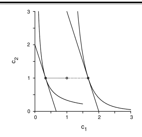
Figure 2 Agents’ Problems’ Solutions at Competitive Equilibrium with Lump-Sum Taxes Implementing the Utilitarian Optimum
0
1
2
3
1
2
3
0
c
1
c
2From (23) and (24), it is easy to see thatTH(13) = TL(13) = 0. Thus, zero taxes are optimal withγ = 13, which exactly replicates the result we obtained in the constructive proof of Theorem 1. Whenγ =0, i.e., when the society puts zero weight on welfare of the typeH, the lump-sum tax on agentsH is
TH(0)=2, i.e., all wealth is taken away from agentsH. At the other extreme,
TH(∞) = −2, i.e., the government transfers all wealth to agents H when
γ = ∞.
Figure 2 depicts the solution to the agents’ utility maximization problems at the equilibrium implementing the utilitarian optimal allocation (i.e., when all agents receive the same welfare weight in the social planning problem). Withγ =1, we haveTH(1)= −32 andTL(1)= 23. The equilibrium price is
ˆ
q(1)= 13. At this price, the ex-dividend value of each agent’s capital in period 1 is13. The after-tax wealth of typeH, thus, isy+ ˆq(γ )−TH =2, while that of typeLisy+ ˆq(γ )−TL= 23. The budget constraint for typeL, therefore,
is
c1+c2/3= 2 3,
and the optimal choice iscˆL=(13,1). TheHtype faces the budget constraint
c1+c2/3=2,
and his optimal choice is cˆH = (53,1). Figure 2 depicts these budget con-straints and optimal choices along with two indifference curves representing the maximal utility levels attained by each type in equilibrium with lump-sum taxes (TH(1), TL(1)). The pale, horizontal, solid line represents the lump-sum tax on the patient typesTL(1) = 23. The pale, horizontal, dashed line represents the lump-sum transfer to the impatient type, i.e., the negative of the taxTH(1) = −23. Under these transfers and the capital priceq(ˆ 1) = 13, the two types’ budget constraints are parallel, with the budget line of typeL
being strictly inside (closer to the origin) the budget of typeH. Agents choose
ˆ
aH = ˆaL=0.
With complete information about agents’ types, the government can freely redistribute wealth among the two types of agents. With a competitive market for capital, no further government intervention is needed for either efficiency or distributional reasons. Nondistortionary lump-sum taxes are sufficient to efficiently attain any distributional objective of the government, i.e., they im-plement any First Best Pareto-optimal allocation of consumption.
Inefficacy of Lump-Sum Taxes Under Incomplete Public Information
Suppose now that the government cannot directly observe agents’ types. Can the government implement a wealth transfer from one type to the other when it does not see which agents are of which type? Certainly the lump-sum tax system described above cannot be used because it requires the knowledge of agents’ types. Potentially, the government could elicit this information from the agents. However, if the government uses this information to simply transfer wealth, agents will not reveal their type truthfully.
This is very intuitive. The larger an agent’s after-tax wealth, the better off this agent will be in any competitive equilibrium. With agents themselves being the only source of information about their preference types, any lump-sum tax withTH =TLwill make some agents lie about their type. Clearly, if
TH < TL, everybody will declare themselves to be of typeH. IfTL < TH, everybody will say they are of typeL. Therefore, if the government sets lump-sum taxesTH =TL, all agents will end up paying min{TH, TL}, i.e., all agents will pay the same amount. Given the government budget constraint, this amount must be zero. Thus, when agents’ types are their private information, the only lump-sum taxes that the government can feasibly implement are
TH = TL = 0. We see that if the government wants to (or is restricted to) use lump-sum taxes to redistribute social surplus and agents have private information, the government can redistribute nothing.
It is worth emphasizing that the competitive equilibrium allocation re-mains efficient in our economy even when agents have private information about their type, i.e., the First Welfare Theorem holds in our economy with private information. An easy way to see that this indeed is the case is simply to check that the competitive equilibrium allocation,cˆ, given in (15)–(16) be-longs to the set of Second Best Pareto-optimal allocations characterized in G08 (see Figure 4 in particular). In fact, this is quite intuitive. Private information does not interfere with the price mechanism in our model because it does not affect the nature of the commodity that is being traded. Under both complete and private information about agents’ preferences, consumption is traded for capital. Preferences of buyers and sellers do not affect the nature of this trade beyond what is captured by agents’ demand functions. The competitive price mechanism is thus efficient.13
In sum, competitive equilibrium delivers one efficient allocation in our economy—under both complete and incomplete public information. This allocation represents a particular distribution of the gains from trade among the two types of agents. Thus, competitive equilibrium is suboptimal under almost all possible strictly Paretian social preference orderings (represented by the parameterγ ∈ [0,∞]).14 In the case of complete public information,
this distributional problem can be remedied by lump-sum taxes. In the case of private information, however, lump-sum taxes are powerless. In fact, in our economy, the only implementable lump-sum tax is the zero tax on all agents. Motivated by this, we now turn to distortionary taxes.
5. COMPETITIVE EQUILIBRIUM WITH DISTORTIONARY
TAXES
For the remainder of this article, we assume that information available to the government is incomplete. In particular, agents’ impatience is known only to them. We assume that the government knows the population distribution of the impatience parameter,θ, but cannot determine the value of θ on an agent-by-agent basis. Thus, tax systems in which the amount levied on an agent depends directly on the agent’sθ are not feasible to the government.
13 In particlular, the classic lemons problem of Akerlof (1970) does not appear in this market. 14 One could also consider non-Paretian social preference orderings (see Mas-Colell, Whinston, and Green [1995], Section 22.C). By considering only strictly Paretian social welfare functions (of the form αuH+(1−α)uL, where uθ =θ u(c1θ)+βu(c2θ) for θ=H, L) we pose a reasonably strong restriction on the set of allocations that can be considered optimal. In this restricted set, almost all Second Best Pareto-optimal allocations cannot be supported by competitive equilibrium with lump-sum taxes.
Let us start by defining a general class of feasible tax systems. For dates
t =1,2, letTt denote the mapping from agents’ publicly observable charac-teristics att to the tax payments to the government att. In the first period, agents trade current consumption for capital. These trades are observable to the government. Thus,T1(c1, a)represents the amount of tax due at the end of date one. At the end of the second date, second-period consumption is also publicly available, soT2(c1, a, c2)is the second-period tax function. Clearly, the government can use any tax system of this form because the amounts due from each agent depend only on what the government can observe. In particular,T1andT2do not depend on the unobservable parameterθ.
Under a tax system(T1,T2), agents’ budget constraints are given by
c1+qa = y−T1(c1, a),
c2 = (1+a)y−T2(c1, a, c2).
Competitive equilibrium is defined, again, analogously to Definition 1: agents optimize, markets clear, and government budget constraints are satis-fied. With taxes(T1,T2), these constraints are given by
θ=H,L μθT1(c1ˆ θ,aˆθ) = 0, (25) θ=H,L μθT2(c1ˆ θ,aˆθ,c2ˆ θ) = 0, (26)
wherecˆt θ andaˆθ are equilibrium values of agents’ consumption and capital trades.
Note that any nonzero feasible tax system(T1,T2)will be distortionary. Indeed, if a tax system(T1,T2)is not distortionary, thenT1andT2must be
constant (independent of their arguments). In this case, the government budget constraints (25) and (26) imply immediately thatT1=T2=0.
Since agents’ actions, but not types, are observable, it is clear that redis-tribution can be achieved only with taxes that depend on agents’ actions and not types. However, it is not obvious what form these taxes should take in order to be effective. The next subsection provides an example of a simple distortionary tax system that is feasible but completely ineffective for imple-mentation of redistribution.
A Simple Distortionary Tax System
In this subsection, we examine a simple tax system with a proportional tax on capital income. In this system, capital income in periodtis taxed at a flat rate
Tt.15 In our general notation, this tax system is written as
T1(c1, a) = τ1y−T1,
T2(c1, a, c2) = τ2(1+a)y−T2.
A tax system of this form consists of four numbers, (τt, Tt)t=1,2. Setting τt =Tt =0 fort =1,2 gives us the competitive equilibrium outcome, i.e., the equilibrium allocation is a Pareto optimum with the relative weight of the high type equal toγCE = 1
3. We want to study what other efficient allocations
can be achieved in this economy with a tax system of the form(τt, Tt)t=1,2.
The answer turns out to be: none.
Under taxes,(τt, Tt)t=1,2, agents’ budget constraints are given by c1+qa = y(1−τ1)+T1,
c2 = (1+a)y(1−τ2)+T2,
and the government budget constraints are
τ1y = T1,
θ=H,L
μθτ2(1+ ˆaθ)y = T2.
Because of agents’ equilibrium choices aˆθ satisfy capital market clearing θ=H,Lμθaˆθ =0, the second-period government budget constraint reduces to
T2 = τ2y(1+ θ=H,L
μθaˆθ)
= τ2y.
Thus, in both periods the amount the government refunds to each agent must equal the marginal capital income tax rate times the economy’s aggregate amount of capital income, which in our model is fixed atY =y.
Usingτ1y =T1, the agents’ budget constraint in the first period reduces to
c1+qa = (1−τ1)y+τ1y = y.
Thus, the first-period tax on capital income has no effect on the agents’budgets, as every agent has the same capital income and receives the same lump-sum refund equal to the average capital income tax.
15 Proportional distortionary taxes have been extensively studied in a vast literature initiated by Ramsey (1927). That literature concentrates on the question of minimization of the distortions resulting from proportional taxes, without addressing the question of optimal taxation. In particu-lar, that literature does not consider situations in which distortionary taxes may have a corrective function, e.g., in economies with externalities or private information.
In the second period, usingτ2y = T2, we can simplify the budget con-straint as follows
c2 = (1+a)y(1−τ2)+T2 = (1+a)y(1−τ2)+τ2y = (1+(1−τ2)a)y.
We see that the lump-sum refunded flat tax on capital income,τ2 > 0, acts
simply as a transfer from those who buy capital (a >0) to those who sell it (a <
0). Ifτ2 <1, this transfer is proportional to the amount of capital traded.16
We note here that in a regular capital market transaction the payment that the buyer makes to the seller is a transfer of the exact same form. In particular, the tax payment,τ2a, just like a price payment, is proportional to the amount,
a, of capital being traded. From this observation, we see that a proportional tax on capital, withτ2<1, does nothing but change the equilibrium price of
capital. In particular, under any tax of this form, equilibrium allocation will coincide with the competitive equilibrium allocation,cˆ, so no redistribution can be achieved.
To see this point more clearly, let us write the agents’ budget constraints again in the present-value form. From the first-period budget constraint we have thata =(y−c1)/q. Substituting into the budget constraint at date two, we obtain
c2=(1+(1−τ2)(y−c1)/q)y,
which is equivalently written as
c1+c2 q (1−τ2)y =
q
1−τ2 +y.
Let us now denoteq/(1−τ2)byQ. This value represents the tax-adjusted price of capital. Foranytax rateτ2<1, we can write the present-value budget
constraint as
c1+c2Q/y=Q+y,
which is the same expression as the budget constraint agents face in the model without taxes, but with the price of capital,q, replaced with the tax-adjusted price,Q. The solutions to these two models must therefore be the same, i.e.,
ˆ
Q= 12. Thus, under a proportional capital tax, the equilibrium price of capital isqˆ =(1−τ2)/2 and the unique equilibrium allocation iscˆforanytax rate,
τ2<1.
This result is intuitive. Absent taxes, qy is the price of one unit ofc2 in terms ofc1. With tax,τ2, on capital purchases,a, in order to obtain one extra
16 If τ2=1, the government taxes the proceeds from the sale of capital at the rate of 100
percent. Under this tax, the market for capital is shut down, the tax proceeds are zero, and the only equilibrium is autarchy, which is not an efficient allocation in this economy.
unit ofc2, an agent must purchase 1/(1−τ2)y units of capital at date one. With the price of capital beingq, this means that it takesq/(1−τ2)y units ofc1to purchase one unit ofc2. The benefit of selling capital in period 1 is symmetrically increased, as selling capital now not only brings in resources for consumption today but also saves capital income taxes tomorrow. By affecting both sides of a capital transaction symmetrically, the tax,τ2, changes
the nominal price of capital but does not change the real tradeoff that agents face in equilibrium.
Setting aside the case of complete market shutdown, we see that no distor-tionary tax system of the form(τ , T )can affect the competitive equilibrium outcome. For any marginal tax rate, τ2 < 1, the equilibrium allocation is
the same as it is forτ2 = 0. In the next section, we consider distortionary
tax systems capable of changing the equilibrium outcome and implementing other efficient allocations.
6. EFFICIENT REDISTRIBUTION WITH DISTORTIONARY
TAXATION UNDER INCOMPLETE INFORMATION
In this section, we devise a class of tax systems that are feasible despite agents’ private information and capable of implementing any Second Best Pareto-optimal allocation. Similar to the simple system (τ , T ) considered in the previous section, we will have a distortionary tax on capital and a lump-sum component. However, the distortion will not affect both parties to a capital sale/purchase transaction symmetrically.
An Optimal Distortionary Tax System
The tax system we consider in this section consists of two parts. First, there is a lump-sum tax,Tt, levied on all agents in periodt =1,2. Second, there are subsidies to sufficiently extreme capital trades. The form these subsidies take is as follows. The government sets a (negative) threshold,a, and pays a subsidy,S1−, in period 1 to all agents whose capital purchases are not greater
thana (i.e., a subsidy to all who sell a sufficiently large quantity of capital). Alternatively, the government can set a threshold,a, and pay a subsidy,S2+, in period 2 to all agents whose capital purchases are not smaller thana(i.e., a subsidy to those who buy a lot of capital). In the tax system implementing a given Second Best Pareto optimum, only one of these subsidies will be nonzero.
A tax system of this form is therefore given by six numbers(T1, S1−, a, T2, S2+, a). In the general notation introduced in the previous section, we can express this tax system as follows:
T1(c1, a) = T1−Ia(a)S1−, (27)
whereIaandIaare indicator functions given by Ia(a)= 1 if a ≤a, 0 otherwise, and Ia(a)= 1 if a ≥a, 0 otherwise.
We restrict attention to this class of tax systems because, as we will show, taxes in this class are sufficient for implementation of all Second Best Pareto-optimal allocations. In the next section, we discuss the possibility of imple-menting Second Best Pareto optima with other tax mechanisms.
Clearly, since taxes (27)–(28) do not depend on the unobservable param-eterθ, agents of both types face the same budget constraint, which is given by
c1+qa ≤ y−T1+Ia(a)S1−, c2 ≤ (1+a)y−T2+Ia(a)S2+.
Also, the government budget constraints (25)–(26) can be expressed as
θ=H,L μθS1−Ia(aˆθ) = T1, θ=H,L μθS2+Ia(aˆθ) = T2.
As before, competitive capital market equilibrium with taxesT =(T1, S1−, a, T2, S2+, a)consists of a consumption allocation, cˆ =(c1ˆ H,c1ˆ L,c2ˆ H,c2ˆ L); capital trades,aˆ =(aˆH,aˆL); and a capital price,qˆ, such that (i) agents opti-mize, i.e., the equilibrium allocation maximizes agents’ utility given the price,
ˆ
q, and taxes,T; (ii) the capital market clears; and (iii) the government’s budget is balanced in every period. As before, we will say that the tax system,T, im-plements a Second Best Pareto optimum,c∗∗(γ ), if there exists a competitive equilibrium such thatcˆ=c∗∗(γ ).
Analogous to (19), letm∗∗θ (γ )denote the intertemporal marginal rate of substitution of agents of typeθ at the Second Best Pareto optimum,c∗∗(γ ), i.e., m∗∗θ (γ )= βu (c∗∗ 2θ(γ )) θ u(c∗∗1θ(γ )) .
The following result is a version of the Second Welfare Theorem with private information.
Theorem 3 Every Second Best Pareto optimumc∗∗can be implemented as a competitive equilibrium with taxes,T. In particular, forγ ∈ [0,∞], the Second Best Pareto optimumc∗∗(γ )is implemented by the tax system
given as follows. Forγ < γCE : T1(γ ) = S1−(γ )=a(γ )=0, T2(γ ) = Y −c∗∗2H(γ )+m∗∗H(γ )− 1 Y −c∗∗2L(γ ) , S2+(γ ) = c∗∗2L(γ )−c2∗∗H(γ )+m∗∗H(γ )− 1 c1∗∗L(γ )−c∗∗1H(γ ) , a(γ ) = Y m∗∗H(γ )−1Y −c∗∗1H(γ ). Forγ ≥γCE: T2(γ ) = S2+(γ )=a(γ )=0, T1(γ ) = Y −c∗∗1L(γ )+m∗∗L(γ ) Y −c2∗∗L(γ ) , S1−(γ ) = c1∗∗H(γ )−c1∗∗L(γ )+m∗∗L(γ )c∗∗2H(γ )−c∗∗2L(γ ), a(γ ) = Y−1(c∗∗2H(γ )−Y ).
Although the expressions for the thresholds and transfers specified in the tax system,T(γ ), look complicated, the intuition behind them is very simple. Absent taxes, as we have seen, the competitive market mechanism implements the efficient allocationc∗∗(γCE). In order to implement an optimumc∗∗(γ )for someγ > γCE, the government must redistribute from the patient types,L, to the impatient types,H, (recall thatγ is the relative weight that the impatient type,H, receives in the social welfare objective). How can this redistribution be achieved when the government cannot observe agents’ types?
In competitive equilibrium without taxes, the impatient types sell capital because of their strong preference for first-period consumption. The patient types buy it. Thus, the government knows ex post who the impatient and pa-tient agents are simply by looking at agents’ capital trades. Suppose then that the government, targeting the impatient agents, gives a small subsidy to those who sell a sufficiently large quantity of capital. If the subsidy is small enough, or the minimum sale size requirement is sufficiently large, this subsidy will not cause the patient agents to change their behavior (i.e., to flip from buying to selling capital).17 Under such a subsidy, patient agents still buy capital and,
therefore, do not collect the subsidy. The impatient agents, who were selling capital even without the subsidy, continue to sell it, which now gives them the additional benefit of the subsidy. Thus, the subsidy reaches the targeted type. If this subsidy is funded by lump-sum taxes on all agents, it redistributes from the patient agents to the impatient ones, as intended. The optimal tax mech-anism,T(γ ), delivers the subsidy to the targeted type precisely in this way. For anyγ > γCE, the optimal tax system,T(γ ), provides a threshold level,
a(γ ), and a subsidy level,S1−(γ ), that achieve in equilibrium the amount of
17 In the language of mechanism design, the market mechanism distorted by such a subsidy remains incentive compatible.
redistribution (relative to the competitive market allocation) required to im-plement the optimal allocation,c∗∗(γ ).
Similarly, in order to implement the optimumc∗∗(γ )for someγ < γCE, the government redistributes from the impatient types,H, to the patient types,
L.Taxes, T(γ ), are again designed to not induce the agents to flip, so the impatient types continue to sell capital and the patient types continue to buy it. Forγ < γCE, the lump-sum-funded subsidy,S+
2(γ ), goes to the buyers
of capital, that is typesL, and thus reaches the targeted type of agent. In this way, taxT(γ )achieves the desired redistribution.
Let us now argue slightly more formally that this intuition is consistent with equilibrium. We need to demonstrate that conditions (i)–(iii) defining competitive equilibrium with taxes are satisfied under taxes,T(γ ), with con-sumption,cˆ=c∗∗(γ ), along with some prices,q(γ )ˆ , and capital trades,aˆθ(γ ). More precisely, we will argue that equilibrium capital price,q(γ )ˆ , can be ob-tained from the IMRS of the agents who do not receive the subsidy to capital sales/purchases. Forγ > γCE, these are the patient agents, i.e.,
ˆ
q(γ )=m∗∗L(γ )y (29)
for theseγ. Forγ < γCE, the impatient types do not receive the subsidy, thus
ˆ
q(γ )=m∗∗H(γ )y
for allγ in this range. The subsidy threshold levelsa(γ )anda(γ )are such that the following capital trades are optimal in the agents’ utility maximization problem: ˆ aH(γ ) = a(γ ), ˆ aL(γ ) = − μH μL a(γ )
for eachγ > γCE, and
ˆ aH(γ ) = − μL μH a(γ ), ˆ aL(γ ) = a(γ ) for eachγ < γCE.
Checking that equilibrium conditions (ii) and (iii) are satisfied amounts to a bit of simple algebra. The crux of the argument is in checking the first equilibrium condition, i.e., in showing that under taxes,T(γ ), and proposed equilibrium prices,q(γ )ˆ , agents of typesH andLindeed find it optimal to choose the proposed equilibrium capital tradesaˆH(γ )andaˆL(γ ), respectively. An algebraic proof of this result would be very tedious. In particular, note that the algebraic argument we used in the case of lump-sum taxes with full information cannot be used here, as the Euler equations are invalid due to the budget line being given by a non-differentiable function.
We will thus proceed differently. For several selected values ofγ, we will demonstrate graphically that the optimal allocationc∗∗(γ )is consistent with
agents’individual utility maximization under taxes,T(γ ). Qualitatively, these values will be representative of the whole spectrum ofγ. From our graphical argument, it will be clear that the conclusion holds for allγ ∈[0,∞].
Consider the case ofγ =1 (which represents the utilitarian social welfare objective). Since 1> γCE= 1
3, we have that the tax system,T(1), provides a
subsidy,S1−(1), to agents whose capital purchases,a, are not larger thana(1).
From the closed-form expression forc∗∗(1)given in equations (21)–(22) of G08, we have that the optimal utilitarian allocation hasc∗∗H(1) =(32,12)and
c∗∗L(1)=(12,32). Substituting these values into the formula for tax parameters
T(1)given in the statement of Theorem 3, we have
T2(γ )=S2+(γ )=a(γ )=0 and T1(1) = 1 3, S1−(1) = 2 3, a(1) = −1 2.
Under the tax system,T(1), therefore, agents who sell at least half of their initial capital stock receive the subsidy of 23units of consumption at date one. There is no subsidy to buying assets. All agents pay the lump-sum tax of 13at date one. From (29) we compute
ˆ
q(1)= 1
3.
The thick crooked line in Figure 3 represents the budget constraint that all agents face in their utility maximization problem under taxes,T(1), and price, q(ˆ 1). The horizontal segment of this budget constraint results from the subsidy,S1−(1). The horizontal dashed line represents the lump-sum tax,
T1. The two convex curves in Figure 3 are the highest indifference curves that typesH andLattain in their utility maximization problems under taxes,
T(1), and price, q(ˆ 1). The indifference curve of type H has exactly one point in common with the budget constraint,c∗∗H(1)=(32,12). The impatient agents, therefore, maximize their utility by choosing the consumption pair
c∗∗H(1), which is consistent with implementation of the Second Best Pareto optimumc∗∗(1). The indifference curve of typeLmeets the budget constraint at two points:c∗∗L(1)=(12,32)andc∗∗H(1)=(32,12). Thus,c∗∗L(1)is consistent with the individual utility maximization of theLtypes, as well, however not uniquely.18
18 That this individual optimum is not unique is necessary in the implementation of the optimum c∗∗(1) because the incentive compatibility constraint of type L, (6), binds at c∗∗(1).
Figure 3 Individual Optima of the Two Types Under the Budget Constraint Resulting from Taxesτ (1)
0
1
2
3
1
2
3
0
c
1
c
2Note in Figure 3 that the indifference curve of typeHis flatter atc∗∗H(1)= (32,12)than the downward-slopping segment of the budget constraint at this point. This is a consequence of the so-called intertemporal wedge, which is described in detail in G08. The slope of the budget line, everywhere outside of the horizontal segment, equals−m∗∗L(1)−1. The slope of the indifference curve of theH type at c∗∗H(1)is−m∗∗H(1)−1. Because of the intertemporal wedge
prevailing at the optimal allocationc∗∗(1), these two rates are not equal. In fact, the sloping segment of the budget line is strictly steeper than the indif-ference curve of theH type atc∗∗H(1). This implies that the optimal subsidy,
S1−(1), could not be made available with a weaker capital sale requirement than
Non-uniqueness for at least one type of agent will appear in any implementation of any Second Best