Road environment modeling using robust perspective analysis
and recursive Bayesian segmentation
Marcos Nieto • Jon Arróspide Laborda • Luis Salgado
Abstract Recently, vision-based advanced driver-assistance systems (ADAS) have received a new increased interest to enhance driving safety. In particular, due to its high perfor-mance-cost ratio, mono-camera systems are arising as the main focus of this field of work. In this paper we present a novel on-board road modeling and vehicle detection system, which is a part of the result of the European I-WAY project. The system relies on a robust estimation of the perspective of the scene, which adapts to the dynamics of the vehicle and generates a stabilized rectified image of the road plane. This rectified plane is used by a recursive Bayesian classi-fier, which classifies pixels as belonging to different classes corresponding to the elements of interest of the scenario. This stage works as an intermediate layer that isolates sub-sequent modules since it absorbs the inherent variability of the scene. The system has been tested on-road, in different scenarios, including varied illumination and adverse weather conditions, and the results have been proved to be remarkable even for such complex scenarios.
Keywords ADAS • Real-time • Plane rectification • Bayesian segmentation • Kalman filtering • Multi-domain vehicle tracking
1 Introduction
On-board advanced driver-assistance systems (ADAS) have been receiving increasing attention from the intelligent trans-portation system (ITS) community (car manufacturers, M. Nieto (£3) • J. Arróspide Laborda • L. Salgado
Grupo de Tratamiento de Imágenes,
Universidad Politécnica de Madrid, Ciudad Universitaria s/n, ETSIT C-306, 28040 Madrid, Spain
e-mail: [email protected]
research centers and users) due to their ability to provide useful information about the vehicle environment by func-tioning as sensors for services such as lane departure warning, collision avoidance, stop-and-go, etc. In particular, the solu-tions based on video processing have played an important role in this field since the past decade, due to their low cost, the increased performance of microprocessor systems, and the research advances in the field of computer vision [1].
The on-board scenario poses a number of challenges for vision systems, as it is an extremely varied environment [2]. For instance, it involves sudden and significant illumination changes (as when entering into tunnels), different types of road pavement, or the appearance of lane markings, which may have contrasts that vary significantly from one road to another. Moreover, weather conditions may also affect vision systems. For example, the image could contain rain drops, moving wipers, etc. Additionally, the motion of the scene entails more complexity, as it is composed of the motion induced by the vehicle itself with respect to static elements, and of other vehicles, typically moving at different speeds.
The most recent trends in this field have focused on 3D environment modeling using stereovision systems, due to their ability to recover depth information from the analy-sis of two synchronized video inputs. For instance, several works address sub-pixel accuracy lane markings models
[3-5] using calibration information. Others use image align-ment between the stereo pair to detect volumetric objects on the road plane [6,7], or to enhance lane marking detection [8]. While showing promise in obtaining depth information, stereoscopic vision has a number of drawbacks: multi-view systems are typically not considered for real-time applica-tions due to their built-in complexity, which is mainly related to the calibration process, the necessity of a synchronized acquisition system, and the difficulties encountered in finding reliable correspondences between images [9]. Mono-camera
systems are more cost-effective and hence more widely used in real applications [10]. Different mono-camera approaches have been proposed in the literature to address the road mod-eling [11], including accurate lane markings models [12,13],
and vehicle detection and tracking [14-17].
Some of these solutions provide coarse or incomplete results due to the intrinsic limitations of the mono-camera analysis: projective geometry is typically handled using appearance-based methods that may be faster than stereo [18]
without evaluating the loss in robustness. However, some researchers compensate for this limitation by making prior assumptions about the environment, for example, by denn-ing a constant relative pose of the camera with respect to the road [11,19]. However, such approaches reduce the system's capability to adapt to more realistic situations.
In this paper we propose a new mono-camera system, which is the result of the research work carried out during the European I-WAY project. It provides an accurate and very complete environment model that dynamically adapts to changes in the scenario and that minimizes the use of prior information. This approach comprises robust strategies that ensure reliable real-time operation in real driving situations. Our approach is fully adaptive to the unknown scenario conditions, without using prior information about the pose of the camera with respect to the road, which as opposed to most approaches in the literature is automatically retrieved through an adaptive computation of the image-plane to road-plane homography [2,20]. This transform, which is stabilized using a dynamic vanishing point estimation method, removes the inherent perspective distortion from the images and thus simplifies further analysis stages.
The adaptability to the extremely variable on-road envi-ronment is given by a MAP probabilistic framework, which is the major contribution of this paper, since it allows to inte-grate models of different elements of the road altogether in a simple way, allowing to overcome the need to handle multiple detectors for each targeted element (vehicles, lane markings, pavement, etc.). This framework operates on the transformed domain and segments the elements of the road according to a set of dynamic likelihood and prediction mod-els that are updated through the observation of different fea-tures extracted from the images. This stage can be seen as a layer that absorbs the dynamism of the input images, includ-ing illumination changes, rapid motion objects, or sudden changes of the appearance of the road. The output are steady segmented images that facilitate the subsequent modeling tasks, which do not have to care about the complexity of the observations.
The description of the road environment delivered by the modeling stages takes into consideration a wide variety of useful information for ADAS. This information is related to both static and dynamic elements of the environment, e.g., the lanes and their geometry, and mainly, the vehicles on the
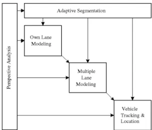
Adaptive Segmentation Own Lane Modeling Multiple Lane Modeling Vehicle Tracking c
Fig. 1 Block diagram of the proposed Road Modeling system
road. These elements are described using appearance-based models that are dynamically updated through stochastic fil-tering, which enhances the accuracy and completeness of the results. Most remarkably, a cooperative analysis of the original and transformed domain is exploited to overcome the intrinsic limitations of each domain.
The system has been tested on-road, and has proved to perform in real-time and to provide accurate and reliable results for a set of different environments, including variable illumination and adverse weather conditions, heavy traffic, different types of roads, different pavement colors, etc.
2 System overview
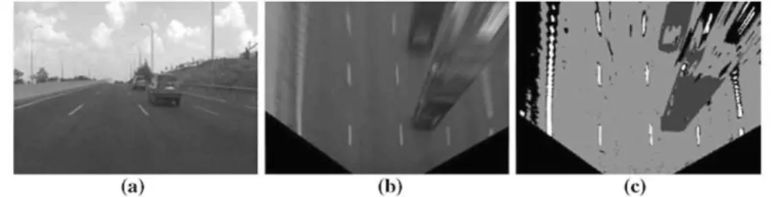
The system aims to provide a full description of the scenario ahead of the vehicle, i.e., a model of the road and the vehicles in it, in real-time. The block diagram of the system is shown in Fig. 1. The processing is divided into three core blocks: perspective analysis, recursive Bayesian segmentation, and scene modeling. For each incoming image, the geometry of the scene is analyzed in order to derive a transformation that removes perspective distortion from the image. As a result, a fronto-parallel view of the road ahead is obtained in which road elements (i.e., lane markings) and vehicle dynamics are proportional to their real appearance and behavior, as shown in Fig. 2. Then, the image in the transformed domain is seg-mented through a Bayesian classifier that uses a parametric multiple-class likelihood model of the road. The pixels in the image are thus classified as belonging to pavement, lane markings, dark objects or to unknown elements not classifi-able as any of the previous (see Fig. 2c).
In the final stage, a full description of the scene elements is provided, using the information obtained in the segmentation image and the defined models. This stage consists of two par-allel analysis modules: road modeling and vehicle detection
Fig. 2 Segmentation process: a original image; b road-plane; and c four-level segmentation (in black for unknown elements)
and tracking. In the former, novel lane tracking and model fitting techniques allow to obtain precise information of the own and adjacent lanes. In turn, vehicle detection and track-ing strategy relies on a collaborative approach between the original and the transformed domains. Additionally, a feed-back loop allows to use vehicle detection results as an input for segmentation of the following images, thus exploiting their underlying temporal coherence. Eventually, the output of both modules is combined to produce high level informa-tion, such as detections of lane changes of the own or other vehicles, vehicle trajectories, etc.
3 Perspective analysis
An important perspective distortion arises in images cap-tured from cameras moving in the direction of the optical axis, as shown in the example in Fig. 2a. There are a num-ber of benefits derived from the removal of this effect in road scenarios, available through the computation of a virtual fronto-parallel view of the road ahead (typically denoted as "bird's-eye view" or "Inverse Perspective Mapping") [2,21]:
lane markings are parallel in this domain, lanes are imaged with their actual width (up to scale), the complexity of the curve analysis is reduced and also the relative speed and position of the vehicles are imaged without distortion, with magnitudes proportional to the actual ones on the road.
Many works, especially the former on plane rectification [2], assumed the prior knowledge of all the parameters of the projective matrix: i.e., the camera calibration matrix as well as the relative rotation and translation of the camera with respect to the road plane.
These type of assumptions might be valid for surveillance systems that do not model the dynamism of the road scenario, but in on-board systems it can lead to large errors in the rec-tification, due to the steering of the vehicle, its bumping, or slope changes. Some authors have studied the dependence of the obtained transform image according to the variability of the environment. For instance, [31 ] analyzes the impact of the pitch and yaw angles in the obtained rectified image in terms of radial distortion and parallelism. In this line, differ-ent authors have iddiffer-entified the pitch angle error (i.e. the error between the instantaneous pitch angle and that used to
per-form rectification), as the main cause of the image distortion, and have proposed methods to minimize this error. Jiang [18]
computes the rectification with fixed parameters and checks the parallelism between the left and right lane markings, esti-mated as straight lines, corrects the angles, and re-estimates the rectification. Cerri [30] computes several rectifications using a range of pitch values, and then also checks the par-allelism between the detected lane markings to determine which pitch angle was the correct one.
In this work, we propose to update the values of both the pitch and yaw angles at each time instant by means of the robust computation of the dominant vanishing point of the scene, given by the intersection of the lane markings. Hence, in contrast to most approaches our method represents a flexible and robust alternative to perform plane rectification. 3.1 Pinhole camera projection
The projection process that generates the image shown in Fig. 2b is described as a linear process using homogeneous coordinates for both the points in the 3D space and the image coordinates [22]. If we define a point in the 3D world as X in homogeneous coordinates, its projection into the image plane combines two transforms: the former converts the point into the camera coordinate system, yielding Xc, and the second
projects it into the image plane, x. The combination of these steps renders the following expression:
x = KXC = K(R| - Rc)X = PX (1)
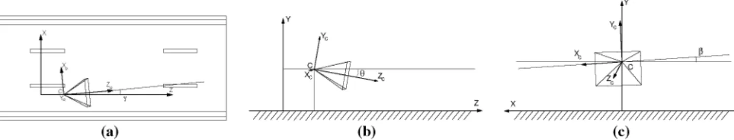
where P is the so-called projection matrix, K is the cam-era calibration matrix, and R and c are the aforementioned relative rotation and translation, respectively, between the world and camera coordinate systems. These concepts are illustrated in Fig. 3.
If we now consider points in the 3D space that correspond to the road plane (i.e., with spatial coordinate Y = 0), and define p¿ as the i-th column of P we arrive at the following expression:
0
z
vi y
(a)
//////////y//////////////////////////
(b) (c)
Fig. 3 Yaw (y), pitch (9) and roll (f¡) angles, respectively in a, b, and c within the defined road scenario. The camera coordinate system is shown a s { Xc, 7c, Zc}
which yields the target plane to plane homography H between the coordinates of the points of the road plane, x', and the points on the image plane, x.
Therefore, we can compute the homography that leads to the rectified domain by computing the unknown parameters of the projection matrix P, which are, in our case, the rota-tion angles. The rest of parameters can be considered fixed and known, like the camera calibration matrix K, which is computed off-line, and the translation c, as the camera moves rigidly with respect to the vehicle.
Since the camera is installed inside the vehicle with null roll angle, the problem is significantly simplified. This assumption holds if the camera is carefully installed without rotation with respect the Z-axis, and implies that the horizon line is actually horizontal. Hence, if we determine the posi-tion of the horizon in the image (by estimating its coordinate in the y-axis), we have recovered the affine properties of the plane, e.g., parallelism, area ratios, as well as the angular information, provided that we know the camera calibration matrix.
This way it is enough to compute the vanishing point asso-ciated with the lane markings of the road, that we will call
vz = (uz,i> vz,2, 1)T, which belongs to the line at the
infin-ity and thus defines it completely. The computation of the vanishing point is addressed in the following section.
The vanishing point is then projected into the camera
coor-dinate system as v' = K_ 1v2, so that thepitch and yaw angles 3'2 V a n i s h i n8 Po i n t estimation
obtain v^ = (tan y cos 6, tan 0, 1)T, which are two equations
on the two unknowns 6 and y, solved using the Eq. (3). Figures 4 and 5 show two example sequences represent-ing two typical situations. The former depicts a lane change manoeuver, where the vehicle is steering at the right and makes two consecutive lane changes. As shown in Fig. 4,
the height of the vanishing point, vz^ is almost constant,
apart from some detection noise, and so is the pitch angle. The transversal position of the vanishing point, vZti, changes,
indicating a significant change of the yaw angle. This is max-imum when the vehicle is at maxmax-imum steer, and returns to its initial values as the vehicle stabilizes its position within a lane.
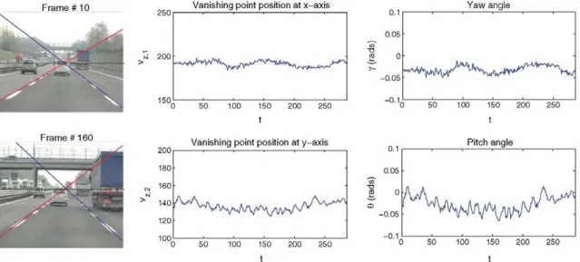
The second example, shown in Fig. 5 illustrates the behav-ior of the vanishing point in a significant road slope. Thepitch angle is the one that varies more significantly, following the movement of the vertical component of the vanishing point, vZt2- The yaw angle is steady, since although it depends on the
variation of the pitch angle, its influence is highly attenuated by the arctangent expression shown in Eq. (3).
As a result, we obtain rectified images of planes which show parallel lane markings, with constant width, even in difficult situations where the described extrinsic parameters vary.
can be directly computed as 0 = arctan(^ 2); Y = arctan
y cose J (3)
These expressions come from the following argument: consider the point at the infinity corresponding to the van-ishing point \z, and its projection into the image plane as
K(R| - Re) 0 1
voy
(4)
so that if we consider that we know the camera calibration matrix and we left-multiply both sides of (4) by K_ 1 we
As stated in the previous section, the correct estimation of the vanishing point along time is a key step towards the adapt-ability and stadapt-ability of the system. For this purpose, we have designed a robust method for vanishing point estimation. It is based on a specific lane marking detector that pro-vides instantaneous measurements about the vanishing point, and on a Kalman Alter that provides temporal coherence to the measurements, and also allows to control the putative outliers.
Lane markings can be approximated as straight lines in the lower part of the image, even in the presence of significant curvature ahead. The detection is done using a specific lane marking detector, which is applied to each row of the image, assuming that the appearance of the lane markings in this
Frame # 4 Vanishing point position at x-axis Yaw angle
0 50 100 150 200 250 300 I
Vanishing point position at y-axis
0.1 0.05 0 -0.05 -0.1 0 50 100 150 200 250 300 I Pitch angle V \ y v / \ v V W W * ^ / 4 / \ T ^ ^ 0 50 100 150 2 0 0 2 5 0 3 0 0 t
Fig. 4 Example of variation of the pitch and yaw angle in a lane change manoeuver. The vanishing point is shown as the intersection of two colored
lines for a better visualization (color in online)
Frame #10 Vanishing point position at x-axis
- ~ < v M N N v> y w f v^ r ^ ^ 0.1 0.05 "D ¡0 0 - 0 . 0 5 Yaw angle
J^
Frame #160 0 50 100 150 200 250 tVanishing point position at y-axis
-0.1
- ^ v y A ^ / ^ K w u ^ i1* ^ ^
0 50 100 150 200 250 I
Pitch angle
Fig. 5 Example of variation of the pitch and yaw angle in a road slope change
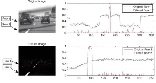
one-dimensional domain is given by pulses of high intensity values surrounded by darker regions. Therefore, the analysis is done by independently Altering each image row of inten-sity values, denoted as {x¿ }¡L1, resulting in a new Altered data
array {yi}¿=v deAned as
y i = 2Xi - (Xi-r + Xi+r) - \Xi Xi+t\ (5) where x is the width parameter that governs the Altering pro-cess. This Alter produces high responses for positions with Xi values that are higher than those of their neighbors on the left and right at a distance r. The last term in (5) penal-izes cases in which the difference between the left and right neighbors is high, so that a higher response is given to posi-tions with similar left and right neighbors. This last term makes this Alter less prone to errors than other lane marking
detectors presented in the literature [2,20]. An example is given in Fig. 6: the original and Altered images of a typical road scene are shown, and two different rows are analyzed, showing both the intensity of the original image and the result of the Alter in each row. Row 2 exempliAes the excellent per-formance of the detector, even with obstructing elements, such as the wiper of the vehicle. The scenario of Row 1 is more challenging, as there are several abrupt changes in the intensity proAle, due to the presence of vehicles. Neverthe-less, as shown in the response proAle, our method accurately detects the lane marking of interest and dismisses the super-Auous information.
The well known Hough transform [23] is then used to detect lines in the resulting image. This transform is robust against outliers and provides multiple line Atting. Each line
Fig. 6 Lane marking detector example. For clarity, the response to the filter has been normalized between 0 and 1
Original image
f
— Original Row 2— Filtered Row 2 "
Original image Filtered image
Fig. 7 Hough transform applied to the image result of the lane marking detector: a least squares vanishing point depicted as the intersection of the red lines; and b a zoom of a lane marking for which several lines have been fitted (color in online)
wheres= (sin0o, • • •, sin (9;_i)T, c=(cos0o, • • •, cost9/_i)T,
p = (po, • • •, Pi-i)T, and I is the number of lines. The least
squares solution is obtained with SVD. Figure 7 shows an example of the computation of the vanishing point for a typ-ical road scene.
Each instantaneous estimate of the vanishing point obtained, as described earlier, is treated as a noisy measure-ment, which is then introduced into a Kalman Alter to provide a better estimation of the vanishing point.
Briefly, this approach stabilizes the coordinates of the detected vanishing point by adding temporal coherence to the estimation process. The dynamic model used is a constant-velocity model, with the state vector s¿; = (vx, vy, vx, vy)T.
This model is explained in more detail in Sect. 5.1.
is parameterized with an angle 6 and a distance p as x sin 6 + y cost? = p.
The Hough transform may give more than two lines for each lane marking, which result in multiple intersection points, as shown in Fig. 7. We apply here a robust scheme that allows us to Alter the lines delivered by the Hough trans-form, in order to remove the putative outliers that would significantly affect the least squares solution. The RANSAC algorithm is used to classify lines into inliers and outliers. This algorithm works iteratively, by selecting, at each iter-ation, a pair of lines and computing its intersection point. The lines whose distance to this point are less than a given error threshold are computed as inliers, and denoted as the consensus set of the hypothesis. RANSAC iterates until the probability of finding a better consensus set is below some convergence threshold (typically 5%).
This way, the outliers are removed from the set of lines, and we can compute the vanishing point \z, without risks, as
the solution of the system of equations built with the equa-tions of each detected line:
[s I c ] v (6)
4 Recursive Bayesian segmentation
The segmentation algorithm used in this work is based on the Bayesian decision theory. The algorithm defines a paramet-ric multiple-class likelihood model of the road, from which pixels are classified into different classes, with an associated probability of error.
Three types of elements of interest are considered within any road-plane image:
- Pavement: light gray regions of the road.
- Lane markings: bright stripes painted on the road. - Objects: dark elements, such as the lower parts of
vehicles, their wheels, shadows, etc.
The probabilistic framework handles all the available information in a simple and robust way, by defining the prior probabilities and the likelihood models, and by appropriately choosing the features that best characterize the classes that are to be identified. Therefore, it avoids defining and com-puting a large amount of deterministic cases or situations
Fig. 8 Example of the application of the Bayesian classifier to the transformed domain: upper row contains images corresponding to very different scenarios; and lower contains the segmented images. Note that the result is very accurate for all of them, except for the tunnel sequence,
in which the sudden illumination changes makes the classifier to set to unknown most of pavement pixels. Nevertheless, this does not affect either the lane markings or the vehicle detection stages
regarding illumination conditions, presence of vehicles, motion, etc.
Besides, classical approaches tend to classify pixels as strictly belonging to one of the aforementioned elements. In contrast, we make use of an additional "unknown" class, which gathers the pixels which do not match the models defined for the sought elements. This is quite frequent in out-door uncontrolled environments, where additional elements such as median stripes or guard rails can appear. The pro-posed method considers these cases and hence avoids classi-fication error.
4.1 Bayesian framework
Let S = {P, L, O, U} be the set of classes that represent, respectively, the pavement, lane markings, objects, and the unidentified elements. The target of the classifier is to assign one of these classes to each pixel of the image.
Let Xi represent the event that a pixel, indexed with its spatial coordinates inside the image (x, y), with an associated observation vector denoted as zxy, is classified as belonging
to the class / e S. Using the Bayesian decision theory, this classification is carried out by selecting the class that max-imizes the a posteriori conditional probability P(Xi\zxy),
which is decomposed by the Bayes' rule as
P(Xi\Zxy) (7)
Pilxy)
where p(zxy\Xi) is the likelihood function, i.e., the
proba-bility that a pixel, according to its associated measurements, belongs to class /; P{X{) is the prior probability of each class and P(zxy) is the evidence, computed as P(zxy) =
X i s s P(zxy\Xi)P(Xi), which is a scale factor that ensures
that the posteriors sum to unity.
The result, for each pixel, is a set of posterior probabili-ties {P (Xi | zxy )}¡ ss , which denote the probability that a pixel
belongs to each defined class. Accordingly, each pixel of the image is classified as the class with the maximum poster-ior probability. The likelihood and the prposter-ior probabilities are computed as described in the following subsections.
Figure 8 shows the resulting four-level segmentation for a number of example images. As shown, the segmentation is applied to the road plane image after the perspective trans-form is computed. In the segmented image, for clarity, the pixels have been colored according to their classification: the white pixels belong to the lane markings, the light gray pixels are those that likely belong to the pavement of the road, and the dark gray pixels are those that are assigned to the wheels and shadows of the lower parts of the vehicles. The black pixels are those that have not been classified as belonging to any of the three previous classes, and therefore remain as unknown pixels.
4.2 Likelihood models
In this section the likelihood models are described as para-metric functions, according to the expected properties of the considered image features with respect to the defined classes. Additionally, the estimation of their parameters is obtained through an optimization process using the Expectation-Maximization (EM) algorithm.
The basic appearance of the defined classes may be described as follows: the pavement is usually a homogeneous area in the transformed image, sharing a common intensity level with low variations among pixels; the lane markings are represented as near-vertical bright stripes, usually sur-rounded by pavement pixels; and objects typically can be characterized by dark regions with intensity levels lower than the pavement (note that even white vehicles contain dark areas in their lower part due to shadows and wheels).
Fig. 9 Initialization of the parameters of the likelihood function for the intensity feature
Rectified plane Edge mask Pavement pixels Lane markings pixels Object pixels
With this information, it is possible to design pixel-level features that help to differentiate between classes. Two fea-tures have been used for this purpose: the intensity or grayscale level, Ixy, and the response to the lane marking
detector, Lxy. The combination of these features ensures a
clear class differentiation, especially accurate for the lane markings class, thus allowing to reduce misclassiflcations. The likelihood function of class / is defined as the product of the likelihood functions for each image feature assumed to be conditionally independent: p(zxy\Xi) = p(Ixy\Xi)
P(LXy\Xt).
4.2.1 Intensity feature
The likelihood functions for Ixy are all defined as normal
distributions. In particular, the likelihood of the pavement class is P(hy\Xp) oc exp ( -1 2 0
1 p
a
xy M,P) ) (8) where /xpp and ojyp are the mean and standard deviation ofthe distribution. The likelihood distributions of the other clas-ses are parameterized analogously as {/U./,L,<7/,L}, {/"-/, o, 07,0} and {/u./,c/, cr¡,u}- Note that there is an implicit neces-sary condition that must be satisfied: /xpo < I¿I,P < I¿I,L, since the dark objects are always darker, as well as lane mark-ings are always clearer than the pavement. The model for the unknown class is defined as a normal distribution with large fixed variance, so that it is similar to a uniform distribution. 4.2.2 Lane marking detector
Regarding the likelihood functions associated with the pro-posed detector, lane markings are expected to provide high response values to the filter and low response values for the other classes. This way, the likelihood functions for Lxy are
defined as normal distributions. The parameters of the distri-butions are {H.L,P,VL,P}, {^L,L,OL^}, {/XL I 0,CTL I 0} and
{/¿L,U,(?L,U}- The unknown class must be modeled with wide normal distribution, in the same manner as explained for the intensity feature.
For this feature, the conditions are HL,O < Í¿L,L and I¿L,P < I¿L,L, which mean that lane markings have always higher values for this feature than pavement and dark objects. 4.2.3 Parameters estimation
The parameters of the aforementioned functions are com-puted for each image of the sequence. Hence, the system dynamically adapts the Bayesian model in a sequential manner.
The EM algorithm for a mixture of Gaussians is used to estimate the parameters that govern the likelihood functions for the defined classes since we defined all of them as nor-mal distributions. The EM algorithm converges to the opti-mal solution if it is given a good initialization or start point. In effect we can provide coarse estimates for these param-eters through the application of a preliminary analysis of the histogram of the image (an example image is given in Fig. 9a and its associated histogram is shown in Fig. 10a). The approach extracts three groups of pixels from the image, one for each class. First, the putative pixels of the pavement class are obtained by dismissing pixels with high gradient. For that purpose a mask is generated as shown in Fig. 9b, which is used to remove the pixels with high gradient and their neighborhood1. The value of the parameters for p(Ixy\Xp)
are then obtained as the sample mean and the sample stan-dard deviation of the pixels of the resulting group, shown in Fig. 9c.
The lane marking and object classes are then extracted by thresholding the road-plane image at /xpp ± 3erpp, respec-tively. These thresholds were chosen to satisfy the hypoth-eses \xi,o < I¿I,P < I¿I,L- In particular, the selection of ¿xpp ± 3er/, p dictates that only those pixels falling outside the 99, 999% of the probability of belonging to the pavement are considered for modeling the two other classes.
The images in Fig. 9d, e show the corresponding sets of pixels that likely belong to the lane markings, and the objects class for an example image. The corresponding his-tograms for the images in Fig. 9 c-e are shown in Fig. lOb-d,
1 We have done this by applying first a Sobel gradient detection, an
Intensity histogram Pavement pixels (intensity distribution) Lane markings pixels (intensity distribution) Objects pixels (intensity distribution) 0.1 0.2 0.3 0.4 0.5 0.6 0.7 0.8 Normalized graylevel (a) 0.1 0.2 0.3 0.4 0.5 0.6 0.7 0. Normalized graylevel (b) 0.1 0.2 0.3 0.4 0.5 0.6 0.7 0.8 Normalized graylevel (c) 0.1 0.2 0.3 0.4 0.5 0.6 0.7 0.8 Normalized graylevel (d)
Fig. 10 Histograms of the different sets of pixels for the computation of the likelihood parameters for Ix
respectively, with the associated normal fit that depicts the mean and standard deviation value that describe the histograms.
Regarding the lane marking detector feature, a similar approach is followed. The images Lxy are first computed,
and their histograms are assumed to be a mixture of two Gaussians, one of them centered near zero (corresponding to the low response of pavement and object pixels to the lane marking filter), and the other, with much larger variance, cov-ering the tail of the histogram (which implies that lane mark-ings obtain high response to the filter, although ranging from moderate to very high values). A reasonable threshold that separates these two components is the standard deviation of the distribution. Once the images are separated, the mean and standard deviation for the corresponding sets of pixels can
becomputed,obtaining{/¿L,L, OL,L, I¿L,P = I¿L,O, OL,P =
&L,O}- Note that for this feature, the pavement and objects class cannot be distinguished and hence sharing the parame-ters of the likelihood function.
Within the EM algorithm, the likelihood functions accord-ing to the two defined features (intensity and response to the lane markings detector) are modeled as a mixture model:
P(ixy\{Xi}ies) = Y.^tP^y^ ieS P(LXy\{Xi}ieS) = Yi &>i,lP(Lxy\Xi) (9) (10)
where &>¿j and CO^L are the weights of the corresponding mixture components. These coefficients represent the pro-portion of elements of the set (in this case the pixels of the image) that belong to each class. In our approach, the EM algorithm considers as initialization for these coefficients the actual proportion obtained in the classification of the previ-ous time instant and estimates the new values for the current instant.
The EM algorithm iterates until the whole set of param-eters, including the mean and standard deviation of each normal distribution and the mixture component weights are computed. The E-step and M-step for a mixture of Gaussians are well-known problems in many computer vision applica-tions. Their expressions can be found in [24]. As an excep-tion, the unknown class is kept fixed, and not updated within
the EM framework to ensure that a quasi-uniform distribution absorbs the putative outliers.
Finally, the system comprises a control mechanism that is able to detect situations involving sudden visibility or illu-mination changes, such as when entering or exiting tunnels. In these situations, the system switches to a transitory state, in which the variables are not updated according to observations in order to prevent the system from being corrupted. Mean-while the images are checked, and the transitory state finishes when the situation is stabilized. This control scheme hence increases the overall robustness of the system, and avoids misleading the EM algorithm with wrong initializations.
4.3 Prior probabilities
The prior probability of each defined class must be com-puted in order to obtain the final posterior probability for each pixel of the image. These prior probabilities represent prior knowledge of the probability of a pixel to belong to each class before examining its associated observations. Typically, prior information is obtained from the posterior probabilities from previous time instants, through the so-called dynamic or prediction models.
Different source information can be used to generate prior models. Specifically, if an estimation of the ego-motion of the camera is available2, we can generate prior probability
maps from the previous time instant posterior probabilities applying a translation that compensates the ego-motion and adding some Gaussian blurring.
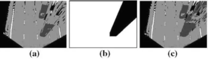
In the case in which there are vehicles in the scene, we use their prediction model, as we shall explain in Sect. 6, which defines the regions of the image that are more likely to con-tain vehicles in the next image via a binary mask. The prior information of each pixel for each class can be multiplied by the value of the corresponding pixels of the mask. Hence, the probability to belong to one of these classes of the pixels that belong to the black region of the mask (as shown in Fig. 1 lb), is set to a low value (typically 0.1, such that the prior for class vehicle is 0.9 for these pixels). As a result, the pixels of this
It can be obtained easily from the rectified images through the compu-tation of a simple translation plus rocompu-tation motion model, for instance, with point correspondences between consecutive images.
(a) (b) (c) Fig. 11 Prior probability map provided by vehicle tracking
black region will be more easily classified as belonging to the object class by the prior maps. Figure 11 shows in c and a, respectively, the segmentation results obtained with and without the use of this prediction model.
5 Road-plane element modeling
The information regarding lane markings and pavement given by the segmentation is used to estimate the presence and geometry of the lanes of the road. Our approach success-fully deals with challenging elements, such as curvature, an unknown number of lanes, lane changes, poorly painted lane markings, and lanes of variable width, as well as emerging and splitting lanes. The following sections describe the "lane tracker" technique that we use to detect and track the position of the ego-vehicle inside its own lane with time. Then, we discuss the estimation of the geometry of the lane that gives information about the curvature of the road, and finally, we investigate the presence of adjacent lanes, which is a feature that is not typically treated in the related literature.
5.1 Lane tracker
The lane tracker technique is commonly known as the func-tionality of an ADAS system that analyzes the evolution of the images and determines the width of the own lane, w*, and the position of the vehicle within it, x*. Hence, lane changes are also detected by analyzing the evolution of x* and w*.
This evolution is easily described as a dynamic linear sys-tem that can be solved with a Kalman filter defined by the following state-space equation:
x* = Ax*_, + Bu* n* (11)
where the state vector is x* = (x*, w*, x*, w*)T. The
mea-surement vector is, at each instant, z* = (x*, w*)T, which
is the instantaneous measurement of the target parameters. The following paragraphs explain how these measurements are extracted. The transition matrix, A, and the input control matrix, B, are given by a constant-velocity model. The use of this model does not mean that we assume a constant veloc-ity over all time; rather, the statistical model of the motion assumes undetermined accelerations with a Gaussian profile, modeled by n*.
Fig. 12 Image-plane to road plane transforms: Ho image-plane to road-plane; Hi image-plane to zoomed road-plane
The control matrix, B = (1, 0, 0, 0)T, is used to
mod-ify the estimation of the transversal position of the vehicle when lane changes are detected. The input control vector is obtained as u* if** > \(W ifx* < \{W Wk) Wk) (12) where W is the width of the image in pixels; hence, when the transversal position exceeds the boundary, at the left or right, of the estimated lane, the input control is activated and the transversal position is shifted.
The measurement vector, z*, is obtained by recomput-ing the transformed domain. Namely, a new zoomed road-plane image that contains information regarding a very near stretch of the road is created. Figure 12 shows the relation-ship between the image plane, the road plane, and this new zoomed road plane. As shown, the zoomed road plane con-tains only the very lower part of the original image plane in order to avoid the presence of vehicles. Within this zoomed image, only the lane markings that belong to the own lane are displayed and lane markings can be modeled by straight lines.
The measurement vector is obtained using the Hough transform on the segmented zoomed road plane. Two straight lines model the two lane markings of the own lane. These lines intersect the bottom boundary of the image in two points. The distance between these points is the measure-ment Wk, while the difference between their middle point and the mid-lower point of the image is x*.
The tracking process of the own vehicle position is depicted in Fig. 13. As shown, the noisy measurements are smoothed with the Kalman filter, which also allows the pre-diction and correct detection of the lane change event. 5.2 Lane modeling
In this section we discuss the process of modeling the own lane. This is done by selecting a set of control points of the lane along the transformed image and then fitting a pair of curves (one for each lane marking of the lane) using these control points.
****V/^
[Lane change t 3 left M e a s u r e m e n t s K a l m a n filtered
/
. . . . "
0 200 400 600 800 1000
k - Frame number
Fig. 13 Estimation of the transversal position of the own- vehicle inside its lane (varying from 100 to —100% corresponding to the left-most and right-most position inside the lane)
5.2.1 Control points generation
Given the segmentation of the image, in this stage we com-pute the control points, defined by their 2D positions, xlk,
which give enough information to model the geometry of the lane. The detection of the control points is carried out such that they are distributed throughout the whole image and constitute a quasi-regular grid, which is updated dynam-ically along time. This detection then allows for a better and easier estimation of the curve that best fits them.
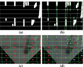
For each frame, the control points are updated as shown in Fig. 14, using their previously computed position and the set of new measurements obtained from the pixels that belong to lane markings. The measured control points are compared with the grid formed by the previous set of control points, depicted with circles in Fig 14c. These measurements are clustered around the previous control points, i.e., {xtk_l}i^l,
so that each previous control point has an associated set of M, measures, {z£;};=i> which are closer to it than to any other
control point. Therefore, the estimation of the control points depends on the number of measurements that fall inside its corresponding cell. The estimated value is computed as
' 4 - i ifM¿ = o
4=- 4 ^Mi = l (13)
z£* elsewhere
where z£* is the measure with the smaller distance to the previous control point:
Z^ = m i n { | | x [ _1- z ^ ' | | } (14)
5.2.2 Curve fitting
The complexity of the curve modeling of each lane marking increases as the number of control points being considered increases. The number of control points per lane marking, c, models different curve types. If c = 2, the model may be a line [25,26]; c = 3 defines generic second-order curves, such as parabolas [11,27], circles, and constrained cubic curves
(a) (b)
Fig. 14 Measurement generation: a blobs from dilated lane marking pixels; b intersection of Hough lines from each blob with horizontal lines; c previous image with its Voronoi cells division in solid lines, and the set of points xjj._j in circles; d current image with measured z'¿};
estimated z'¿ ; and predictions x'k_ j
approximating clothoids [12], while for c = 4, more com-plex spline shapes [13] can be estimated.
Typical approaches use parabolic models [11] for lane modeling, which offer enough accuracy for both transformed domain and original images. However, for the transformed images, generic circumference arc models show better per-formance in most situations.
Some researchers use the maximum likelihood method
[26,27] to estimate the parameters of these models. How-ever, RANSAC is preferred here as it is a robust estimation approach that shows much better performance by removing outliers from the set of points [22].
For better performance, we assume that the circumfer-ence center is at some point on the horizontal line defined by y = H, i.e., the bottom row of the image. This assumption forces the vertical to be tangent to the circumference in the lower part of the image, which is in line with the assumption that the vehicle is moving approximately parallel to the lane markings.
Figure 15 shows an example of curve fitting assuming a circumference model on the rectified domain. Note that the curvature is moderate in this type of motorways scenario such that the circumference model achieves a good trade-off between accuracy and simplicity.
5.3 Multiple lanes estimation
Once the own lane has been estimated in terms of position and geometry, the presence of adjacent lanes is hypothesized by assuming that these lanes have the same geometry and width, i.e., they are located at wk pixels at left and right.
(a) (b) (c)
Fig. 15 Curve fitting for an example image: a rectified image; b segmentation after Bayesian classifier; and c the resulting circum-ference model
Several adjacent lanes may be also hypothesized this way, considering a model defined by the parameter vector (xo, yo-, r ± n • Wkj1 where n indexes the number of hypothesized
lanes at left or right.
The verification of adjacent lanes is performed by check-ing the percentage of pavement pixels contained at each hypothesized lane. The probability that a hypothesized lane, indexed by I, actually exists is given by
ñ = ^ X p(-xp\**y) (15)
{xy}€l
where the summation is carried out only for the pixels within the hypothesized lane, whose cardinality is N. The same sta-tistic is computed for the "unknown" and "Lane marking" classes. Therefore, it is straightforward to determine the pres-ence of a lane if P¡ is greater than these statistics.
6 Vehicle detection and tracking
The strategy proposed for vehicle detection and tracking lies on the basis of a previous object segmentation in the trans-formed image. The proposed framework is flexible as it can operate over an arbitrary segmentation technique. Particu-larly, for this work the segmentation explained in Sect. 4 is used due to its efficiency and reliability. Based on this seg-mentation, the method achieves vehicle detection and track-ing by exploittrack-ing geometric and appearance information of the objects. It involves a collaborative analysis of the original and the transformed images. The former gives a complete view of the scenario ahead of the vehicle, but the information content is not homogeneously distributed among the pixels due to the perspective effect [28]. The latter, in turn, removes non-linearity at the expense of losing detail during the trans-formation.
First, vehicle detection is addressed by analyzing the segmentation image in the transformed domain. Vehicle can-didates are extracted using the geometric information of the objects in this domain (i.e., theeffect of thehomography over a volumetric object in the perspective image) and the
prop-erties of the bird's-eye view. On the other hand, the domain duality allows to verify the compliance of the measured can-didates with the expected appearance of vehicles in the orig-inal domain.
Additionally, vehicle tracking is obtained by associating the measurements at different instants, so that the track of each vehicle can be identified. The method comprises as well new vehicle management based on the spatial and temporal coherence of the measurements. Note that the transformed domain highly simplifies data association, as vehicles posi-tions and velocities are proportional to the corresponding actual magnitudes. Conversely, the original image allows to refine tracking results, both in the position and the dimension of the vehicles, which again supports the convenience of the proposed dual domain approach. Finally, coherent results in time are ensured by introducing the measurements in a prob-abilistic framework governed by a Kalman Alter. This frame-work enables us as well to make predictions of the vehicles positions in the following times. This is especially useful as it allows to maximize the information exchange between the segmentation process and the vehicle detection stage. Namely, a feedback loop is created in which the Bayesian segmentation framework receives theses predictions as prior probabilities.
6.1 Measurement generation
As stated, measurements for vehicle detection are extracted from the dual domain analysis based on the segmentation explained in Sect. 4. The regions of the image segmented as objects are taken into account at this stage. Note that all vehi-cles contain a dark area in their lower part due to shadow and wheels, which will be classified as object. This dark part is enlarged in the transformed domain, as shown for the white vehicle in Fig. 8b). However, this segmentation is performed at a pixel level; hence, the result often shows unconnected regions and is corrupted by noise (see Fig. 16b, where the pixels belonging to the object class are painted in white). Therefore, a morphological opening operation, i.e., an ero-sion followed by a dilation, is performed to obtain enhanced images in which objects are clearly segmented. The initial erosion (typically involving a small square structuring ele-ment) removes background noise, whereas the subsequent complementary dilation operation restores the contours of the objects, as shown in Fig. 16c, d, respectively.
As a result of these operations, an enhanced image is obtained, which consists of several compact white zones (known as blobs). These blobs, characterized by their posi-tion, x, and width, w, as illustrated in Fig. 16e, represent the hypotheses for the vehicles in the image. The verifica-tion of these hypotheses is performed twofold. First, the nature of the underlying projectivity to the road-plane is taken into account. Namely, the homography produces a
Fig. 16 Image in b shows the segmentation of a.
c, d Correspond to the erosion of b and dilation of c, respectively. A typical blob is shown in e, where only the lower part is taken into account
due to perspective distortion
1
"N . . . •%
1
(a) (b) (c)
radial distortion of the elements of the objects above the road plane, as can be observed in Fig. 2. Hence, only the candi-dates showing a shape compliant with this kind of distortion are considered. Observe that in the example in Fig. 16d both candidates have the expected shape.
On the other hand, the dual domain approach allows to check the appearance of the hypothesized vehicles in the original domain. The inverse homography H_ 1 delivers the
position and width of the candidates in this domain. Addi-tionally, assuming a standard aspect ratio of vehicles (i.e.,
1.2:1) a rectangular region is defined around each hypothe-sized vehicle position. The verification is performed in these regions, and is based on different cues for close and distant objects. For the former, a symmetry measure is used, since the rears of vehicles have a high degree of symmetry around the vertical axis. Hence, the vertical symmetry, denoted / and normalized between 0 and 1, is computed as in [17] inside the bounding box. Regions with high symmetry values ( / > i/) are classified as potential vehicles. As for distant vehicles, the resolution is usually not sufficient to provide a signifi-cant symmetry value. In this case, the edge density is used as a cue for vehicle verification. Vehicles present a high density of edges owing to their contrast with the background, plate, back glass, etc. Hence, the edge density is computed in the hypothesized window as
d 1
RxRy
X
e(
x>y">
(16)x,ynR
where e(x, y) is the edge intensity of pixel (x, y) between 0 and 1 computed using the Sobel edge detector, and R is the bounding box of the candidate, with dimensions Rx x Ry.
Candidates with high edge density values (d > to) are classified as potential vehicles. The thresholds tf and t¿ are defined in such a way that the negative classification of true
vehicles is minimized, even if it involves some false detec-tion. These can be effectively filtered in the tracking stage due to their lack of coherence and persistence, as explained below.
6.2 Vehicle tracking
The segmentation provides instantaneous measurements of the positions of the vehicles. However, valuable insight in the characterization of the vehicles (position, trajectory, new vehicle entries, etc.) can be attained by analyzing the tempo-ral evolution of these measurements. Remarkably, the trans-formed domain constitutes a suitable framework to perform temporal correlation: in effect, it provides an up-to-scale reconstruction of the road plane and thus data association can be performed on the basis of Euclidean distances. This largely simplifies as well vehicle entry and exit management. Additionally, in the transformed domain motion of vehicles is proportional to their true motion; thus it can be modeled via a linear process based on Kalman filtering. On the other hand, the lack of accuracy and of height information inherent to this domain are compensated by resorting to the original domain, which is richer in details and hence provide refined data.
6.2.1 Data association
Note that at each instant independent results are obtained for the set of vehicles. In addition, occasionally some false pos-itives or negatives can occur as a result of poor segmentation of the objects. Therefore, data association between frames is needed. The objective is to assign n measures in the cur-rent frame to m existing vehicles. In this work, a clustering technique based on a similarity criterion is applied. Namely, a similarity function is defined that compares the attributes
i
(a) ( b )
Fig. 17 Examples of the applied clustering technique. Predicted vehi-cles are painted with a solid line and a cross in the middle (the cross indicates position x^,, and the segment corresponds to width wp), and
blobs associated with them are patined as isolated crosses
fc + 1 k + 2 fc + 3
Fig. 18 New object management. At time k, a new blob appears in the image, which already contains one existing vehicle. The new blob fulfills both spatial and temporal coherence criteria at times k + \, k + 2 and k + 3; thus, it is classified as a vehicle and tracked henceforth
of each current candidate, (xc, wc), with those predicted for
each vehicle, (xp, wp). The similarity is modeled as a
func-tion of two factors relating to the relative posifunc-tion and the relative width of the candidates as
S- Wr 1 (17)
The distance is defined as a Euclidean metric, and it consid-ers the mid-lower pixel of the blob as defined in Fig. 16e.
Naturally, the blob that maximizes the similarity function for each vehicle is assigned to it. Clustering is illustrated in Fig. 17 with two examples, in which the predictions are shown with line segments with a cross in the middle, and the attributes of the candidates most similar to them are painted as isolated crosses. In Fig. 17a, five blobs are segmented and only three vehicles are predicted; the assignment is clear as the position and width of the selected blobs are very similar to the predictions. In Fig. 17b, three blobs are found for two predicted vehicles. Here, for the lower predicted vehicle, the larger blob is selected although the small blob in the left is slightly closer to the prediction, due to its similarity in the width. Finally, if no measurement is found for the vehicle, the tracking process relies on the predicted attributes associated with it. This reveals the suitability of the predictive nature of the proposed framework.
6.2.2 New vehicle management
The above method relates existing vehicles with their cor-responding new measurements. However, new vehicles may enter the scene at time k. These appear as additional blobs in the enhanced segmentation image. On the other hand, some spurious blobs may also arise due to artifacts in the segmen-tation. A twofold verification (i.e. spatial and temporal) is carried out to differentiate the blobs corresponding to enter-ing vehicles. First, due to kinetic constraints between con-secutive frames, vehicles may only appear in the uppermost (far vehicles coming closer) or lowermost (vehicles overtak-ing the own vehicle) zones of the road-plane image. Hence, to ensure spatial coherence, only these zones are analyzed.
Additionally, a temporal coherence criterion is enforced for the remaining blobs, i.e., a set of similar blobs is sought in the following frames (see Fig. 18). The similarity function is evaluated for every set according to the descriptor in (17).
Eventually, a new vehicle is hypothesized when the elements ofthe set fulfill the similarity condition S > 2/t¿. Visually, this condition holds if, after the initial observation of the blob at time k, a blob is found at subsequent time points that is inside the search area of radius ta (||x^ — xc || < to) and has
a width at maximum of 50% larger or smaller than the initial .\wp-wc\
observation (] 1/2). This is the case for the example
in Fig. 18, where the position and width ofthe detected new blob are similar throughout four consecutive frames. Note that both the spatial and the temporal verification are widely simplified due to operation in the homogeneous transformed domain, as opposed to classical approaches working in the original domain, which usually require more complex anal-ysis or additional a priori conditions.
6.2.3 Detection refinement
Results obtained in the transformed domain provide a coarse approximation to ground truth, as the change of domain entails a certain loss of accuracy. In addition, the transformed domain involves a bird's-eye view and thus removes infor-mation regarding the height dimension of the vehicles. The proposed collaborative approach is exploited here to shift the processing to the original domain. The objective is two-fold: (i) to refine the widths and positions obtained in the transformed domain, and (ii) to allow the estimation of the height of the vehicles in order to provide a more complete characterization.
Refinement in the original image is based on edge informa-tion; in effect, the contour ofthe vehicle rear usually presents abrupt edges. Hence, edge information is used to refine the bounding box of each vehicle. The rectangle bounding the vehicle is obtained using the inverse homography H_ 1 in
the same manner as in Sect. 6.1. In order to ensure that edges are contained in it, the region is expanded around the hypoth-esized bounding box, and the Sobel edge detector is applied
(c)
Fig. 19 Vehicle detection refinement: a A detail of the closer vehicle in c; b is the result of Sobel operator over a. Observe that both the ver-tical and the horizontal edge histograms feature prominent peaks in the positions of the vehicle contour
over all of the pixels in the extended region. This is illustrated in Fig. 19: the image in b corresponds to the edge intensi-ties computed over the image in a, which in turn shows a detail of the closest vehicle in c. Then, the resultant edge sub-image in b is scanned and the values are added up, first left to right to produce the horizontal edge histogram, and, in turn, bottom to up to render the vertical edge histogram (see Fig. 19b). The former is expected to have prominent peaks for the upper and lower limits of the vehicle, while the second will contain two peaks, for its left and right lim-its. The local maxima are selected at each side of the his-togram so that a refined bounding that fits the real contour of the vehicle box is finally obtained. The achieved fine-tuning is illustrated in Fig. 19c, where the solid line depicts the coarse detection obtained from the transformed domain, and the dotted line corresponds to the refined bounding box. As a result of this stage, height information is added to the previous vehicle attributes, position and width, which are in turn fine-tuned.
6.2.4 Probabilistic filtering
So far, the method obtains sequential measurements for each of the vehicles in the scene. These measurements are time-correlated (i.e., a track is kept for each vehicle) but lack coherence in what concerns their fitting the known dynamics of vehicles. In effect, vehicles move forward with a locally uniform pace, especially in highways. Therefore, smooth changes are expected in the position of the vehicles on the road and their velocity is approximately constant, at least locally. This knowledge allows to introduce the measure-ments into a probabilistic framework that filters noisy instantaneous measurements, thus providing smooth results. In particular, in the transformed domain vehicle dynamics are
proportional to their actual magnitudes; hence the state evolu-tion in this domain can be considered to be linear. Therefore, the transformed domain enables us to model vehicle kinetics with a constant-velocity Kalman filter.
The state vector is composed of the position (x, y), velocity (i, y), width (w), and normalized height (h) of an object:
xjt = (x, y, x, y, w, h)T (18)
For every time point k, the object attributes (position, width and height) are measured; thus, the measurement vector zk
is given by
zk = (x, y, w, h)T (19)
Both the position and width measurements refer to the road-plane image, where the linearity condition holds. Hence, these measurements must be transformed back to the origi-nal image after the refinement stage. Conversely, the height information only exists in the original image, where it is non-linear due to perspective. To make it non-linear, a normalized height measure, h, is defined as in [29].
As regards the choice of the process and measurement noise covariance, the following considerations are insight-ful. First, the process noise must be low due to the adequacy of the linear evolution of the state vector for a real scenario. In particular, the noise covariances of the width and height attributes are almost zero, as the dimensions of the object are actually constant. As for the measurement noise, the uncer-tainty is larger as it depends on the accuracy of the segmen-tation. In any case, its covariance should be larger that of the process noise in order to prevent the system from being corrupted by poor measurements. Noise covariances may be tuned to adapt more quickly to changes in the measurements or to enforce smoothness, as long as the process noise remains smaller than the measurement noise.
Note that the predictive nature of the Kalman filter is of great value as it allows to create a feedback loop which enriches other stages of the system. Indeed, predictions are used to perform data association on the incoming measure-ments (see Sect. 6.2.1). Moreover, they are also used to feed back the segmentation process, namely the expected posi-tions of the vehicles are used to define the prior probability to belong to the object class. In effect, since the vehicle posi-tion and width estimates are available, and given the radial distortion produced by the road plane homography, it is pos-sible to infer the regions potentially containing objects in the following frame. In this work, a binary probability map is generated as shown in Fig. 1 lb. This feedback loop allows to maximize data exchange between modules and thus to capitalize on all available information.
7 Tests and discussion
All the developments have been carried out in C++ program-ming language, under an MFC solution for Windows and Direct Show primitives. This architecture allows for a real-time performance of the system for real on-road operation as well as continuous visualization of the processed data. More-over, the system was designed to be able to acquire the video stream from different digital interfaces, such as USB, Fire-Wire, GEthernet, etc. Nevertheless, for the trials, the acquir-ing system was composed of a forward lookacquir-ing digital video camera SONY HDR-HCR5E, installed near the rear mirror, and a FireWire connection to the processing system. The size of the images is 360 x 288, which allows the system to work near real-time, at 15 frames per second on average (including video visualization and output data generation) in a laptop Core2Duo at 2.2 GHz with 2 GB of RAM.
The real on-road trials have been conducted in differ-ent roads in Madrid, Brussels, Milano, Torino, and the A4 Brescia-Padova motorway (during the test sessions carried out in different stages of the I-WAY integration activities). From these trials, we have collected a large number of sequences (with a total length of around 150 min) from which we have gathered relevant output data. The target is to analyze the behavior and the performance of the system, monitoring its main output parameters, namely, the position of the vehi-cle inside its lane, the number of lane changes, the curvature, the positions of the vehicles ahead, and their dimensions.
Different scenarios are considered to demonstrate the abil-ity of the system to adapt to the uncontrolled outdoor sce-nario, including changing illumination conditions, different pavement color, varied weather conditions, different type of lane markings, presence of vehicles that cause occlusions, etc. Attending to the results obtained through the tests, we can extract the following conclusions:
The position of the own vehicle inside its lane (a feature that depends on the lane tracker performance, described in Sect. 5.1) is estimated with high accuracy in almost all situa-tions. Some examples are shown in Fig. 20. The central over-laid region defines the closer part of the own lane, according to the detected lane markings, depicted with thick solid lines. The center of the lane is marked with a thin solid line, and the center of the image with a shorter black line. The relative position of the vehicle in the lane is depicted with a numerical indicator, which is 0% at the center of the lane, and -100 and 100% at its left-most and right-most position, respectively. As shown, the width of the lane may vary, but it is accurately estimated by the system.
The lane change detection is one of the higher perfor-mance features of the developed system (as will be shown in Table 1). The second row of Fig. 20 shows some detected lane changes, whose direction is indicated with a superimposed icon. The detection of the significant curves depends on the
visibility of the lane markings in the far distance, which is generally good provided that the traffic load is not too heavy. In these situations, the system correctly detects the curvature, as in the examples shown in the third row of Fig. 20.
Regarding the detection of multiple lanes, the system has shown excellent performance in most situations. As long as the segmentation result is correct, which is true for most situ-ations, the system is able to hypothesize the presence of adja-cent lanes to the own lane and confirm their presence using the Bayesian segmentation information. Different examples illustrate this ability in the Fig. 20: when driving in the right lane, the system is able to determine that there are no more lanes at the right, and analogously when driving in the left-most lane. When driving in the central lanes, three lanes are hypothesized at most. This number is not a limitation of the algorithm, but a design parameter, as beyond these there are not enough pixels to take a reliable decision.
In the field of vehicles detection, most of the cars are cor-rectly detected in the region of interest (up to 35 m inside the detected lanes) for all the considered scenarios. The Fig. 20
shows several examples of detected vehicles, represented by a rectangular box around these, that illustrate the dimensions of the vehicles, as well as their location inside the lanes. Provided that the camera is calibrated, its distance in meters to the camera is printed with a yellow numerical indicator. First, recall that the dimensions of the vehicles are typically well estimated, up to some errors due to the presence of intense edges at the background. Second, the tracking frame-work allows to keep track of the vehicles, giving a temporal coherence to the detection, as well as robustness against brief occlusions, such as the one shown in the two last images of Fig. 20. This is a raining scene, where even with the presence of the wipers, which appear and occlude the vehicle momen-tarily, the tracker succeeds in maintaining the detection of the vehicle for successive frames.
One of the major abilities of the proposed system is its demonstrated robustness against challenging, unpredictable situations. On-road trials feature, for instance, sudden illumi-nation changes (e.g. when entering into tunnels, or passing below a bridge), the appearance of the aforementioned ele-ments such as wipers, drawings on the road, drops on the windscreen, irregular color of the pavement, reflections, etc. The proposed models rely on the robustness of the probabi-listic segmentation, that is able to handle any of these diffi-culties with the "unknown" class. In few words, the system has been designed to search for and model lane markings, the color of the pavement and vehicles, and to not be deceived by this type of uncontrolled scenarios.
Figure 20 show the excellent performance of the sys-tem for a wide variety of scenarios. In order to reflect more objectively the performance, a set of relevant parameters has been defined, i.e., vehicle detection rate (VDR), lane change detection rate (LCDR), vehicle false positive rate (VFPR),
Fig. 20 Examples showing the detected elements of the road: In the upper row some representative examples of the accuracy of the lane tracker are shown; the second row shows examples of lane change events; and the lower row illustrates vehicle detected in difficult scenarios
Table 1 Detection results for different scenarios Event
No. of total vehicles No. of detected vehicles No. of lane changes No. of detected lane changes No. of false positive vehicles No. of false positive lane changes VDR (%) LCDR(%) VFPR (%) LCFPR (%) Type of Typical 1,056 1,021 204 196 21 3 96.69 96.08 1.98 1.47 scenario Complex 1,177 1,079 211 197 46 9 91.67 93.36 3.90 4.27
and lane change false positive rate (LCFPR). The former two are defined as the number of correct detections over the total number of events (presence of vehicle or lane change,
respectively) indicated by the ground truth. The latter are defined analogously as the number of false positives. They have been measured off-line for a large set of sequences corresponding to two scenarios: typical and complex. The former involves the typical driving conditions in motorways, that is, well-painted lane markings, variable illumination con-ditions with soft changes, low/medium traffic density, or favorable weather conditions (including mild rain). The latter comprises those conditions that are not so commonly encoun-tered in motorways (such as dense traffic or variable illumi-nation conditions with rapid and abrupt variations), or those that occur for short periods of time (such as tunnels, which entail artificial illumination conditions).
Table 1 shows the performance of the system, in terms of detection and false positive rates, for the two sets of scenar-ios. As can be observed, the vehicle detection and the lane change detection rates are very high (over 96%) in a typi-cal scenario. In this situation, the false positive rate is under 2% for both features. As for complex scenarios, the vehicle