Hyperspectral imaging for predicting soluble solid content of starfruit

(1)

73:1 (2015) 83–87 | www.jurnalteknologi.utm.my | eISSN 2180–3722 |

Full paper

Jurnal

Teknologi

Hyperspectral Imaging for Predicting Soluble Solid Content of Starfruit

Feri Candra , Syed Abd. Rahman Syed Abu Bakar*

Computer Vision, Video and Image Processing Research Lab,Electronics & Computer Engineering Department, Faculty of Electrical Engineering, Universiti Teknologi Malaysia, 81310 UTM Johor Bahru, Johor Malaysia

*Corresponding author: [email protected]

Article history

Received: 9 September 2014 Received in revised form: 2 November 2014 Accepted: 1 February 2015

Graphical abstract

Abstract

Hyperspectral imaging technology is a powerful tool for non-destructive quality assessment of fruits. The objective of this research was to develop novel calibration model based on hyperspectral imaging to estimate soluble solid content (SSC) of starfruits. A hyperspectral imaging system, which consists of a near infrared camera, a spectrograph V10, a halogen lighting and a conveyor belt system, was used in this study to acquire hyperspectral images of the samples in visible and near infrared (500-1000 nm) regions. Partial least square (PLS) was used to build the model and to find the optimal wavelength. Two different masks were applied for obtaining the spectral data. The optimal wavelengths were evaluated using multi linear regression (MLR). The coefficient of determination (R2_{) for validation using the model}

with first mask (M1) and second mask (M2) were 0.82 and 0.80, respectively.

Keywords: Hyperspectral Imaging; Partial Least Square Regression; Starfruit

1.0 INTRODUCTION

Starfruit is one of Malaysia’s main exported fruits. Since 1989, Malaysia has been the largest exporter of starfruit in the world. In 2008, 3648.9 metric tons of starfruit were exported to various countries in Europe (the Netherlands, France, Germany), Middle East (Saudi Arabia, Iran, Bahrain, Turkey), and Asia (Singapore, Hongkong, Indonesia). Until June 2009, the export record shows that a total of 901.509 metric tons of starfruits had been exported [1].

In Malaysia, numerous studies have been carried out to enhance the postharvest handling of starfruit to increase the consumer acceptance and satisfaction. In spectroscopy area, recently, Omar et al. [2][3] conducted a study on nondestructive intrisic quality measurement of starfruit such as pH, firmnes dan soluble solid content of starfruit using spectrocopy method. In image processing field, Abdullah et al.[4] had developed an automated quality inspection of starfruit based on the colour of starfruit. Mokji [5] had developed an algorithm with 2-dimensional colour maps to classify starfruits into six maturity grades. Meanwhile, Amirulah et al. [1] implemented Mokji’s algorithm on Field Programmable Gates Array (FPGA). Other reseachers [4][6] have also studied defect detection of starfruit. In recent years, hyperspectral imaging (also called imaging spectroscopy) has become a popular tool for quality and safety inspection of food and agricultural products [7]. Hyperpectral

imaging combines spectroscopy and imaging techniques to obtain both spatial and spectral information of an object. The hyperspectral technique can be used for inspecting defects in fruit, predicting constituents of fruit to estimate its quality, food quality evaluation and sorting fruits. In addition, this technique can be applied to measure some internal attibutes of fruit simultaneously and non-destructively [8].

A number of studies have been reported on the application of hyperspectral imaging technique to evaluate quality of various fruits.This technique has been successfully used for detecting defects in various fruits such as apple [9], citrus [10], and cucumber [11][12]. For determining quality attribute measurement of fruits such as soluble solid content (SSC) and firmness, reseachers have conducted studies on a number of fruits such as apple [13][14][15], strawberry [16], bluberry [17], banana [18], grapes [19], pickles [11], and tart cherries [20]. These studies have shown the potential of hyperspectral imaging for fruit quality inspection using spatial dan spectral information. However, due to its non-circular shape, no study has been reported on using hyperspectral imaging for starfruit quality inspection. Hence, in this work, two types of region of interest (ROI) are introduced for the inspection.

The main objective of this study is to investigate the potential of hyperspectral imaging for estimating the soluble solid content of starfruit. The specific objectives are (1) to use hyperspectral imaging system to acquire the hyperspectral image

(2)

of starfruit in region between 500 and 1000 nm, (2) to identify several significant wavelengths that can be utilized for predicting soluble solid content of starfruit, (3) to evaluate the use of different area measurement (region of interest) to obtain the spectral data, and (4) to develop a novel calibration model using the optimal wavelengths.

2.0 MATERIALS AND METHODS

2.1 Starfruit Samples

A total of 72 samples were obtained from a starfruit farm. The samples were selected in such a way that each grade of samples could be represented by the same number. This study applied maturity standard set by FAMA (Federal Agricultural and Marketing Authority), Malaysia, with six indeces. Lower index (index 1 and 2) would indicate that the starfruit is verdant while higher index (index 5 and 6) would indicate mature fruit. The samples were scanned in hyperspectral imaging system using image acquistion for determining the soluble solid content (SSC) of samples.

2.2 Hyperspectral Imaging System

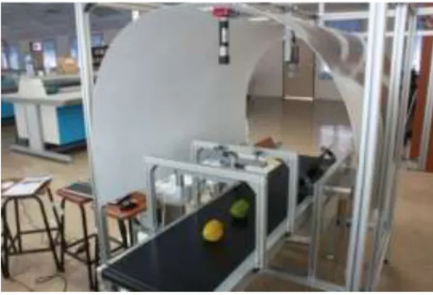
A hyperspectral imaging system (Figure 1) developed in the computer vision, video and image processing (CVVIP) laboratory, Faculty of Electrical Engineering, Universiti Teknologi Malaysia, was used for this experiment. The imaging unit consisted of a 12-bit digital NIR camera and a spectrograph. A MVI 1312 Photonfocus camera was used. A V10 (Spectral Imaging Ltd, Oulu, Finland) spectrograph was attached to the camera to acquire hyperspectral images. An illumination unit, which consisted of two 150 W halogen lights powered by a DC voltage regulated power supply (Line light QDF5072 and DC950H, Dollan Jenner Industries, Inc, USA) was positioned at angle of 450 _{to illuminate}

the camera’s field of view. A conveyor unit with adjustable speed was used to move and present the starfruit for imaging. Futhermore,a computer with a frame graber (National Instument) was used for acquiring and processing the hyperspectral images. MATLAB software was used to create a program for image acquisiton and analysis. The size of hyperspectral image generated by this system was 460X360 pixels with 180 spectral bands (wavelengths) from 500 to 1000 nm.

Figure 1 Hyperspectral imaging system

Before acquiring the hyperspectral image, spectral and reflectance calibration were carried out to ensure accuracy in the measurement. The purpose of spectral calibration was to assign a discrete wavelength to the hyperspectral image band [8]. This calibration was accomplished by using a spectral calibration lamp, Hg(Ar) (Oriel Model 6035, Oriel Instruments, Stratford, CT,

USA). Next, reflectance calibration was also perfomed using a white reference with standard reference of 99% (Teflon) to compensate the non-linear sensitivity of the camera.

2.3 Collecting Spectral Data

Due to the complex shape and uneven surface of starfuit, two approaches were used for collecting the spectral data of each starfruit. The first method, M1, was used to utilize the whole starfruit area as measurement area or region of interest (ROI). The second method, M2 was used to designate only some portion of starfruit area as ROI. The binary masks were created using both methods. Then, the masks were used for calculating the relative reflectance average of ROI of each sarfruit in wavelength range between 500 and 1000 nm.

(a) (b)

Figure 2 (a) a starfruit image at 733.2 nm; (b) the mask M1

Using the first method (M1), image at 733.2 nm (Figure 2a) was selected for building the mask. The image gave the maximum contrast between the starfruit and the background. Therefore, the starfuit and the background could be segmented easily by simple thresholding. Also, the image at that wavelength was smoothened using an averaging filter to remove the noise. Then, the smoothened image was segmented by using Otsu’s method [21]. Finally, the morphological operations, such as dilation and erosion, were applied to improve the quality of the image. The mask generated by this method (M1) is shown in Figure 2b. Mask M1 was then used for creating mask M2. Centre of mass (centroid) and bouding box value of white area in Figure 3a was computed using Matlab. Accordingly, two rectangles, r1, and r2, were build. The size of the rectangles were determined such that the position of the rectangles must be in the middle on the left and right side of starfruit. Figure 3b shows mask for M2. Mask M1 and M2 were used for obtaining the spectral data of each sample. Then, the performance of each the masks was evaluated.

(a) (b)

Figure 3 (a) Mask M1 was used to determine the bounding box and cetroir value; (b) Mask M2

(3)

2.4 Reference Measurement

After acquiring the spectral images, measurement of soluble solid content (SSC) of samples was carried out destructively. The samples were crushed using a juice extractor. Then, the juice of each samples was measured for its soluble solid content (SSC) using a digital hand-held pocket refractometer (PAL-α, Atago Co., Ltd., Japan). The SSC values were then used as references for developing the calibration model.

2.5 Building The Calibration Model

Partial least square regression (PLSR) was used to build the calibration or prediction model. This regression is a technique that generalizes and combines all features from principal component analysis and multiple regression. Its aim is to predict or analize a set of dependent variables from a set of independent variables or predictors. In this study, PLSR was developed to find the mathematical relationship between the spectra response and one attribute of starfruit (soluble solid content).

The predicted value of the attribute of interest 𝑌̂ was determined as follows[16]

𝑌̂ = 𝑋𝑊𝑎𝛽 = 𝑇𝑎𝛽 (1)

𝑊∗_{= (𝑊(𝑃}′_𝑊)−1₎₍₂₎

where 𝑎 is the number of PLS components, P’_{is the wavelength}

loadings and β is the regression coefficient.

The number of PLS components is determined by the complexity of the model. The complexity increases with the increase of the number of PLS components. In this study, the optimum complexity of the model was estimated by using k-fold cross validation.The sample set was randomly split into k segments. One segment was left out as a validation set. The others (k-1 segments) were used as a training set. This procedure was repeated k times so that each segment would all be used as validation set in turn. In this experiment, k was set to 10. The result was a residual matrix. The mean squred error for validation (MSECV) was calculated from the residual matrix.

𝑀𝑆𝐸𝐶𝑉=1_𝑛∑𝑛𝑖=1(𝑦𝑖− 𝑦̂𝑖 𝐶𝑉)2 (3)

where 𝑦𝑖 and 𝑦̂𝑖 𝐶𝑉 are the measured and predicted values of

attribute, while n is the number of sample.

The local minimum approach [22] of MSECV was used for

determining the optimum number of PLS component. This approach is used to avoid overfitting. Afterwards, feature (variable) selection was done by using PLS-BETA method [23][24]. The method applies regression coefficient (β) to identify the most influential wavelength. The wavelength that has the highest absolute value was considered as the optimal wavelength. Otherwise, the wavelengh that has the lowest is negleted because it would only contribute little to the model.

Only selected optimal wavelengths were used to build the multi linear regression (MLR) models instead of using the whole wavelengths. The formula of MLR is as follows [18]

𝑌̂ = 𝑎0+ ∑𝑁𝑁=1𝑎𝑁𝑅𝜆𝑁 (4)

where 𝑌̂ is the predicted value of the attibute; N is the number of optimal component; 𝑎0 and 𝑎𝑁 are the regression coefficients and

𝑅𝜆𝑁 is the reflectance intensity at a wavelength.

The performance of the calibration model was evaluated using MSE and the coeficient of determination (R2_{), expressing}

the proportion of variance explained by the model. The formula is defined as follows[17]

𝑅2_{= 1 −}𝑅𝑆𝑆

𝑇𝑆𝑆 (5)

where 𝑇𝑆𝑆 (Total sum of squares) = ∑𝑛𝑖=1(𝑦𝑖− 𝑦̅)2,

𝑅𝑆𝑆(Residual of squres) is ∑𝑛𝑖=1(𝑦𝑖− 𝑦̂)𝑖 2, 𝑦̂𝑖 is the predicted

value, while 𝑦𝑖 is measurement value.

3.0 RESULTS AND DISCUSSION

3.1 Reflectance Spectra

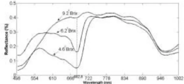
Figure 4 and 5 show the reflectance spectra of three starfruits with different SSC values (o_{Brix) using mask M1 and M2, respectively.}

The curve using mask M1 had the same shape as M2 in whole wavelength range. However, both curves had different reflectance value, especially in range between 708 nm and 1002 nm. The reflectance value of the samples increased when the SSC value was increased in wavelength between 590.4 nm and 1002 nm for M1, and between 621.2 nm and 708 nm for M2. Both figures show that reflectance value had significant change at 682.8 nm for M1 and M2. At this wavelength, a strong absorbance was observed clearly, which was due to the change of the chlorophyll pigment. Lower SSC value had stronger absorbance, meaning that the chlorophyll pigment of starfruit was high. As a result, the reflectance value decreased. In contrast, the high reflectance value or high SSC value had lower absorbance and chlorophyll pigment. The high reflectrance showed high maturity grade of starfruit. This wavelength (682.8 nm), which had sensitivity to chlorophyll change, was similiar to the wavelength as reported by previous reseachers [16][18].

Figure 4 Reflectance spectra of three samples with different SSC values using mask M1

Figure 5 Reflectance spectra of three samples with different SSC values using mask M2

3.2 Optimal Wavelength Selection

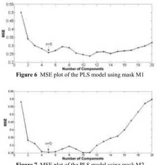
Two PLS calibration models were build using the whole spectral range consisting of 180 wavelengths. The first model was established using mask M1, while the second model was created using mask M2 as ROI. To find the optimal wavelength for each model, the same procedure was applied to both models. Before optimal wavelengths selection was done, the optimum number for each of the model was determined using the local minimum approach based on MSE value. Figure 6 and 7 show the plot of MSE versus PLS components for M1 model and M2 model,

(4)

respectively. Although using different ROIs, both models had a similar local minimum at n = 5.

Figure 6 MSE plot of the PLS model using mask M1

Figure 7 MSE plot of the PLS model using mask M2

Figure 8 and 9 show the regression coefficient (β) plot versus the wavelength of both models using the optimal component (n = 5). The PLS-BETA method was used to find the significant wavelengths. By using Matlab, the maxima and minima of β values for both models were selected. The optimal wavelengths for M1 model were 565.2, 657.6, 702.4, 741.6, 859.2 and 943.2 nm (six wavelengths), respectively. Meanwhile, the optimal wavelengths for M2 model were 565.2, 677.2, 736, 873.2 and 943.2 nm (five wavelengths), respectively. The results showed that M2 model had lesser amount of wavelengths than M1 model despite having the same number of PLS components.

Figure 8 Regression coefficient plot of M1 model with n=5

Figure 9 Regression coefficient plot of M2 model with n=5

3.3 The Performance Of The Model Using The Optimal Wavelengths

The optimal wavelengths, which were selected using PLS, were evaluated using multi linear regression (MLR) for predicting the

SSC value of starfruit. Table 1 shows the performance of the models built by using MLR and the optimal wavelengths. The performance was evaluated via cross validation (CV). Figure 10 and 11 show the plot of the predicted and measured SSC values for calibration and validation. In general, the model created using mask M1 had better performance than the model created using M2, although the performance of both models had small differences. For MSE value, the M1 model was lower than the M2 model for calibration and validation. Meanwhile the R2_{of M1}

model was higher than that of the M2 model. However, M2 model had smaller number of wavelengths than M1. Both models have shown good performance because R2_{values are high (0.82 and}

0.80 out of scale of 1). The following equations were derived based (2); 𝑦̂ = 7.06 − 4.63𝑅(565.2)− 3.43𝑅(657.6)+ 17.62𝑅(702.4) − 23.51𝑅(741.6)+ 12.86𝑅(859.2)+ 3.81𝑅(943.2) (6) 𝑦̂ = 7.40 − 0.77𝑅(565.2)+ 9,01𝑅(677.2)− 17.35𝑅(736) + 12.722𝑅(873.2)− 2.07𝑅(943.2) (7) where 𝑦̂ is the predicted SSC value; R(λ)is the reflectance intensity

at λ. Equation (6) was used for estimating the SSC value using mask M1. Meanwhile, (7) was used for estimating the SSC value using mask M2. These equations can be used for multispectral application. For simpler application, the model with mask M2 and five wavelengths could be considered for predicting the SSC value of starfruit non-destructively.

Table 1 The performance of the model using MLR and the optimal wavelength

ROI Wavelength (nm)

MSECal MSEVal R2Cal R2Val M1 565.2, 657.6, 702.4, 741.6, 859.2 and 943.2 0.228 0.274 0.85 0.82 M2 565.2, 677.2, 736, 873.2 and 943.2 0.259 0.305 0.83 0.80

Figure 10 The predicted and measured SSC values of the model created using MLR, mask M1 and optimal wavelengths

(5)

Figure 11 The predicted and measured SSC values of the model created using MLR, mask M2 and optimal wavelengths

4.0 CONCLUSION

In this study, a hyperspectral imaging system was used to acquire hyperspectral images of starfruit. This system was successfully applied to predict the soluble solid content (SSC) of starfruit. The models were built using different ROI, and the optimal wavelengths were evaluated. The model created using mask M1 showed better performance. For simpler application, the model created using mask M2 could be considered for estimating the SSC value of starfruit.

Acknowledgement

The authors would like to express gratitude for the financial support received from the Ministry of Science and Technology Innovation (MOSTI) Malaysia under VOT: 79366.

References

[1] R. Amirulah, M.M. Mokji, and Z. Ibrahim. 2010. Implementation of starfruit maturity classification algorithm on embedded system. 2010 2nd International Conference on Signal Processing Systems. 1: 810–814.

.http://dx.doi.org/10.1109/ICSPS.2010.5555248

[2] A.F. Omar and M.Z. Matjafri. 2013. Specialized Optical Fiber Sensor for Nondestructive Intrinsic Quality Measurement of Averrhoa Carambola.

Photonic Sensors. 3(3): 272–282. http://dx.doi.org/ 10.1007/s13320-013-0111-x

[3] M.Z. Abdullah, J. Mohamad-Saleh, A.S. Fathinul-Syahir, and B.M.N. Mohd-Azemi. 2006. Discrimination and classification of fresh-cut starfruits (Averrhoa carambola L.) using automated machine vision

system. J. Food Eng. 76(4): 506–523.

http://dx.doi.org/10.1016/j.jfoodeng.2005.05.053

[4] M. Mokji, S.A.R. Abu-Bakar. 2006. Starfruit Grading Based on 2-Dimensional Color Map. Regional Conference on Engineering and

Science (RPCES). 203–206.

http://eprints.utm.my/1691/1/musa2006_Starfruit_grading.pdf

[5] M.F.A. Kamil, M. Mokji, U.U. Sheikh, and S.A.R. Abu-Bakar. 2010. Machine Vision for Starfruit (Averrhua Carambola) Inspection. 2010

Fourth Asia Int. Conf. Math. Model. Comput. Simul. 333–336.

http://dx.doi.org/10.1109/AMS.2010.73

[6] A.A. Gowen, C. Odonnell, P. Cullen, G. Downey, and J. Frias. 2007. Hyperspectral imaging – an emerging process analytical tool for food

quality and safety control. Trends Food Sci. Technol. 18(12): 590–598.

http://dx.doi.org/10.1016/j.tifs.2007.06.001

[7] J. Qin, K. Chao, M.S. Kim, R. Lu, and T.F. Burks. 2013. Hyperspectral and multispectral imaging for evaluating food safety and quality. J. Food Eng. 118(2): 157–171 .http://dx.doi.org/10.1016/j.jfoodeng.2013.04.001

[8] O. Kleynen, V. Leemans, and M.-F. Destain. 2003. Selection of the most efficient wavelength bands for ‘Jonagold’ apple sorting. Postharvest Biol.

Technol. 30(3): 221–232.

http://dx.doi.org/10.1016/S0925-5214(03)00112-1

[9] J. Blasco and E. Molto. 2007. Hyperspectral detection of citrus damage with Mahalanobis kernel classifier. Electron. Lett. 43(20).

http://dx.doi.org/10.1049/el:20070906

[10] D.P. Ariana and R. Lu. 2008. Quality evaluation of pickling cucumbers using hyperspectral reflectance and transmittance imaging—Part II. Performance of a prototype. Sens. Instrum. Food Qual. Saf. 2(3): 152– 160. http://dx.doi.org/10.1007/s11694-008-9058-9

[11] D.P. Ariana and R. Lu. 2010. Evaluation of internal defect and surface color of whole pickles using hyperspectral imaging. J. Food Eng. 96(4): 583–590. http://dx.doi.org/10.1016/j.jfoodeng.2009.09.005

[12] Y. Peng and R. Lu. 2007. Prediction of apple fruit firmness and soluble solids content using characteristics of multispectral scattering images. J.

Food Eng. 82(2): 142–152

[13] Y. Peng and R. Lu. 2005. Modelling multispectral scattering profiles for prediction of apple fruit firmness. Transactions of the ASAE. 48(1): 235– 242.

http://www.researchgate.net/publication/43257460_Modeling_multispect ral_scattering_profiles_for_prediction_of_apple_fruit_firmness

[14] F. Mendoza, R. Lu, and H. Cen. 2014. Grading of Apples based on Firmness and Soluble Solids Content using VIS/SWNIR spectroscopy and Spectral Scattering Techniques. J. Food Eng. 125: 59–68

[15] G. ElMasry, N. Wang, A. ElSayed, and M. Ngadi. 2007. Hyperspectral imaging for nondestructive determination of some quality attributes for strawberry. J. Food Eng. 81(1): 98–107.

[16] G.A. Leiva-Valenzuela, R. Lu, and J.M. Aguilera. 2013. Prediction of firmness and soluble solids content of blueberries using hyperspectral reflectance imaging. J. Food Eng. 115(1): 91–98

[17] P. Rajkumar, N. Wang, G. EImasry, G.S.V. Raghavan, and Y. Gariepy. 2012. Studies on banana fruit quality and maturity stages using hyperspectral imaging. J. Food Eng. 108(1): 194–200.

http://dx.doi.org/10.1016/j.jfoodeng.2011.05.002

[18] A. Baiano, C. Terracone, G. Peri, and R. Romaniello. 2012. Application of hyperspectral imaging for prediction of physico-chemical and sensory characteristics of table grapes. Comput. Electron. Agric. 87: 142–151.

http://dx.doi.org/10.1016/j.compag.2012.06.002

[19] B. Cho, M.S. Kim, I. Baek, D. Kim, W. Lee, J. Kim, H. Bae, and Y. Kim. 2013. Detection of cuticle defects on cherry tomatoes using hyperspectral fluorescence imagery. Postharvest Biol. Technol. 76: 40–49.

http://dx.doi.org/10.1016/j.postharvbio.2012.09.002

[20] N. Otsu. 1979. A Threshold Selection Method from Gray-Level Histograms. IEEE Trans. Syst. Man. Cybern. C(1): 62–66.

http://dx.doi.org/10.1109/TSMC.1979.4310076

[21] K. Varmuza and P. Filzmoser. 2009. Introduction Multivariate Statistical Analysis in Chemometrics. CRC Press, Taylor & Francis Group [22] T. Mehmood, K.H. Liland, L. Snipen, and S. Sæbø. 2012. A review of

variable selection methods in Partial Least Squares Regression. Chemom.

Intell. Lab. Syst. 118: 62–69.

http://dx.doi.org/10.1016/j.chemolab.2012.07.010

[23] I.-G. Chong and C.-H. Jun. 2005. Performance of some variable selection methods when multicollinearity is present. Chemom. Intell. Lab. Syst.