THE CONTRIBUTION OF ASSET ALLOCATION POLICY TO PORTFOLIO PERFORMANCE

(1)

WOLFGANG DROBETZ AND FRIEDERIKE KÖHLER

T

HE CONTRIBUTION

OF ASSET ALLOCATION POLICY

TO PORTFOLIO PERFORMANCE

Wolfgang Drobetz is an assistant professor of finance

at the University of Basel. Friederike Köhler is a master’s student at the University of St. Gallen (Switzerland).

Corresponding author: Wolfgang Drobetz, Department of Finance, University of Basel, Holbeinstrasse 12, CH - 4051 Basel, Switzerland, phone: +41-61-267 33 29, mail: wolfgang.drobetz@unibas.ch. We thank Heinz Zimmermann for valuable comments.

1. Introduction

In their seminal studies, BRINSON, HOOD, and BEEBOWER (1986) and BRINSON, SIN-GER, and BEEBOWER (1991) document the overwhelming contribution of asset allocation to the return performance of a sample of pen-sion funds. They disentangle total plan returns into three components: (i) asset allocation po-licy, (ii) market timing, and (iii) security selec-tion (“stock picking”). Asset allocaselec-tion is usu-ally defined as involving the establishment of ‘normal’ or passive asset class weights. In con-trast, market timing is the process of managing asset class weights “relative” to the normal weights over short periods of time. Security selection refers to the decision of how an asset class portfolio should be invested in each of the

securities making up an asset class.[1] The aim

of deviating actively from the passive weighting scheme is to enhance the managed portfolio’s risk-return tradeoff. Using time-series

regres-sions of fund returns on benchmark returns, BRINSON, SINGER, and BEEBOWER (1991) show that asset allocation explains, on aver-age, 91.5% per cent of the variation in quar-terly total fund returns. In other words, they conclude that total fund returns are largely un-related to the level of active management. In two recent studies, SURZ, STEVENS, and WIMER (1999) and IBBOTSON and KAPLAN (2000) argue that this result has led to a num-ber of misinterpretations among investment professionals. The BRINSON et al. studies have been applied to questions that they never intended to answer. In fact, their approach measures the importance of asset allocation to explain the variability of returns over time. However, an equally important aspect might be to assess the importance of asset allocation to explain the variation of performance among

funds. As strongly emphasized by IBBOTSON

and KAPLAN, the BRINSON et al. studies did not address this question. SURZ, STEVENS, and WIMER (1999) argue that neither a

time-series nor a cross-sectional R2 is a correct

measure because both relate to the variability of returns, rather than to the magnitude (i.e., the level) of returns. Accordingly, their focus is on measuring what percentage of the

abso-lute level of a typical fund’s return is

attribut-able to asset allocation policy. In fact, there is no single answer as to what proportion of fund

(2)

Wolfgang Drobetz und Friederike Köhler: The Contribution of Asset Allocation Policy to Portfolio Performance

performance can be explained by asset alloca-tion – it depends on the specific focus of the question being asked.

The purpose of this study is to evaluate the portion of the performance of a fund portfolio that can be attributed to asset allocation pol-icy. We proceed as suggested in IBBOTSON and KAPLAN (2000) and apply their approach to a sample of 51 German and Swiss balanced mutual funds. This issue is of utmost impor-tance for asset managers. Recently, many em-pirical studies document that stock and bond returns are to some extent predictable. For ex-ample, FERSON and HARVEY (1993) argue that predictability is not a result of irrationality or market inefficiency, but can rather be ex-plained by time-variation in expected returns. Potentially, the asset manager could combine long-horizon returns implied by a passive weighting scheme with the expected returns from a conditional asset pricing model to de-termine his or her active asset allocation. For example, BLACK and LITTERMAN (1992) suggest using Bayesian inference to deal with the conditional adjustment of the mean return vector and to alleviate the input sensitivity

problem.[2] These modern techniques may well

increase the importance of active asset alloca-tion for total performance. However, such ap-proaches are still in infancy and must yet de-liver real world track-records.

The remainder of this paper is as follows. In section 2, we describe the three distinct ques-tions that remain about the importance of asset allocation. Section 3 describes the framework of our analysis and the technique applied. Our data set is described in section 4. In section 5 we summarize our empirical results.

2. Three Questions about Asset Allocation

IBBOTSON and KAPLAN (2000) raise three questions about the importance of asset

allo-cation:[3]

1. How much of the variability of returns over

time is explained by asset allocation policy?

[This is the original question addressed in the BRINSON et at. studies. In other words, they examine how much of the vari-ability in the monthly returns of each fund can be explained by the variability in a fund’s policy benchmark.]

2. How much of the variation in returns

among funds is explained by differences in

policy? The question is whether there is a tendency for policy to differentiate per-formance across funds.

3. What portion of the return level is ex-plained by policy returns? This question can be answered by looking at the ratio of the policy benchmark return to the fund’s ac-tual return.

For each question, IBBOTSON and KAPLAN (2000) perform a different analysis. They use a sample of 94 U.S. balanced mutual funds and 58 pension funds. Applying their technique, we address these three questions using data for 51 German and Swiss balanced mutual funds. Given that the environments of the investment industries differ, it seems interesting to com-pare their results (and the results from BRIN-SON et al.) for the U.S. to ours for continental European data. Specifically, one would assume that U.S. fund managers adhered more closely to their policy targets. Indexing has been popular in the U.S. long before European in-vestors showed an increased interest in passive investment vehicles only recently. This has led to a much more pronounced market segmenta-tion of the U.S. investment industry into pro-viders of indexed products and designated re-turn products (i.e., hedge funds).

3. Determining Policy Returns

Asset allocation cannot be made operational without defining “asset classes”. Once a set of

(3)

asset classes has been defined, one can deter-mine the exposures of a fund to movements in their returns. Finally, having a procedure for measuring exposure to variations in returns of major asset classes, one can determine how close a fund manager has followed the bench-mark and the extent (if any) to which value has been added through active management.

The first step of our analysis is to find the policy weights for each fund. Fund managers release only partial information about their long-term investment policies and barely any-thing about tactical asset allocation. To over-come this shortage in information, we apply a simple specification of the “style analysis” origi-nally developed by SHARPE (1992). Quadratic optimization allows identifying what combina-tion of long posicombina-tions in passive indices would have most closely replicated the actual per-formance of a fund over a specific period of time. SHARPE (1992) starts with a generic factor model for a specific fund i of the form:

[

i1 1t i2 2t in nt

]

it

it b F b F ... b F e

R = + + + + , (1)

where Rit denotes return on asset i in period t,

Fnt represents the value of factor n at time t,

and eit is the asset specific (non-factor) portion

of the fund return. The remaining values bin

denote the sensitivities of Rit against factor n.

An asset class factor model can be considered a special case of the generic type in (1), where the factors are replaced by the returns on pas-sive indices and the sensitivities by the strate-gic weights of the respective asset classes. We

require that the weights (i.e., the bin’s) sum

to 1 (100%) and are non-negative. Then, ac-cording to (1), the return on an asset i is rep-resented as the return on a portfolio (shown by the sum of the term in brackets) invested in the n asset classes plus a residual component,

de-noted as ei. SHARPE (1992) refers to the

terms in brackets as “style” or asset allocation and to the residual component as “selection”

(including both timing and stock picking).[4]

Given both the realized returns and the returns on the passive indices representing the asset classes, the policy weights for each fund can be estimated on the basis of (1). Recall, the

weights bin have to add up to 1 and range

be-tween 0 and 1 each. This implies that the funds are 100% invested and that short selling is

ex-cluded.[5] The vector of asset allocation

weights is found by minimizing the variance of

the residual ei, i.e., the variance of the actual

fund return less the style return, such that the restrictions of full investment and non-zero

weights are met.[6]

Factor models are usually evaluated on the ba-sis of their ability to explain the variance of

returns, i.e., on the basis of their R2.

Specifi-cally, the coefficient of determination is de-fined as:

( )

i i 2 R Var e Var 1 R = − . (2)

The right hand side of this expression is one minus the proportion of variance “unex-plained” to the total variance of the fund re-turn. Given the total returns of the funds and the estimated policy returns, we can examine the performance attribution using three differ-ent approaches.

Following IBBOTSON and KAPLAN (2000), the question about the portion of the perform-ance explained by asset allocation decisions is analysed from three different perspectives: 1. Variability of returns over time attributable

to policy

2. Variation in returns among funds explained by policy differences

3. Portion of the return level explained by policy returns

To answer these questions, for each fund the total (historical) return is split into two parts: (i) the policy return and (ii) the active return. Following IBBOTSON and KAPLAN (2000), the decomposition formula is as follows:

(4)

(

1 PR

)(

1 AR

)

1

Rit = + it + it − , (3)

where, Rit, PRit, and ARit are the total return,

the policy return, and the active return of fund i in period t, respectively. As indicated above, the policy return is the part of the total return attributable to the asset allocation policy. It is calculated as the sum product of asset class weights and associated returns:

nt in t 2 2 i t 1 1 i it b R b R b R PR = + +K+ , (4)

where Rnt denotes the return on asset class n in

period t.[7] Given the total fund returns and the

estimated policy returns, we can then solve for the active returns, which mirror the capability of the fund manager to select specific titles and/or to time the market:

(

)

(

1 PR

)

1 R 1 AR it it it − + + = . (5)

Variability across time: To answer the first

question, we run a time-series regression of monthly fund returns on monthly policy returns for each fund. We report the distribution of

R2s to quantify what proportion of the

vari-ability of the average fund is explained by its

policy. A time-series R2 measures how closely

the asset manager adhered to his or her policy target. We also look at the average active fund return to assess the quality of active manage-ment, i.e., whether active management has added value. In addition, by regressing a fund’s total return on a broad stock market in-dex and the sample average policy benchmark, we examine how much of the variability is at-tributable to simply participating in the capital markets. By comparing our results with previ-ous results for U.S. fund managers, we can un-cover potential differences in the degree and the quality of active management.

Variation among funds: To answer the second

question, we run a cross-sectional regression.

Specifically, the average (annual) historical returns over the sample period are regressed on the average policy returns. For each fund, the compounded annual total return over the sample period is:

(

1 R

)(

1 R

) (

1 R

) (

1 R

)

1, R N iT it 2 i 1 i i = + + K + K + − (6)

where Ri is the geometric average total return

of fund i. T denotes the number of periods (72 months), and N is the length of the sample in years. Similarly, we compute the annual policy return over the entire period as:

(

1 PR

)(

1 PR

) (

1 PR

) (

1 PR

)

1, PR N iT it 2 i 1 i i= + + K + K + − (7)

where PRi is the geometric average policy

return of fund i. IBBOTSON and KAPLAN (2001) emphasize that the BRINSON et al. studies were often mistakenly interpreted as answering this question. If all funds perfectly followed the same passive asset allocation policy, there would be no variation among funds, but the asset allocation policy would explain all of the time-series variability of the return on a single fund. In contrast, if all funds were invested passively but had a wide range of asset allocation policies, all of the cross-sectional variation in returns would be attrib-utable to policy. Accordingly, the answer to this second question indicates which group of fund managers (U.S. or continental European) offers a broader mix of funds, i.e., funds with more diverse asset allocation policies.

Return level: To answer the third question, we

calculate the ratio of average annual policy returns, PR , divided by average annual fund returns, R . This ratio of compound returns is a simple performance measure. SURZ, STEV-ENS, and WIMER (1999) argue that a high

time-series R2 merely indicates that a fund

ad-hered very closely to its policy target and used broad diversification within asset classes. However, it does not tell anything about the

(5)

importance of asset allocation per se. If the fund managers have exactly followed their pas-sive strategies, the ratio of policy return and fund return will be one. In contrast, when the average fund return is above (below) the aver-age benchmark return, then the value will be lower (higher) than one. Therefore, the value of this ratio allows a judgement about the quality of active management and/or timing strategies, i.e., whether they have added value. SHARPE (1991) argues that, on average, because of market equilibrium considerations, mutual funds should not add value above their (pas-sive) policy benchmark.

4. Data

Our study is based on the simple monthly re-turns of 51 Swiss and German balanced mutual

funds.[8] We require the funds to have at least

six years of monthly data. The sample ends on July 31, 2001. Dividends are reinvested into the funds. As our sample comes from two dif-ferent sources, the choice of reinvesting funds eliminates the most important source of differ-ences in the calculation of returns. Our sample represents the investment universe of the Feri Trust Fondsführer for the German market and the Lipper Fondsführer for the Swiss market. Simple returns in Euro are calculated using end of month prices. For the period before the in-troduction of the Euro all prices are converted into Deutsche mark and then converted into Euro applying the conversion rate of 1,9583 Deutsche mark per Euro (valid since January, 1999). Table 1 shows a descriptive statistics of our sample of balanced mutual funds.

SHARPE (1992) emphasizes that the use-fulness of an asset class factor model de-pends on the asset classes chosen for its im-plementation.

Asset classes ought to be (i) mutually exclu-sive, (ii) exhaustive, (iii) and have returns that

“differ”.[9] The model we use has three

broad asset classes: stock, bond, and cash. The returns on stocks and bonds are repsented by market capitalization-weighted re-gional total return indices. Each index repre-sents a strategy that could be followed at low cost using an index fund (or index certificates). First, the asset class benchmarks for the stock portion are regional and national indices for developed countries, as provided by Morgan Stanley Capital International (MSCI). The in-dices represent the triad of Europe, North America and Asia Pacific. European stocks are represented by two indices: (i) the MSCI Europe ex Switzerland index and (ii) the MSCI national index for Switzerland. This procedure seems justified, given that the “home bias” for Swiss funds is generally larger than for German funds. Second, to represent the bond invest-ment universe we use the Salomon Smith Barney World Government bond index family. Bonds are also distinguished by region. Euro-pean bonds are represented by three indices: (i) Europe ex Germany and Switzerland, (ii) the German national index, and (iii) the Swiss na-tional index. This partition reflects the fact that the currency risk is higher for bonds than for stock investments and, hence, the home bias is much more pronounced for the bond portion than for stocks. In fact, many have argued that the introduction of the Euro will bring about a stimulation of the European bond market by

eliminating currency risk.[10] We also include

the bond indices for U.S. and Japanese gov-ernment bonds. Third, the cash component is represented by the returns on 1-month money market deposits. The rates of return for de-posits in Swiss francs, Euro (German marks before January 1999), the U.S. dollar, and the U.K. pound are computed from the J.P. Morgan total return money market indices. The lower panel of Table 1 contains annual means and volatilities of our benchmark asset classes (note that all returns are computed in German marks before January 1999, and Euro after-wards).

(6)

Stefan Daske und Olaf Ehrhardt: KursunterWolfgang Drobetz und Friederike Köhler: The Contribution of Asset Allocation Policy to Portfolio

To assess whether this broad set of bench-mark asset classes is appropriate for our sample, we regress the returns of each fund on the entire set of asset classes. The average

R2 over all funds is 82.6%. From this we

infer that our benchmarks represent a good approximation of the investment universe of the funds in our sample. Therefore, we con-tinue with this set of asset classes in our style analysis.

5. Empirical Results 5.1 Variability over Time

To ascertain how much of the variability of fund returns over time is attributable to the variability of policy returns, we run a

time-series regression of total returns (Rit) against

policy returns (PRit) for each fund i. As an

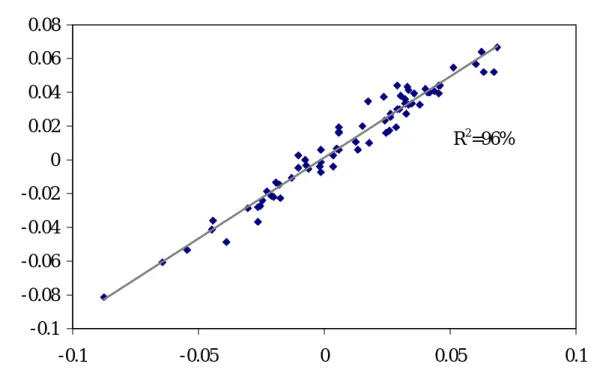
example, Figure 2 illustrates the time-series regression analysis for one fund from our

sample. In this case, the R2 is extremely high.

Specifically, the policy return can explain 96% of the variability of total fund return over time. In other words, the fund manager closely adhered to his or her policy target, deviating only marginally from the passive benchmark. SURZ, STEVENS, and WIMER (1999)

sub-tract the R2 value from one (1 − R2) to define

the level of conviction of the manager. A

man-ager with low (high) R2 has a low (strong)

conviction because he or she is willing (not willing) to make significant bets away from the benchmark. This leads to a return series that is well (not well) explained by the benchmark return. They use this terminology to clearly distinguish conviction from the importance of asset allocation for the magnitude of fund re-turns.

Table 1: Descriptive Statistic of Mutual Funds Asset Classes (all Returns in Euro)

German funds Swiss funds Mean return in % p.a. 10.88 9.70 Volatility in % p.a. 9.61 6.65 Benchmark returns: Mean in % p.a. Volatility in % p.a. Stocks:

MSCI Europe ex CH 19.32 15.42 MSCI Switzerland 18.39 17.25 MSCI North America 25.12 19.58 MSCI Asia Pacific 2.64 21.70 Bonds:

SB Europe ex CH and Ger 12.33 4.05 SB Germany 6.51 2.79 SB Switzerland 6.18 5.23 SB United States 16.32 9.60 SB Japan 6.26 12.56 Cash: Euro 5.26 1.11 German mark 3.72 0.13 Swiss franc 3.30 3.52 U.S. dollar 14.68 9.43 U.K. pound 13.18 7.84

(7)

Table 2 shows the average and median R2s

over all funds. The average R2 is 82.9%, the

median is 85.7%. Our results confirm the BRINSON et al. (1986, 1991) and IBBOTSON and KAPLAN (2000) results for U.S. data. In their first study, BRINSON, SINGER and BEEBOWER (1986) used a sample of 91 large U.S. pension funds over a period of 10 years

from 1974 to 1983. They report an average R2

of 93.6%. In their second study, BRINSON, SINGER and BEEBOWER (1991) used 82 large U.S. pension funds over another 10 years

from 1978 to 1987. They report an average R2

of 91.5% for this more recent sample period. IBBOTSON and KAPLAN (2000) worked with two different samples: (i) quarterly returns of 58 U.S. pension funds from 1993

to 1997, resulting in an average R2 of 88%,

Table 2: Comparisons of Time-Series Regressions

Brinson (1986) Brinson (1991) Ibbotson/Kaplan (2000) This study Type Pension funds Pension funds Pension funds Mutual funds Mutual funds R2

Average 93.6% 91.5% 88.0% 81.4% 82.9% Median NA NA 90.7% 87.6% 85.7% Active return (AR) p.a.

Average –1.1% –0.1% –0.44% –0.27% –2.37% Median NA NA 0.18% 0.00% –2.00% Figure 1: Time-Series Regression of Fund Returns versus Policy R eturns

R

2

=96%

-0.1 -0.08 -0.06 -0.04 -0.02 0 0.02 0.04 0.06 0.08 -0.1 -0.05 0 0.05 0.1

Policy return in % per month

Fund r et u rn i n % per m ont h Fu n d re tu rn i n % p er m o n th R2=96%

(8)

Table 3: Percentiles of Time-Series R2s

Ibbotson/Kaplan (2000) This study Data Pension funds Mutual funds Mutual funds Percentiles 5% 66.2% 46.9% 57.7% 25% 94.1% 79.8% 77.4% 50% 90.7% 87.6% 85.7% 75% 94.7% 91.4% 92.3% 95% 97.2% 94.1% 95.5%

and (ii) monthly returns for 94 U.S. balanced mutual funds from 1988 to 1998, resulting in

an average R2 of 81.4%. We conclude that the

degree of active management is similar in the U.S. and continental Europe.

However, Table 2 also shows a striking differ-ence in the magnitudes of active returns. Whereas the studies for the U.S. exhibit active returns of roughly zero (which is consistent with market efficiency), we report negative active returns of –2.37% per year for German and Swiss mutual funds. While the degree of active management is similar, the importance of asset allocation for the level of fund returns (or better, the quality of active management) is obviously very different. While U.S. fund man-agers could not add value by deviating from their benchmarks and/or picking tomorrow’s Microsofts, active asset management by Ger-man and Swiss fund Ger-managers actually de-stroyed value. One reason for this difference could be that we did not adjust for currency risk. Whereas foreign investments account for only 2.1% in the IBBOTSON and KAPLAN

study, the respective portion is 32.8% in our sample. The spread in the percentage of for-eign investments across funds in our sample is substantial. Intuitively, currency risk will have a bigger influence for those funds with a high proportion of foreign assets. To get a better idea of the differences in results across funds, Table 3 shows the percentiles of time-series R2s.

In a next step, we consider that the time-series

R2s may be simply high because funds

partici-pate in the capital markets and not because fund managers follow their specific asset allo-cation policies. To answer this question, we run two additional regressions for each fund: (i) a regression of total fund returns on the MSCI world benchmark, and (ii) a regression of total returns on average policy returns over all funds (instead of each fund’s return against the return on its own policy benchmark).

Table 4 displays the results. In contrast to

IBBOTSON and KAPLAN (2000), the R2s

are significantly below those reported in Table 2.

Table 4: Explanatory Power of Different Benchmarks

MSCI World Average policy over all funds Specific fund policy R2

Average 56.7% 63.9% 82.9%

(9)

With the MSCI world market index as the

benchmark for all funds, the average R2 is

56.7% and the median is 66.5%. Interestingly, even when using the average policy returns over all funds as the common benchmark, the

mean and median R2s (63.9% and 74.2%,

re-spectively) are still considerably lower com-pared to the values when the specific fund

policies are used. Hence, the high R2s in the

time-series regressions stem to a large extent from the funds’ participation in the capital markets. Nevertheless, the specific asset allo-cation policies are important determinants of funds’ time-series variability.

5.2 Variation among Funds

To compare the variation in returns attribut-able to asset allocation policy among funds, we apply a cross-sectional regression analysis. As

discussed above, when all funds followed the same passive asset allocation policy, there would be no variation among funds, but the asset allocation policy explains all of the time-series variability of a fund’s return. In contrast, if all funds were invested passively but had a wide range of asset allocation poli-cies, all of the variation in returns would be attributable to policy. Accordingly, the two

factors that drive the cross-sectional R2

are (i) the differences between the funds’ asset allocation policies (i.e., differences in their benchmarks) and (ii) the differences in the de-gree of active timing and/or stock picking. We have found as an answer to the first question that the degree of active management is similar for U.S. and German/Swiss fund managers. Therefore, a possible difference in our cross-sectional explanatory power should come from differences in the breadth of mutual fund products.

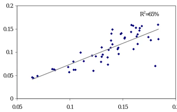
Figure 2: Cross-Sectional Regression of Fund Returns versus Policy R eturns

R

2

=65%

0 0.05 0.1 0.15 0.2 0.05 0.1 0.15 0.2

Compound average policy return in % p.a.

Co m pound aver age f und r et u rn i n % p. a Co m p o u nd a v er a g e f u nd r et u rn in % p .a . R2=65%

(10)

As explained in equations (6) and (7), we compute for each fund the geometric average annual total return and the geometric average annual policy return. These values are com-pared over all funds in a cross-sectional

re-gression. The resulting R2 is 65%, as

illus-trated in Figure 2. This implies that policy ex-plains, on average, 65% of the variation of re-turns across funds, and the remaining 35% is explained by timing and/or stock picking abili-ties. This number is considerably higher than the 40% cross-sectional explanatory power re-ported in IBBOTSON and KAPLAN (2000).

As discussed above, the cross-sectional R2

de-pends (i) on how much the asset allocation policies of funds differ and (ii) on how much funds engaged in active management. To as-sess how much asset allocation policies differ among funds, Table 5 shows the cross-sectional averages, standard deviations, and different percentiles of the benchmark weights of the mutual funds. The large standard deviations of

target weights and the large spreads between percentiles show that there are substantial differences in the asset allocation policies among funds. Consistent with our higher sectional explanatory power, the cross-sectional standard deviations of policy weights are somewhat lower than the numbers provided

by IBBOTSON and KAPLAN (2000).[11]

To assess how the degree of active

manage-ment affects the cross-sectional R2 in our

sam-ple, we replicate the approach in IBBOTSON and KAPLAN (2000) and compute the

cross-sectional R2 using a set of modified fund

re-turns. Intuitively, more active fund

manage-ment will result in a lower cross-sectional R2.

A modified return is defined as a weighted av-erage of the actual fund return and the return on the policy benchmark:

(

)

it it * it x TR 1 x PR R = ⋅ + − ⋅ , (8) where * it

R denotes the modified return on fund i.

Table 5: Cross-Sectional Distribution of Asset Class Weights (in %)

Mean Vola Percentile

5 25 50 75 95

Stocks:

MSCI Europe ex CH 22.86 17.93 1.01 11.63 19.51 31.81 54.75 MSCI Switzerland 4.43 7.22 0.00 0.00 0.39 5.64 19.51 MSCI North America 7.04 8.40 0.00 0.00 6.15 10.08 24.36 MSCI Asia Pacific 5.71 4.62 0.00 1.77 4.96 8.76 14.68 Bonds:

SB Europe ex CH and Ger 7.01 11.93 0.00 0.00 2.53 8.13 27.62 SB Germany 17.47 18.47 0.00 0.00 10.91 28.50 53.08 SB Switzerland 8.80 13.98 0.00 0.00 2.75 9.41 39.77 SB United States 16.49 22.16 0.00 2.16 5.96 19.71 70.28 SB Japan 0.44 0.98 0.00 0.00 0.00 0.04 2.98 Cash: Euro 1.50 3.27 0.00 0.00 0.00 0.12 10.00 German mark 1.36 3.13 0.00 0.00 0.00 0.00 9.88 Swiss franc 2.56 4.32 0.00 0.00 0.00 5.56 10.00 U.S. dollar 3.15 4.18 0.00 0.00 0.00 7.91 10.00 U.K. pound 1.19 2.71 0.00 0.00 0.00 0.14 7.66

(11)

The value of x sets the level of active manage-ment. Setting x to 1 delivers the sample result. A value of x below 1 reduces the level of ac-tive management below what the funds in the sample actually did. In contrast, a value of x above 1 implies that fund managers short the benchmark and take a levered position in the fund, thereby increasing the level of active management beyond the actual level. The com-pound annual return of modified fund returns was calculated as the geometric mean of the modified annual returns.

Figure 3 shows the influence of fund managers’

activity on the cross-sectional R2. We perform

regressions of the modified compound annual

returns on compound annual policy returns for various values of x. With x equal to 1, the modified return and the actual return are the

same. This has led to an R2 of 65% for our

sample. If the funds had been half as active

(x = 0.5), the R2 would have been much higher

with roughly 90%. In contrast, if the funds had been one-and-a-half times as active (x = 1.5),

the R2 would have been only 50%. This clearly

demonstrates that the degree of active man-agement strongly affects the cross-sectional

R2. However, the effect is not as pronounced

as in the IBBOTSON and KAPLAN (2000)

study. For example, they report an R2 of 14%

for x = 1.5.

Figure 3: Degree of Active Management versus Cross-Sectional R2

Mutual fund sample (65%)

Less active More active

0% 10% 20% 30% 40% 50% 60% 70% 80% 90% 100% 0.0 0.5 1.0 1.5 2.0

Degree of active management

Cr o ss -s ect iona l R 2

(12)

5.3 Return Level

The third question asks what portion of the return level is explained by asset allocation policy returns. Many people mistakenly re-ferred to the BRINSON et al. studies, arguing that the correct answer would be around 90%. However, SURZ, STEVENS, and WIMER (1999) strongly argue that the explanatory power of asset allocation for performance pertains to the magnitude of returns, not the variability of returns. Therefore, we compute the percentage of fund return explained by policy return for each fund as the ratio of

compound annual policy return, PR , divided_i

by the compound annual total return, R . This_i

ratio will be one if a fund followed exactly its policy mix and invested passively. A fund that outperformed (underperformed) will have a ratio less (larger) than 1. In fact, this ratio of compound returns is a performance measure: like the active return part in question 1 (but unlike question 2), this question asks whether active asset management can add value.

Table 6 reports the average and median ratios. As in IBBOTSON and KAPLAN (2000), pol-icy accounted for more than all of the total returns. However, in contrast to their results, active management not only failed to add value above the policy benchmarks. In fact, it de-stroyed a significant portion of investors’ value. A median ratio of 134% implies that ac-tive management destroyed roughly 25% of the performance that would have been achieved, on average, following a passive strategy.

Our results must be driven by a combination of timing, security selection, management fees, and expenses. Management fees and expenses are much higher in Germany and Switzerland, however, the difference seems too large to be explained by these two factors only. As in the answer to the first question, we conclude that the quality of active management in our sample of German and Swiss balanced mutual funds is inferior compared to the sample of U.S. funds examined in IBBOTSON and KAPLAN (2000). The distribution of the percentage of fund returns explained by policy returns (in levels) is shown in Table 7. The results are slightly better for the managers in the top 5% percentile, but even here the ratio is slightly above 1. The underperformance of the fund managers in the bottom 5% percentile is more than surprising: the performance ratio is as

high 180%![12]

SHARPE (1991) argues that because the aggre-gation of all investors is the market, the aver-age performance before costs of all investors must equal the performance of the market. Be-cause costs do not net out across investors, the average investor must underperform the mar-ket on a cost-adjusted basis. The implication is that, on average, more than 100% of the level of fund return would be expected from policy return. Of course, this outcome is not assured for subsamples of the market, such as balanced mutual funds. Indeed, our sample is clearly only a small subsample of the market (e.g., we do not include pension funds and individual investors), but the coverage within the mutual fund segment is sufficiently complete. Therefore,

Table 6: Percent of Total Return Level Explained by Policy Return

Brinson (1986) Brinson (1991) Ibbotson/Kaplan (2000) This study Type Pension funds Pension funds Pension funds Mutual funds Mutual funds Average 112% 101% 99% 104% 134% Median NA NA 99% 100% 131%

(13)

Table 7: Percentiles of Total Return Level Explained by Policy Return

Ibbotson/Kaplan (2000) This study Data Pension funds Mutual funds Mutual funds Percentiles 5% 82% 86% 101% 25% 94% 96% 114% 50% 100% 99% 131% 75% 112% 102% 144% 95% 132% 113% 180%

we believe that our results cannot simply be dismissed on the basis of a selection bias. Fi-nally, SURZ, STEVENS, and WIMER (1999) argue that just because the average impact of investment policy should be near 100%, active management is not necessarily worthless. In the end, half the managers are better than av-erage. But given the results in Table 7, it is more than questionable whether it pays off to expend efforts selecting the better-than-average fund managers in our sample of Ger-man and Swiss balanced mutual funds.

6. Conclusions

In this paper we analyse the contribution of as-set allocation policy to the performance of 51 German and Swiss balanced mutual funds. While it is well known that asset allocation policy is the major determinant of total fund performance, there is substantial disagreement about the exact magnitude. Following the ap-proach in IBBOTSON and KAPLAN (2000), we demonstrate that the correct answer de-pends on the specific question being asked. We find that more than 80 percent of the variabil-ity in returns of a typical fund over time is ex-plained by asset allocation policy, roughly 60 percent of the variation among funds is ex-plained by policy, and more than 130 percent of the return level is explained, on average, by the policy return level. Comparing our

empiri-cal results to previous results by BRINSON et al. (1986, 1991) and IBBOTSON and KAP-LAN (2000) for U.S. pension fund and mutual fund data, we come to three conclusions. First, we find that the degree of active management is similar. Second, we document evidence that U.S. managers offer a more diverse range of mutual fund products, i.e., compared to our sample of German and Swiss funds, there are more pronounced differences in the asset allo-cation targets among funds. Finally, we report that, on average, active management (i.e., stock picking and/or timing) has not even been neutral to fund performance, but rather de-stroyed a significant portion of investors’ value.

(14)

FOOTNOTES

[1] See HENSEL, EZRA and ILKIV (1991).

[2] See DROBETZ (2001) for an accessible intro-duction.

[3] See IBBOTSON and KAPLAN (2000), p.26. [4] See Sharpe (1992), p.8.

[5] From discussions with fund managers we in-ferred that they attempted to hold no more than 10% in cash. Therefore, we introduce the addi-tional restriction that the total cash holdings must not exceed 10% in our optimization. [6] LUCAS and RIEPE (1996) provide a good

de-scription of the empirical problems in the im-plementation of style analysis.

[7] To account for the approximate cost of repli-cating the policy mix through indexed funds we deduct 0.2% per year from the policy return. [8] Funds are classified as Swiss or German if they

are offered to residents in either country. For tax reasons, some funds are managed in Swit-zerland or Germany, but registered under Lux-embourg law.

[9] Empirically, asset classes can be determined applying mean-variance spanning tests. See FERSON, FOERSTER and KEIM (1993) and DESANTIS (1995) for recent examples.

[10] For example, see WYDLER (1998).

[11] See their Table 5 on p. 31. One reason could be that the cash positions in their portfolios are not restricted. However, we apply the 10% re-striction on the total weights on cash given in-formation from the fund guides and our inter-views with eight fund managers.

[12] To make sure these results are not driven by our restriction on the weights of cash, we repli-cated all computations without the 10% con-straint on money deposits. Intuitively, relaxing the constraints on cash should decrease the policy return and, hence, lead to lower ratios in Table 6. However, the results do not change significantly; the mean ratio is 130%, the me-dian ratio 129%.

BIBLIOGRAPHY

BLACK, F. and R. LITTERMAN (1992): “Global Portfolio Optimization”, Financial Analysts Journal (September–October), pp. 28–43.

BRINSON, G., L. HOOD and G. BEEBOWER (1986): “Determinants of Portfolio Performance”, Fi-nancial Analyst Journal (July/August), pp. 39–48. BRINSON, G., B. SINGER and G. BEEBOWER (1991): “Determinants of Portfolio Performance II: An Update”, Financial Analyst Journal (May/June), pp. 40–48.

DE SANTIS, G. (1995): “Volatility Bounds for Sto-chastic Discount Factors; Tests and Implications from International Financial Markets”, Working Pa-per, Marshall School of Business, University of Southern California.

DROBETZ, W. (2001): “Avoiding the Pitfalls in Portfolio Optimization: Putting the Black-Littermann Approach at Work”, Financial Markets and Portfolio Management, pp. 59–75.

FERSON, W. E. and C. R. HARVEY (1993): “The risk und predictability of international equity returns”, The Review of Financial Studies 6, pp. 527–566. FERSON, W, S. FOERSTER and D. KEIM (1993): “General test of latent variable models and mean-variance spanning”, Journal of Finance 48, pp. 131– 156.

FONDSFÜHRER SCHWEIZ (2001), Lipper.

FONDSGUIDE DEUTSCHLAND: Ratgeber Invest-mentfonds (2000), Gesellschaft für Fonds-Analyse (GFA), Schäffer-Poeschel.

HENSEL, C., D. EZRA und J. ILKIW (1991): “The importance of the Asset Allocation Decision”, Fina n-cial Analyst Journal (July/August), pp. 65–72.

Hoppenstedt Fondsführer (2000), Verlag Hoppen-stedt.

IBBOTSON, R. and P. KAPLAN (2000): “Does Asset Allocation Policy Explain 40, 90 or 100 Percent of Performance”, Financial Analyst Journal (Janu-ary/February), pp. 26–33.

LUCAS, L. and M. RIEPE (1996): “The role of returns-based style analysis: Understanding, implementing, and interpreting the techni-que”, Working Paper, Ibbotson Associates, http: //www.ibbotson.com/ rsearch/papers/mutual.asp

(15)

SHARPE, W. (1991): “The Arithmetic of Active Management”, Financial Analyst Journal (Janu-ary/February), pp. 7–9.

SHARPE, W. F. (1992): “Asset allocation: Manage-ment style and performance measureManage-ment”, Journal of Portfolio Management (Winter), pp. 7–19.

SURZ, R., D. STEVENS and WIMER M. (1999): The importance of Investment Policy, Journal of Invest-ing (Winter), pp. 80–85.

WYDLER, D. (1998): „Zur Auswirkung des Euro auf die Anlagestrategie“, Finanzmarkt und Portfolio-management, pp. 119–123.