Measuring Malware Evolution Using Support Vector Machines

(1)

San Jose State University

SJSU ScholarWorks

Master's Projects Master's Theses and Graduate Research

Spring 5-21-2019

Measuring Malware Evolution Using Support

Vector Machines

Mayuri Wadkar

San Jose State University

Follow this and additional works at:https://scholarworks.sjsu.edu/etd_projects

Part of theArtificial Intelligence and Robotics Commons, and theInformation Security Commons

This Master's Project is brought to you for free and open access by the Master's Theses and Graduate Research at SJSU ScholarWorks. It has been accepted for inclusion in Master's Projects by an authorized administrator of SJSU ScholarWorks. For more information, please contact [email protected].

Recommended Citation

Wadkar, Mayuri, "Measuring Malware Evolution Using Support Vector Machines" (2019).Master's Projects. 708. DOI: https://doi.org/10.31979/etd.ed7k-dh6a

(2)

Measuring Malware Evolution Using Support Vector Machines

A Project Presented to

The Faculty of the Department of Computer Science San José State University

In Partial Fulfillment

of the Requirements for the Degree Master of Science

by

Mayuri Wadkar May 2019

(3)

(4)

The Designated Project Committee Approves the Project Titled

Measuring Malware Evolution Using Support Vector Machines

by

Mayuri Wadkar

APPROVED FOR THE DEPARTMENT OF COMPUTER SCIENCE

SAN JOSÉ STATE UNIVERSITY

May 2019

Dr. Mark Stamp Department of Computer Science

Prof. Fabio Di Troia Department of Computer Science

(5)

ABSTRACT

Measuring Malware Evolution Using Support Vector Machines by Mayuri Wadkar

Malware is software that is designed to do harm to computer systems. Malware often evolves over a period of time as malware developers add new features and fix bugs. Thus, malware samples from the same family from different time periods can exhibit significantly different behavior. Differences between malware samples within a single family can originate from various code modifications designed to evade signature-based detection or changes that are made to alter the functionality of the malware itself. In this research, we apply feature ranking based on linear support vector machine (SVM) weights to identify, quantify, and track changes within malware families over time. We analyze numerous malware families over an extended period of time. Our goal is to detect and analyze evolutionary changes over a wide variety of malware families using quantifiable and automated machine learning techniques.

(6)

ACKNOWLEDGMENTS

It is my sincere pleasure to acknowledge the guidance of my graduate advisor Dr. Mark Stamp who provided knowledge, encouragement, feedback and valuable time. His insights and constructive criticism improved this report enormously.

I would also like to thank my committee members Prof. Fabio Di Troia and Dr. Thomas Austin for their valuable feedback and time.

Last but foremost, I would like to thank my dear husband for being patient and supporting me.

(7)

TABLE OF CONTENTS

CHAPTER

1 Introduction . . . 1

2 Related Work . . . 3

3 Design and Implementation . . . 5

3.1 Dataset . . . 5

3.1.1 Malware Families . . . 6

3.1.2 Portable Executable File Format . . . 8

3.2 Feature Extraction . . . 9

3.2.1 Byte 𝑁-Grams . . . 9

3.2.2 Features Extracted From PE Files . . . 9

3.3 Support Vector Machine . . . 10

3.3.1 Feature ranking based on weights from linear SVM . . . . 11

3.4 Decision Tree . . . 11

3.5 Chi-Squared Statistic . . . 12

3.6 Experimental Approach . . . 13

4 Experiments and Results . . . 14

4.1 System Configuration . . . 14

4.2 Zbot Malware Family . . . 14

4.2.1 SVM based experiment using byte 𝑛-gram features . . . . 14

4.2.2 SVM experiment using PE file based features . . . 17

(8)

4.3 Chi-Squared Statistic . . . 21

4.4 Experiment With Two Similar Malware Families . . . 23

4.5 Experiment With Two Dissimilar Malware Families . . . 24

5 Conclusion and Future Work . . . 26

5.1 Conclusion . . . 26

5.2 Future Work . . . 26

LIST OF REFERENCES . . . 27

APPENDIX Additional Results . . . 32

A.1 Vobfus Malware Family . . . 32

A.1.1 SVM based experiment using byte 𝑛-gram features . . . . 32

A.1.2 SVM experiment using PE file based features . . . 33

A.2 Hotbar Family . . . 35

A.3 Vbinject Family . . . 36

A.4 Winwebsec Family . . . 37

A.5 DelfInject Family . . . 39

A.6 Rbot Family . . . 40

A.7 Obfuscator Family . . . 42

A.8 Bifrose Family . . . 43

A.9 Zegost Family . . . 45

A.10 Dorkbot Family . . . 46

A.11 Hupigon Family . . . 48

(9)

LIST OF TABLES

1 Number of samples used in the experiments. . . 5

2 Features extracted from PE files . . . 10

3 Indices of top 5 features with the largest variation in weight. . . . 16

4 Top 3 PE based features with largest variation in weight. . . 19

5 Number of samples used in the experiment. . . 23

(10)

LIST OF FIGURES

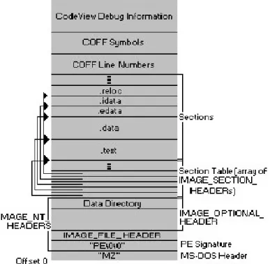
1 The PE File Format. . . 8

2 Byte 𝑁-Gram Feature Extraction. . . 9

3 Zbot: Raw weights of𝑛-gram features from linear SVM. . . 15

4 Zbot: Average weights of individual 𝑛-gram features from linear SVM. . . 15

5 Zbot: Chi-square Statistic. . . 17

6 Zbot: Raw feature weights from linear SVM. . . 18

7 Zbot: Average weights of individual features from linear SVM. . . 18

8 Zbot: Chi-square Statistic. . . 19

9 Zbot: Feature importances from Decision Tree Classifier. . . 20

10 Zbot: Feature importances from Decision Tree Classifier. . . 21

11 Vbinject: Chi-squared statistics. . . 22

12 Hotbar: Chi-squared statistics. . . 22

13 CeeInject-Vbinject: Chi-squared statistics. . . 23

14 Zbot-Hotbar: Chi-squared statistics. . . 24

A.15 Vobfus: Raw weights of 𝑛-gram features from linear SVM. . . 32

A.16 Vobfus: Average weights of individual 𝑛-gram features from linear SVM. . . 33

A.17 Vobfus: Chi-square Statistic. . . 33

A.18 Vobfus: Raw feature weights from linear SVM. . . 34

A.19 Vobfus: Average weights of individual features from linear SVM. 34 A.20 Vobfus: Chi-square Statistic. . . 35

(11)

A.21 Hotbar: Raw feature weights from linear SVM. . . 35

A.22 Hotbar: Average weights of individual features from linear SVM. 36

A.23 Vbinject: Raw feature weights from linear SVM. . . 36

A.24 Vbinject: Average weights of individual features from linear SVM. 37

A.25 Winwebsec: Raw feature weights from linear SVM. . . 37

A.26 Winwebsec: Average weights of individual features from linear SVM. 38

A.27 Winwebsec: Chi-squared statistics. . . 38

A.28 DelfInject: Raw feature weights from linear SVM. . . 39

A.29 DelfInject: Average weights of individual features from linear SVM. 39

A.30 DelfInject: Chi-squared statistics. . . 40

A.31 Rbot: Raw feature weights from linear SVM. . . 40

A.32 Rbot: Average weights of individual features from linear SVM. . 41

A.33 Rbot: Chi-squared statistics. . . 41

A.34 Obfuscator: Raw feature weights from linear SVM. . . 42

A.35 Obfuscator: Average weights of individual features from linear SVM. 42

A.36 Obfuscator: Chi-squared statistics. . . 43

A.37 Bifrose: Raw feature weights from linear SVM. . . 43

A.38 Bifrose: Average weights of individual features from linear SVM. 44

A.39 Bifrose: Chi-squared statistics. . . 44

A.40 Zegost: Raw feature weights from linear SVM. . . 45

A.41 Zegost: Average weights of individual features from linear SVM. . 45

A.42 Zegost: Chi-squared statistics. . . 46

(12)

A.44 Dorkbot: Average weights of individual features from linear SVM. 47 A.45 Dorkbot: Chi-squared statistics. . . 47

A.46 Hupigon: Raw feature weights from linear SVM. . . 48

A.47 Hupigon: Average weights of individual features from linear SVM. 48

A.48 Hupigon: Chi-squared statistics. . . 49

A.49 CeeInject: Raw feature weights from linear SVM. . . 49

A.50 CeeInject: Average weights of individual features from linear SVM. 50

(13)

CHAPTER 1 Introduction

Malware is usually defined as "malicious software" aimed to cause disruption or denial of activity, gathering private data without consent, allowing unapproved access to system resources, and other improper behavior [1]. Malware detection and prevention is a top priority for governments and businesses. With recent advances in technology (GPUs, Cloud, BYOD/IOT devices, etc.) malware evasion is of great concern too.

Building countermeasures for these threats is becoming very difficult due to increasing complexity of network systems and software. Creators of malware are aware of the details about networks and security mechanisms incorporated in end hosts. They are developing even more sophisticated and effective methods for subverting them. Hackers, enthusiasts, and organized criminals frequently introduce new features intended to enable their malware to evade detection. It is very likely that newer malware is written based of existing ones rather than starting from scratch [2]. Hence, malware can be seen as evolving over time. Usually in software development process, new software is written on top of the existing software. Thus, malware writers be inclined to reuse existing malware code and release new variants of the same malware [3].

Staying informed and up to date on which threats are out there and how they work, will help in developing countermeasures. Thus, understanding malware evolution and identifying the relationship between various malware samples, is of great significance. It will help us to understand the connections among existing malware families and might also be useful to detect unknown malware. Earlier works used reverse engineering techniques to extract knowledge about unknown malware. Using reverse engineering, malware is broken down to reveal its inner workings, architecture, code segments, and

(14)

design. In this research, we will use a class of machine learning techniques to measure malware evolution for a wide variety of malware families.

Support vector machines (SVMs) are a popular technique for supervised learn-ing [4]. Feature ranklearn-ings based on the weights of a linear SVM can be used to eliminate features that contribute little to the model or to gain insight into the train-ing data [5]. In this research we conduct experiments ustrain-ing linear SVM and feature ranking technique to track and quantify changes within malware families over time. Decision tree (DT) algorithm starts at the tree root and splits the data on the feature that maximizes the information gain. Using this information gain we can determine which features from the given set are most important [4]. In this research, we use feature importances from trained decision tree classifier to validate and support SVM based analysis.

We have considered static features such as byte 𝑛-grams for training linear SVM. In addition to byte 𝑛-grams, we have used features extracted from binary representation of portable executable (PE) files to train linear SVM and DT classifiers.

This report is organized as follows. In Chapter 2, we discuss related work. Chapter 3 describes machine learning techniques used — SVM and decision trees. These techniques have been discussed briefly along with dataset, features, design, and implementation. Chapter 4 describes experimental results and analysis. In Chapter 5, we conclude our work and also discuss possible future work related to our research.

(15)

CHAPTER 2 Related Work

There are many experimental studies of malcode detection published until now. S. Attaluri et al. [6] consider using profile hidden markov models for detecting metamorphic malware. D. Lin and M. Stamp [7] explore shortcomings of hidden markov model (HMM) based detection approach. Similar techniques have been successfully applied for masquerade detection [8]. Singular value decomposition has been exercised in order to detect metamorphic malware [9]. The emphasis of these studies was on a specific area such as detection of metamorphic malware or masquerade detection. Numerous experimental studies of malware classification have been presented until now. However, very few attempts have been made to understand the evolution of malware variants of a specific family.

Evolutionary characteristics of malware have been investigated in [10, 11]. A research that construes the phylogeny of malware was published by Ma et al. [12]. Their techniques discovered significant amount of code sharing between different malware families and accurately captured subtle changes among variants of the same family. Their approach and results are useful in understanding the evolution of remote code injection malware. According to A. Gupta et al. [13], an instance of malware may give rise to many others. Few malware families are active for many years, while others are active for just a few days. Their research revealed many families where specific traits are inherited after many months. They used graph pruning technique to demonstrate inheritance relationships between different variants of malware.

Our research is similar to these studies as in we also aim to establish evolutionary relationships among malware variants. However, in contrast with previous studies, our work focuses on malware variants spanning many years allowing us to offer a broad view into the evolution of malware features. We use automated machine

(16)

learning techniques in contrast to the reverse engineering technique used by previous researchers.

Many researchers study broad sets of features like third-party calls [14], API-calls, string-based features [15], permissions and network addresses to distinguish the nature of applications. Such features are extracted from the sets of benign as well as malware samples to build detection tools. The study presented in [16] uses a different method for feature selection, in which 𝑛-grams are ranked based on frequency and entropy. Their work shows that a class-wise feature selection can improve model efficiency. It involves extracting the top k byte 𝑛-grams from samples and using those as the feature space. The research in [17] used a feature fusion technique to perform malware family classification. They used structural features such as 𝑛-grams, entropy, and image representation. Along with hex-dump based features, they also used features extracted from disassembled files such as opcodes, API calls, and sectional information of PE file. Their proposed method achieved a very high accuracy of approximately 0.998.

Byte 𝑛-grams are a popular feature type used in static analysis and have been used in many prior studies [18, 19, 20]. Dynamic analysis is not required in case of byte 𝑛-gram features. Without the knowledge of file format, these features enable analysts to learn great deal of information from header and other code sections of an executable file [21]. We also leverage the effectiveness of𝑛-gram features in our project. This literature review helped us in choosing the appropriate features and machine learning techniques for our experiments.

(17)

CHAPTER 3

Design and Implementation

In this chapter, we first discuss about dataset and features used to conduct experiments. In later sections, we discuss about linear SVM, decision trees and the approach taken to analyze evolutionary changes in malware families.

3.1 Dataset

For this research, we used malware dataset comprised of 26,245 portable ex-ecutable (PE) files belonging to 13 different malware families. We used malware samples from families listed in Table 1. Each family represents a class of malware which share some traits in how they carry out an attack, their purpose, kind of information they target, how good they are at hiding themselves, etc. We introduce these malware families in Section 3.1.1.

Table 1: Number of samples used in the experiments.

Malware Family Number of samples Time Period (Year)

Zbot 1624 2010 – 2012 Vbinject 3715 2009 – 2012 Winwebsec 1460 2011 – 2012 DelfInject 281 2010 – 2012 Rbot 782 2004 – 2007 Hotbar 2437 2011 – 2012 Obfuscator 2707 2004 – 2011 Bifrose 1048 2010 – 2012 Zegost 2452 2010 – 2012 Dorkbot 526 2010 – 2012 Hupigon 1442 2007 – 2011 Vobfus 6643 2010 – 2012 CeeInject 1128 2009 – 2012

In order to conduct experiments in an efficient manner, the dataset was organized in such a way that malware samples belonging to the same family were kept in the same directory. These were further split into sub-directories based on compilation

(18)

month and year of the PE files. Malware samples with altered compilation date or creation date were discarded during initial wrangling process of the dataset.

3.1.1 Malware Families

Zbot is a trojan horse that tries to steal confidential information from a compromised computer. It explicitly targets system data, online sensitive data, and banking information, yet can be modified through the toolbox to accumulate any kind of data. The trojan itself is basically disseminated through drive-by downloads and spam campaigns. It was first discovered in January 2010 [22].

VBinject comprises of worms and trojans that disguise other malware inside it.

VBinject is a packaged malware, i.e. a malware that utilizes encryption and compression programming to obscure its contents. Hence, it is hard to recognize other malware that it is concealing. It was first seen in 2009 and again in 2010 [23].

Winwebsec trojan presents itself as an antivirus software. It shows misleading

messages to the users stating that the device has been infected and persuades them to pay for the bogus product [24].

DelfInject worm enters a system as a file passed by other malware or as a file

downloaded accidentally by clients when visiting malignant sites. DelfInject drops itself on to the system using an arbitrary document name, (for example,

xpdsae.exe). It changes the registry entry, hence it runs at each system start. It then injects code intosvchost.exeso it can create a connection with specific servers and download files [25].

Rbot is a backdoor trojan that enables attacker to control the computer using an IRC channel. It then spreads to other computers by scanning for network

(19)

shares exploiting vulnerabilities in the system. It allows attackers to launch denial-of-service (DoS) attacks [26].

Hotbar is an adware program that installs itself on user’s computer or may be

downloaded by user from malicious website. It displays advertisements as user browses the web [27].

Obfuscator hides its purpose through obfuscation. The underlying malware can

have any purpose [28].

Bifrose is a backdoor trojan that allows attacker to connect to a remote IP using

random port number. Some variants of Bifrose have capability to hide files and processes from user. Attacker can view system information, retrieve passwords, or execute files by gaining remote control of the system [29].

Zegost is a backdoor trojan that injects itself into svchost.exeallowing attacker to

execute files on the compromised system [30].

Dorkbot is a worm that steals user names and passwords by keeping tab on what

user does online. It blocks security update websites and can launch DoS attack. It spreads through instant messaging applications, social networks, and flash drives [31].

Hupigon is a main component of family of backdoor trojans. It opens a backdoor

server enabling other remote computers to control a compromised system [32].

Vobfus malware family downloads other malware onto user’s computer. It uses

Windows Autorun feature to spread to other devices like flash drive. It makes long lasting changes to device configuration that cannot be easily restored just by removing the threat [33].

(20)

CeeInject aims to conceal its motivation in order to prevent detection by security programming software. Many malware families use it as a shield to prevent detection. It can obfuscate a bitcoin mining client, which might be installed on a system to mine bitcoins without the user’s knowledge [34].

3.1.2 Portable Executable File Format

Figure 1: The PE File Format.

This file format is supported by Windows and is an extension of the Common Object File format. We can obtain useful information from executable files such as their compilation time, size of data, number of imports, characteristics, version information, etc. The structure of a typical PE file is shown in Figure 1. The PE design specification allowed us to create a parser to extract features from the executable file and forms the basis for our static analysis. Each component of a PE file has specific standard which can be found at [35]. Files that divert from the given standards might be malicious or infected.

(21)

3.2 Feature Extraction

For our initial SVM based static analysis, experiments conducted use byte𝑛-gram features extracted from binary form of executable files. Later, the same experiments are repeated using a set of 55 features extracted from portable executable files.

3.2.1 Byte 𝑁-Grams

Byte n-grams are extracted by considering a file as a sequence of bytes. From this sequence, every possible unique combination of n successive bytes is considered as a separate feature. First we read each malware file as sequence of bytes and extracted byte 𝑛-grams. Top 𝑘 byte 𝑛-grams that occurred most frequently in the samples formed our feature space. The 𝑛-gram frequencies for each malware file form our feature vectors. For every malware file, feature vector was normalized by dividing each cell by the total number of bytes read from that file. The process is summarized in Figure 2. For all our experiments, we considered byte bi-grams (𝑛=2) as features.

Figure 2: Byte 𝑁-Gram Feature Extraction.

3.2.2 Features Extracted From PE Files

We extracted 55 novel features from PE files of malware samples which are listed in Table 2. This set of features was used to further enhance our SVM based analysis and results.

(22)

Table 2: Features extracted from PE files

Sr. No. Features Sr. No. Features

1. Machine 29. Size of Optional Header

2. Characteristics 30. Time Date Stamp

3. Major Linker Version 31. Minor Linker Version

4. Size of Code 32. Size of Initialized Data

5. Size of Uninitialized Data 33. Address of Entry Point

6. Base of Code 34. Base of Data

7. Image Base 35. Section Alignment

8. File Alignment 36. Major Operating System Version

9. Minor Operating System Version 37. Major Image Version

10. Minor Image Version 38. Major Subsystem Version

11. Minor Subsystem Version 39. Size of Image

12. Size of Headers 40. Checksum

13. Subsystem 41. Dll Characteristics

14. Size of Stack Reserve 42. Size of Stack Commit

15. Size of Heap Reserve 43. Size of Heap Commit

16. Loader Flags 44. Number of Rva and Sizes

17. Number of Sections 45. Mean Entropy of Sections

18. Minimum Entropy of Sections 46. Maximum Entropy of Sections

19. Mean Raw Size of Sections 47. Minimum Raw Size of Sections

20. Maximum Raw Size of Sections 48. Mean Virtual Size of Sections

21. Minimum Virtual Size of Sections 49. Maximum Virtual Size of Sections

22. Number of DLL Imports 50. Total Number of Imports

23. Ordinal Number of Imports 51. Number of Exports

24. Number of Resources 52. Mean Entropy of Resources

25. Minimum Entropy of Resources 53. Maximum Entropy of Resources

26. Mean Size of Resources 54. Minimum Size of Resources

27. Maximum Size of Resources 55. Load Configuration Size

28. Version Information Size

3.3 Support Vector Machine

Support vector machine (SVM) is one of the popular techniques for supervised learning and is used for data classification. It establishes a separating hyperplane by widening the separation between two classes of data [4]. Using SVM we can delineate input data to a higher dimensional feature space. SVM solves the following minimization problem given a set of instance-label pairs (𝑥𝑖, 𝑦𝑖), 𝑥𝑖 ∈𝑅𝑛,𝑦𝑖 ∈ {1,−1}, 𝑖= 1, . . . , 𝑙: min 𝑤,𝑏 1 2𝑤 𝑇_𝑤₊_𝐶 𝑙 ∑︁ 𝑖=1 𝜉(𝑤, 𝑏;𝑥𝑖, 𝑦𝑖), (1)

(23)

where 𝐶 ≥0 is a penalty parameter and 𝜉(𝑤, 𝑏;𝑥𝑖, 𝑦𝑖) is a loss function. The kernel function for linear SVM is given as 𝐾(𝑥𝑖, 𝑥𝑗) = 𝑥𝑇𝑖 𝑥𝑗. Our SVM experiments are based on a linear kernel function.

SVM trained model assigns weights to each feature used during the training phase. These weights can be used to decide the relevance of each feature [36]. Next subsection describes the feature ranking algorithm based on weights from linear SVM.

3.3.1 Feature ranking based on weights from linear SVM

Feature rankings based on the weights of a linear SVM can be used to eliminate features that contribute little to the model or to gain insight into the training data. These can be obtained by sorting the features according to the absolute values of weights in the model. Algorithm 1 briefly describes the steps involved in feature ranking technique.

Algorithm 1 Feature Ranking

Data: Training Set 𝑥𝑖, 𝑦𝑖 where 𝑖= 0,1, . . . , 𝑛.

Result: List of feature ranks in sorted order.

1: Train linear SVM on the given training set.

2: Rank features from 1 to 𝑛 based on absolute weights |𝑤𝑗| where 𝑗 = 0,1, . . . , 𝑛 assigned by SVM.

3: Sort feature ranks in ascending order. 4: Return top 𝑘 ranked features.

The value of |𝑤𝑗| is directly proportional to the significance of𝑗th feature. Thus, features are ranked using |𝑤𝑗|values [36]. However, this approach is limited to linear SVM.

3.4 Decision Tree

In decision trees, classification of samples start at root node and samples are sorted based on their feature values. Decision tree splits the dataset samples into smaller subsets in order to predict the target value [37]. Each node in a tree mimics a

(24)

feature and each edge represents a decision. The algorithm learns how to best split the dataset using a greedy strategy by making series of locally optimum choices about which feature to use for the split. There are numerous measures for evaluating the goodness of a feature such as entropy [38] and gini index [39]. These are derived based on degree of impurity of the child nodes in a given tree [40]. Typically used impurity measures in practice are mentioned below.

Entropy is calculated as,

Entropy(𝑡) =−

𝑐−1

∑︁

𝑖=0

𝑝(𝑖|𝑡)𝑙𝑜𝑔2 𝑝(𝑖|𝑡) (2)

Gini index is calculated as,

Gini(𝑡) = 1−

𝑐−1

∑︁

𝑖=0

[𝑝(𝑖|𝑡)]2 (3)

Error is computed as,

Classification error(𝑡) = 1−max

𝑖 [𝑝(𝑖|𝑡)] (4)

The splitting of dataset continues until a predefined stopping criterion is met or no further gain can be achieved. These measures enable us to identify the importance of features.

3.5 Chi-Squared Statistic

Chi-squared statistic is used to compare the observed frequency distribution with the expected frequency distribution [41]. This technique was proposed by Pearson in 1900 [42]. In mathematical terms, it is a normalized sum of square deviation between observed and expected frequency distributions. It is calculated as,

𝜒2 = 𝑛 ∑︁ 𝑖=1 (𝑂𝑖−𝐸𝑖)2 𝐸𝑖 (5) where𝑛denotes the number of features or observations,𝜒2is the cumulative chi-square statistic, 𝑂𝑖 is observed value of 𝑖th instance, and 𝐸𝑖 is expected value of 𝑖th instance.

(25)

In our experiments, this statistic was used to calculate the power-divergence between SVM feature weights from a specific time period and the average feature weights.

3.6 Experimental Approach

This section describes an approach taken in order to analyze evolutionary changes that occurred in the malware family over period of time. We selected a malware family from the dataset and tagged each sample in this family according to the date

on which it was compiled. Then we trained a linear SVM based on byte 𝑛-gram

features over all samples from a one year time interval. Using this model, we then ranked all features based on the SVM weights. Next, we shifted ahead one month and again trained an SVM on all samples within a one year window, and again ranked the features. Continuing, we obtained a series of snapshots of ranked features based on overlapping sliding windows, each of one year duration and each offset by one month. We used this as a means to trace changes in the significance of various features and to quantify changes. This approach is useful in detecting slow evolutionary changes as well as sudden breaks in the evolution.

Next step was to be able to identify and investigate features of a malware family that undergo significant variation in terms of SVM weights when we shift the training window. Thus, we repeated experimental approach mentioned in previous paragraph using feature set described in Table 2. Choosing this feature set enabled us to analyze individual features and their importances.

(26)

CHAPTER 4 Experiments and Results

In this chapter, we present analysis and results for the experiments conducted as part of our research. Prior to that, we describe the configuration of system used to carry out those experiments.

4.1 System Configuration

Since our project involved working with malware, all experiments were conducted in a controlled virtual environment. The configuration for virtual machine is given below.

• Processor: Intel(R) Xeon(R) CPU E5-2620 v3 @ 2.40GHz • CPU: 8 vCPUs

• RAM: 24 GB

• Operating System: Ubuntu 18.04.1 LTS Linux (64 bit).

• Plots and charts were generated using matplotlib library in Python. • Python sklearn libraries were used for machine learning algorithms. • PE file based features were extracted using pefile library in Python. • N-Gram features extracted using N-Gram library in Apache Spark.

4.2 Zbot Malware Family

In this section, we discuss experiments conducted on 1624 malware samples from Zbot family. First we discuss results of SVM based experiments that use byte 𝑛-gram features. Next, we present results of SVM based experiments that use 55 features extracted from PE files. Lastly, we discuss results of decision tree related experiments.

4.2.1 SVM based experiment using byte 𝑛-gram features

Initially we trained linear SVM using byte𝑛-gram (𝑛=2) features of Zbot samples from one year time interval (Jan. 2011 – Jan. 2012). We recorded feature weights from this trained model. Next, we shifted ahead one month and again trained an

(27)

SVM on samples within one year time window (Feb. 2011 – Feb. 2012). In this way, we captured series on 12 snapshots, starting at Jan. 2011 and ending at Dec. 2012, based on overlapping sliding windows, each of one year duration and each offset by one month. Figure 3 shows a plot of raw feature weights from all overlapping time windows of size one year. Next, we computed average weights of each individual features across all time windows. The result can be seen in Figure 4.

Figure 3: Zbot: Raw weights of 𝑛-gram features from linear SVM.

(28)

On comparing Figure 3 and Figure 4, it appears that in certain time windows for certain features the variation in weight is significant. Thus, in order to gain insight of features that have considerably large variation in weight from the average value, we fetched indices of top 5 features that vary the most in given time window. Refer to Table 3 for corresponding result of Zbot family. From this result, we see that weights for 593rd _{and 974}th _{features vary the most in all time windows.}

Table 3: Indices of top 5 features with the largest variation in weight.

Time Window 1st ₂nd ₃rd ₄th ₅th Jan. 2011 – Jan. 2012 593 974 183 3507 2080 Feb. 2011 – Feb. 2012 593 974 3507 183 724 Mar. 2011 – Mar. 2012 593 974 183 3507 724 Apr. 2011 – Apr. 2012 593 974 183 3507 724 May 2011 – May 2012 593 974 3507 183 2080 Jun. 2011 – Jun. 2012 593 183 3507 2080 724 Jul. 2011 – Jul. 2012 593 974 183 3507 724 Aug. 2011 – Aug. 2012 593 974 183 3507 724 Sep. 2011 – Sep. 2012 593 974 3507 724 2080 Oct. 2011 – Oct. 2012 593 974 2080 724 2493 Nov. 2011 – Nov. 2012 593 974 3507 183 724 Dec. 2011 – Dec. 2012 593 974 183 3507 724

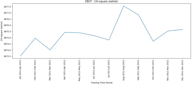
Further, we computed chi-squared statistics for feature weights obtained from all time windows, which can be viewed in Figure 5. Using this statistic, we can measure power-divergence of observed feature weights from average (i.e expected) feature weights. It indicates time windows in which significant changes were incorporated in malware samples. Based on our analysis in Figure 5, it appears that new Zbot variants were released in February 2012, April 2012, May 2012, August 2012, and November 2012. Such an analysis might help to understand release cycle of a specific malware family. Magnitude can denote the amount of evolution that has occurred during specific time period.

(29)

Figure 5: Zbot: Chi-square Statistic.

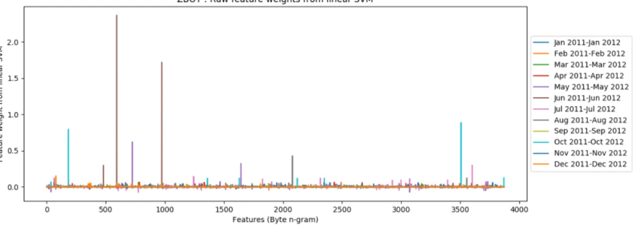
4.2.2 SVM experiment using PE file based features

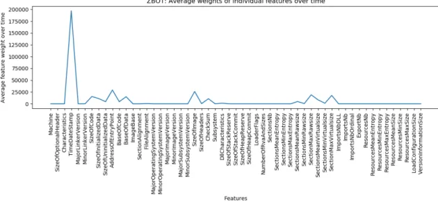
This experiment is based on Zbot samples compiled from year 2010 to year 2012. Initially, we trained SVM using 55 distinct features extracted from PE files of Zbot samples. Details about these features are given in Section 3.2.2. We captured linear SVM weights for multiple overlapping time windows. Along with raw feature weights, we also computed average weights of individual features. Corresponding results can be viewed in Figure 6 and Figure 7.

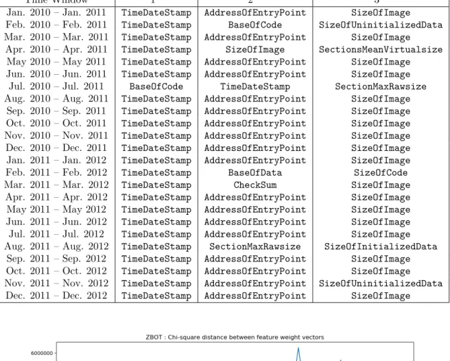
We observed that there exists a set of features for which the weight change is high in certain time windows. Next, we captured top 3 such features from each time window for which the variation is high. The result can be seen in Table 4. From this result, we see thatTimeDateStampfeature is the most prevalent across all selected time windows. As a similar feature was used to tag samples during SVM training, it is proof of concept that the SVM model used this feature to maximize the margin between classes. Features such as AddressOfEntryPoint and SizeOfImage also played vital role in the separation of classes. However, we can gain useful information from features other

(30)

Figure 6: Zbot: Raw feature weights from linear SVM.

Figure 7: Zbot: Average weights of individual features from linear SVM.

than prevalent features mentioned earlier. Because, these offer insight into attributes that might have been of interest to malware writers in certain time periods.

(31)

Table 4: Top 3 PE based features with largest variation in weight.

Time Window 1st ₂nd ₃rd

Jan. 2010 – Jan. 2011 TimeDateStamp AddressOfEntryPoint SizeOfImage

Feb. 2010 – Feb. 2011 TimeDateStamp BaseOfCode SizeOfUninitializedData

Mar. 2010 – Mar. 2011 TimeDateStamp AddressOfEntryPoint SizeOfImage

Apr. 2010 – Apr. 2011 TimeDateStamp SizeOfImage SectionsMeanVirtualsize

May 2010 – May 2011 TimeDateStamp AddressOfEntryPoint SizeOfImage

Jun. 2010 – Jun. 2011 TimeDateStamp AddressOfEntryPoint SizeOfImage

Jul. 2010 – Jul. 2011 BaseOfCode TimeDateStamp SectionMaxRawsize

Aug. 2010 – Aug. 2011 TimeDateStamp AddressOfEntryPoint SizeOfImage

Sep. 2010 – Sep. 2011 TimeDateStamp AddressOfEntryPoint SizeOfImage

Oct. 2010 – Oct. 2011 TimeDateStamp AddressOfEntryPoint SizeOfImage

Nov. 2010 – Nov. 2011 TimeDateStamp AddressOfEntryPoint SizeOfImage

Dec. 2010 – Dec. 2011 TimeDateStamp AddressOfEntryPoint SizeOfImage

Jan. 2011 – Jan. 2012 TimeDateStamp AddressOfEntryPoint SizeOfImage

Feb. 2011 – Feb. 2012 TimeDateStamp BaseOfData SizeOfCode

Mar. 2011 – Mar. 2012 TimeDateStamp CheckSum SizeOfImage

Apr. 2011 – Apr. 2012 TimeDateStamp AddressOfEntryPoint SizeOfImage

May 2011 – May 2012 TimeDateStamp AddressOfEntryPoint SizeOfImage

Jun. 2011 – Jun. 2012 TimeDateStamp AddressOfEntryPoint SizeOfImage

Jul. 2011 – Jul. 2012 TimeDateStamp AddressOfEntryPoint SizeOfImage

Aug. 2011 – Aug. 2012 TimeDateStamp SectionMaxRawsize SizeOfInitializedData

Sep. 2011 – Sep. 2012 TimeDateStamp AddressOfEntryPoint SizeOfImage

Oct. 2011 – Oct. 2012 TimeDateStamp AddressOfEntryPoint SizeOfImage

Nov. 2011 – Nov. 2012 TimeDateStamp AddressOfEntryPoint SizeOfUninitializedData

Dec. 2011 – Dec. 2012 TimeDateStamp AddressOfEntryPoint SizeOfImage

(32)

files. From Figure 8, it can be observed that feature weights in certain time windows diverted significantly from their average values. These time periods are April 2011, February 2012, May 2012, August 2012, and November 2012. Chi-squared statistics in Figure 5 and Figure 8 are identical. This indicates that our technique of detecting evolutionary patterns yields consistent results for both sets of features that are used in the analysis.

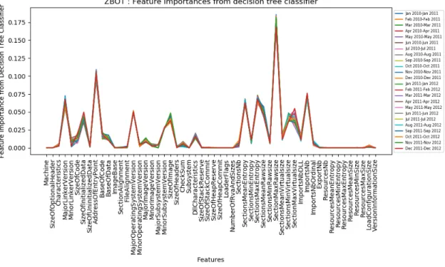
4.2.3 Decision tree based experiment using PE file features

Using the same 55 features as used in the SVM based analysis, we also trained decision tree classifier in order to obtain feature importances using entropy criterion. The purpose was to be able to relate these feature importances with corresponding feature weights obtained from linear SVM.

Figure 9 shows feature importances from decision tree classifier computed

us-ing entropy criterion for Zbot family. The model was trained on entire Zbot

dataset from all time windows at once. From this figure, we can notice certain features that are paramount for Zbot malware family such as SectionMaxRawSize,

AddressOfEntryPoint, etc.

(33)

Similar to SVM based analysis, we iteratively trained decision tree classifier on overlapping time windows. In Figure 10, we visualize feature importances from all time windows.

Figure 10: Zbot: Feature importances from Decision Tree Classifier.

As seen in Figure 10, features such as SectionMaxRawSize,

AddressOfEntryPoint, SizeOfInitializedData, and SizeOfImage have high feature importances (gain). Thus, this result can be related to our SVM based analysis as these features also exhibit high feature weights as seen in Figure 4.

4.3 Chi-Squared Statistic

In this section, we present chi-squared statistics for Vbinject and Hotbar malware families. Based on this analysis, we see that every malware family has a different evolution pattern. For instance, feature weights from linear SVM trained on Hotbar malware samples compiled in August 2012 divert significantly from average feature weights 12. Thus, new functionality might have been introduced in Hotbar samples

(34)

from that time period. Chi-squared statistic for Vbinject family can be seen in Figure 11. From this figure it is clear that Vbinject variants undergone changes rapidly. Refer to Appendix A for feature weight plots and chi-squared statistics of remaining malware families.

Figure 11: Vbinject: Chi-squared statistics.

(35)

4.4 Experiment With Two Similar Malware Families

Until now we performed experiments on individual malware families. In this experiment we combined two similar family together in order to analyze SVM weights when sliding across the discontinuity. We chose CeeInject and VbInject malware families for this experiment as both the families are from the same category i.e. VirTool and have similar behavior in the wild. Table 5 shows number of samples used in this experiment.

Table 5: Number of samples used in the experiment.

Malware Family Number of Samples Time Period

CeeInject 765 2011–2012

Vbinject 2137 2011–2012

Figure 13: CeeInject-Vbinject: Chi-squared statistics.

From Figure 13, we can see a sudden spike when Vbinject samples were introduced in the training. However, it has flattened for Vbinject samples from June 2011 onwards.

(36)

Based on this result we can say that initial versions of Vbinject and CeeInject were different. Also, Vbinject samples compiled after June 2011 exhibit similar nature to that of CeeInject samples.

4.5 Experiment With Two Dissimilar Malware Families

For this experiment, we juxtaposed two dissimilar malware families –Zbot and Hotbar. Both families exhibit significantly different behavior. Zbot is a trojan horse, whereas Hotbar is an adware. Table 6 shows number of samples used for this experiment.

Table 6: Number of samples used in the experiment.

Malware Family Number of Samples Time Period

Zbot 1472 2011–2012

Hotbar 2437 2011–2012

Figure 14: Zbot-Hotbar: Chi-squared statistics.

(37)

were introduced in the training. Apart from these two time periods, the deviation is almost negligible. Based on this we can say that these families share similar characteristics though belonging to different malware categories.

(38)

CHAPTER 5

Conclusion and Future Work

5.1 Conclusion

In this research, we used a novel technique of training SVM model on malware samples from overlapping time windows with some shift offset. This technique proved useful for analyzing malware evolution characterized by a limited complexity in feature design. Our goal was to track the changes in variants of a malware family using quantifiable machine learning techniques. To attain this goal, we used structural as well as content based features. Linear SVM and decision tree classifiers enabled us to analyze importance of features. Using chi-squared statistic, we measured and visualized slow as well as sudden evolutionary changes for 13 malware families.

5.2 Future Work

Our work primarily focused on static features such as byte 𝑛-grams and distinct features extracted from PE files. These were then analyzed using machine learning techniques like linear support vector machine and decision tree classifier. Other static features such as opcode 𝑛-grams can also be explored using our approach to track evolution. Such features will give a better picture of how malware code evolved over time.

Dynamic analysis helps in analyzing runtime behavior of malware. Dynamic features such as API calls, memory allocation patterns, files and network sockets operations, etc. can be considered for our analysis. These features, although complex to obtain, provide useful information about behavioral traits.

We can also use random forest, deep learning techniques, and genetic algorithm which are found to be effective on data sets we are handling. These techniques may shed light on newer ways in which malware can be detected and/or predict how they mutate.

(39)

LIST OF REFERENCES

[1] M. Stamp, Information Security: Principles and Practice. John Wiley & Sons, 2011.

[2] A. Walenstein, M. Venable, M. Hayes, C. Thompson, and A. Lakhotia,

‘‘Exploiting similarity between variants to defeat malware,’’ in Proc.

BlackHat DC Conf, 2007. [Online]. Available: https://www.researchgate. net/profile/Arun_Lakhotia/publication/237293822_Exploiting_Similarity_ Between_Variants_to_Defeat_Malware_Vilo_Method_for_Comparing_ and_Searching_Binary_Programs/links/00b49538519068fd1b000000.pdf

[3] J. Aycock, Computer Viruses and Malware. Springer Science & Business Media, 2006, vol. 22.

[4] M. Stamp, Introduction to Machine Learning with Applications in

Information Security. Chapman and Hall/CRC, 2017. [Online]. Available: https://doi.org/10.1201/9781315213262

[5] Y.-W. Chang and C.-J. Lin, ‘‘Feature ranking using linear svm,’’ in

Causation and Prediction Challenge, 2008, pp. 53--64. [Online]. Available: http://www.jmlr.org/proceedings/papers/v3_old/chang08a/chang08a.pdf [6] S. Attaluri, S. McGhee, and M. Stamp, ‘‘Profile hidden markov models and

metamorphic virus detection,’’ Journal in computer virology, vol. 5, no. 2, pp. 151--169, 2009. [Online]. Available: https://doi.org/10.1007/s11416-008-0105-1 [7] D. Lin and M. Stamp, ‘‘Hunting for undetectable metamorphic viruses,’’Journal

in computer virology, vol. 7, no. 3, pp. 201--214, 2011. [Online]. Available: https://doi.org/10.1007/s11416-010-0148-y

[8] A. Agrawal and M. Stamp, ‘‘Masquerade detection on gui--based windows systems,’’ International Journal of Security and Networks, vol. 10, no. 1, pp. 32--41, 2015. [Online]. Available: https://www.researchgate.net/profile/ Mark_Stamp/publication/277615996_Masquerade_detection_on_GUI- based_Windows_systems/links/5bdee9aa92851c6b27a600da/Masquerade-detection-on-GUI-based-Windows-systems.pdf

[9] R. K. Jidigam, T. H. Austin, and M. Stamp, ‘‘Singular value decomposition

and metamorphic detection,’’ Journal of Computer Virology and Hacking

Techniques, vol. 11, no. 4, pp. 203--216, 2015. [Online]. Available: https://doi.org/10.1007/s11416-014-0220-0

(40)

[10] M. W. Eichin and J. A. Rochlis, ‘‘With microscope and tweezers: an analysis of the internet virus of november 1988,’’ in Proceedings. 1989 IEEE Symposium on Security and Privacy, May 1989, pp. 326--343.

[11] J. O. Kephart and S. R. White, ‘‘Directed-graph epidemiological models

of computer viruses,’’ in Computation: the micro and the macro

view. World Scientific, 1992, pp. 71--102. [Online]. Available: https:

//doi.org/10.1142/9789812812438_0004

[12] J. Ma, J. Dunagan, H. J. Wang, S. Savage, and G. M. Voelker, ‘‘Finding diversity in remote code injection exploits,’’ in Proceedings of the 6th ACM SIGCOMM conference on Internet measurement. ACM, 2006, pp. 53--64.

[13] A. Gupta, P. Kuppili, A. Akella, and P. Barford, ‘‘An empirical study of malware evolution,’’ in 2009 First International Communication Systems and Networks and Workshops, Jan 2009, pp. 1--10.

[14] A. Martín, H. D. Menéndez, and D. Camacho, ‘‘Mocdroid:

multi-objective evolutionary classifier for android malware detection,’’ Soft

Computing, vol. 21, no. 24, pp. 7405--7415, 2017. [Online]. Available: https://doi.org/10.1007/s00500-016-2283-y

[15] A. Martín, H. D. Menéndez, and D. Camacho, ‘‘String-based malware detection

for android environments,’’ in International Symposium on Intelligent and

Distributed Computing. Springer, 2016, pp. 99--108. [Online]. Available: https://doi.org/10.1007/978-3-319-48829-5_10

[16] D. K. S. Reddy and A. K. Pujari, ‘‘N-gram analysis for computer virus detection,’’ Journal in Computer Virology, vol. 2, no. 3, pp. 231--239, 2006. [Online]. Available: https://doi.org/10.1007/s11416-006-0027-8

[17] M. Ahmadi, D. Ulyanov, S. Semenov, M. Trofimov, and G. Giacinto, ‘‘Novel feature extraction, selection and fusion for effective malware family classification,’’ in Proceedings of the sixth ACM conference on data and application security and privacy. ACM, 2016, pp. 183--194.

[18] A. Shabtai, R. Moskovitch, Y. Elovici, and C. Glezer, ‘‘Detection of malicious code by applying machine learning classifiers on static features: A state-of-the-art survey,’’ information security technical report, vol. 14, no. 1, pp. 16--29, 2009. [Online]. Available: https://doi.org/10.1016/j.istr.2009.03.003

[19] S. Jain and Y. K. Meena, ‘‘Byte level n-gram analysis for malware detection,’’ in Computer networks and intelligent computing. Springer, 2011, pp. 51--59. [Online]. Available: https://doi.org/10.1007/978-3-642-22786-8_6

(41)

[20] E. Raff, R. Zak, R. Cox, J. Sylvester, P. Yacci, R. Ward, A. Tracy, M. McLean, and C. Nicholas, ‘‘An investigation of byte n-gram features for malware classification,’’ Journal of Computer Virology and Hacking Techniques, vol. 14, no. 1, pp. 1--20, 2018. [Online]. Available: https://doi.org/10.1007/s11416-016-0283-1

[21] C. Visual and B. Unit, ‘‘Microsoft portable executable and common object file format specification,’’ 1999. [Online]. Available: http://www.skyfree.org/linux/ references/coff.pdf

[22] Symantec Security Response, Zbot, Symantec Corporation. [Online]. Avail-able: http://www.symantec.com/security_response/writeup.jsp?docid=2010-011016-3514-99

[23] Microsoft Security Intelligence, Vbinject, Microsoft Corporation. [Online].

Avail-able:

https://www.microsoft.com/en-us/wdsi/threats/malware-encyclopedia-description?Name=VirTool:Win32/VBInject&ThreatID=-2147367171

[24] Microsoft Security Intelligence, Winwebsec, Microsoft Corporation. [Online].

Available: https://www.microsoft.com/security/portal/threat/encyclopedia/

entry.aspx?Name=Win32%2fWinwebsec

[25] Microsoft Security Intelligence, DelfInject, Microsoft Corporation. [Online].

Avail-able:

https://www.microsoft.com/en-us/wdsi/threats/malware-encyclopedia-description?Name=VirTool:Win32/DelfInject&ThreatID=-2147369465

[26] Microsoft Security Intelligence, Rbot, Microsoft Corporation. [Online].

Avail-able:

https://www.microsoft.com/en-us/wdsi/threats/malware-encyclopedia-description?Name=Win32%2FRbot

[27] Microsoft Security Intelligence, Hotbar, Microsoft Corporation. [Online].

Avail-able:

https://www.microsoft.com/en-us/wdsi/threats/malware-encyclopedia-description?Name=Adware%3AWin32%2FHotbar

[28] Microsoft Security Intelligence, Obfuscator, Microsoft Corporation.

[On-line]. Available:

https://www.microsoft.com/en-us/wdsi/threats/malware-encyclopedia-description?Name=Win32%2FObfuscator

[29] Microsoft Security Intelligence, Bifrose, Microsoft Corporation. [Online]. Available: https://www.trendmicro.com/vinfo/us/threat-encyclopedia/malware/ bifrose

[30] Symantec Security Response, Zegost, Symantec Corporation. [Online]. Available: https://www.symantec.com/security-center/writeup/2011-060215-2826-99

(42)

[31] Microsoft Security Intelligence, Dorkbot, Microsoft Corporation. [Online].

Avail-able:

https://www.microsoft.com/en-us/wdsi/threats/malware-encyclopedia-description?Name=Worm%3AWin32/Dorkbot

[32] Microsoft Security Intelligence, Hupigon, Microsoft Corporation. [Online].

Avail-able:

https://www.microsoft.com/en-us/wdsi/threats/malware-encyclopedia-description?Name=Backdoor%3AWin32%2FHupigon

[33] Microsoft Security Intelligence, Vobfus, Microsoft Corporation. [Online].

Avail-able:

https://www.microsoft.com/en-us/wdsi/threats/malware-encyclopedia-description?name=win32%2Fvobfus

[34] Microsoft Security Intelligence, CeeInject, Microsoft Corporation. [Online].

Avail-able:

https://www.microsoft.com/en-us/wdsi/threats/malware-encyclopedia-description?Name=VirTool%3AWin32%2FCeeInject

[35] Microsoft Portable Executable and Common Object File Format Specification,

Microsoft Corporation. [Online]. Available:

https://docs.microsoft.com/en-us/windows/desktop/Debug/pe-format

[36] I. Guyon and A. Elisseeff, ‘‘An introduction to variable and feature selection,’’

Journal of machine learning research, vol. 3, no. Mar, pp. 1157--1182, 2003. [Online]. Available: http://www.jmlr.org/papers/v3/guyon03a.html

[37] S. B. Kotsiantis, I. Zaharakis, and P. Pintelas, ‘‘Supervised machine learning: A review of classification techniques,’’ Emerging artificial intelligence applications in computer engineering, vol. 160, pp. 3--24, 2007.

[38] E. Hunt, J. Marin, and P. Stone, ‘‘Experiments in induction. 1966,’’View Article, 1986.

[39] L. Breiman, Classification and Regression Trees. Routledge,

2017. [Online]. Available: https://www.researchgate.net/profile/

Andy_Liaw/publication/228451484_Classification_and_Regression_by_ RandomForest/links/53fb24cc0cf20a45497047ab/Classification-and-Regression-by-RandomForest.pdf

[40] P.-N. Tan, M. Steinbach, and V. Kumar, Introduction to Data Mining, (First Edition). Boston, MA, USA: Addison-Wesley Longman Publishing Co., Inc., 2005.

[41] R. L. Plackett, ‘‘Karl pearson and the chi-squared test,’’ International Statistical Review/Revue Internationale de Statistique, pp. 59--72, 1983. [Online]. Available: http://www.jstor.org/stable/1402731

(43)

[42] K. Pearson, ‘‘X. on the criterion that a given system of deviations from the probable in the case of a correlated system of variables is such that it can be reasonably supposed to have arisen from random sampling,’’

The London, Edinburgh, and Dublin Philosophical Magazine and Journal of Science, vol. 50, no. 302, pp. 157--175, 1900. [Online]. Available: https://doi.org/10.1080/14786440009463897

(44)

APPENDIX Additional Results

A.1 Vobfus Malware Family

In this section, we present experiments conducted on samples from Vobfus family compiled from year 2010 to year 2012.

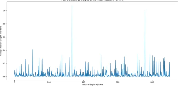
A.1.1 SVM based experiment using byte 𝑛-gram features

Figure A.15 shows a plot of raw feature weights from all overlapping time windows of size one year. Next, we computed average weights of each individual features across all time windows. The result can be seen in Figure A.16. Lastly, we computed chi-squared statistic for feature weights obtained from all time windows. This can be viewed in Figure A.17. From Figure A.17, it appears that new Vobfus variants might have been released in April 2012 time period.

(45)

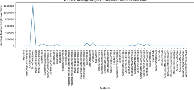
Figure A.16: Vobfus: Average weights of individual 𝑛-gram features from linear SVM.

Figure A.17: Vobfus: Chi-square Statistic.

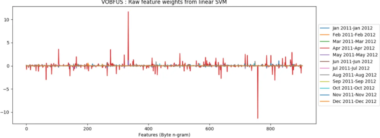
A.1.2 SVM experiment using PE file based features

For this part of experiment, linear SVM was trained using PE file based fea-tures. The result can be seen in Figure A.18, Figure A.19, and Figure A.20. From Figure A.20, it can be observed that feature weights from multiple time windows diverted significantly from their average values. From this figure it can be inferred

(46)

that variants of Vobfus undergone changes rapidly.

Figure A.18: Vobfus: Raw feature weights from linear SVM.

(47)

Figure A.20: Vobfus: Chi-square Statistic.

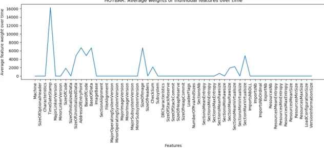
A.2 Hotbar Family

(48)

Figure A.22: Hotbar: Average weights of individual features from linear SVM.

A.3 Vbinject Family

(49)

Figure A.24: Vbinject: Average weights of individual features from linear SVM.

A.4 Winwebsec Family