On the Use of Deep Feedforward Neural Networks for Automatic Language Identification

On the use of deep feedforward neural networks for automatic

language identification

Ignacio Lopez-Moreno

a,

*

, Javier Gonzalez-Dominguez

b

, David Martinez

c

,

Oldrˇich Plchot

d

, Joaquin Gonzalez-Rodriguez

b

, Pedro J. Moreno

a

a_{Google Inc., New York, USA}

b_{ATVS-Biometric Recognition Group, Universidad Autonoma de Madrid, Madrid, Spain} c_{I3A, Zaragoza, Spain}

d_{Brno University of Technology, Brno, Czech Republic} Received 30 October 2015; accepted 18 March 2016

Available online 6 May 2016

Abstract

In this work, we present a comprehensive study on the use of deep neural networks (DNNs) for automatic language identifica-tion (LID). Motivated by the recent success of using DNNs in acoustic modeling for speech recogniidentifica-tion, we adapt DNNs to the problem of identifying the language in a given utterance from its short-term acoustic features. We propose two different DNN-based approaches. In the first one, the DNN acts as an end-to-end LID classifier, receiving as input the speech features and pro-viding as output the estimated probabilities of the target languages. In the second approach, the DNN is used to extract bottleneck features that are then used as inputs for a state-of-the-art i-vector system. Experiments are conducted in two different scenarios: the complete NIST Language Recognition Evaluation dataset 2009 (LRE’09) and a subset of the Voice of America (VOA) data from LRE’09, in which all languages have the same amount of training data. Results for both datasets demonstrate that the DNN-based systems significantly outperform a state-of-art i-vector system when dealing with short-duration utterances. Furthermore, the combination of the DNN-based and the classical i-vector system leads to additional performance improvements (up to 45% of relative improvement in both EER and Cavg on 3s and 10s conditions, respectively).

© 2016 The Authors. Published by Elsevier Ltd. This is an open access article under the CC BY license (http://creativecommons.org/ licenses/by/4.0/).

Keywords: LID; DNN; Bottleneck; i-vectors

1. Introduction

Automatic language identification (LID) refers to the process of automatically determining the language of a given speech sample (Muthusamy et al., 1994). The need for reliable LID is continuously growing due to a number of factors, including the technological trend toward increased human interaction using hands-free, voice-operated devices and the need to facilitate the coexistence of multiple different languages in an increasingly globalized world (Gonzalez-Dominguez et al., 2014).

* Corresponding author at: Google Inc, 76 Ninth Ave. P.C. 10011, New York, NY. Tel.: 9174054991. E-mail address:[email protected](I. Lopez-Moreno).

Available online atwww.sciencedirect.com

Computer Speech and Language 40 (2016) 46–59

www.elsevier.com/locate/csl

http://dx.doi.org/10.1016/j.csl.2016.03.001

0885-2308/© 2016 The Authors. Published by Elsevier Ltd. This is an open access article under the CC BY license (http://creativecommons.org/ licenses/by/4.0/).

Driven by recent developments in speaker verification, current state-of-the-art technology in acoustic LID systems involves using i-vector front-end features followed by diverse classification mechanisms that compensate for speaker and session variabilities (Brummer et al., 2012; Li et al., 2013; Sturim et al., 2011). An i-vector is a compact repre-sentation (typically from 400 to 600 dimensions) of a whole utterance, derived as a point estimate of the latent vari-able in a factor analysis model (Dehak et al., 2011; Kenny et al., 2008). While proven to be successful in a variety of scenarios, i-vector based approaches have two major drawbacks. First, i-vectors are point estimates and their robust-ness quickly degrades as the duration of the utterance decreases. Note that the shorter the utterance, the larger the variance of the posterior probability distribution of the latent variable; and thus, the larger the i-vectoruncertainty. Second, in real-time applications, most of the costs associated with i-vector computation occur after completion of the utterance, which introduces an undesirable latency.

Motivated by the prominence of deep neural networks (DNNs), which surpass the performance of the previous dominant paradigm, Gaussian mixture models (GMMs), in diverse and challenging machine learning applications – including acoustic modeling (Hinton et al., 2012; Mohamed et al., 2012), visual object recognition (Ciresan et al.), and many others (Yu and Deng, 2011) – we previously introduced a successful LID system based on DNNs in

Lopez-Moreno et al.. Unlike previous works on using neural networks for LID (Cole et al., 1989; Leena et al., 2005; Montavon, 2009), this paper represented, to the best of our knowledge, the first time a DNN scheme was applied at large scale for LID and was benchmarked against alternative state-of-the-art approaches. Evaluated using two differ-ent datasets – the NIST LRE’09 (3s task) and Google 5M LID – this scheme demonstrated significantly improved performance compared to several i-vector-based state-of-the-art systems (Lopez-Moreno et al.). This scheme has also been successfully applied as a front-end stage for real-time multilingual speech recognition, as described in (Gonzalez-Dominguez et al., 2014).

This article builds on our previous work by extensively evaluating and comparing the use of DNNs for LID with an i-vector baseline system in different scenarios. We explore the influence of several factors on the DNN architecture configuration, such as the number of layers, the importance of including the temporal context and the duration of test segments. Further, we present a hybrid approach between the DNN and the i-vector system – the

bottleneck system – in an attempt to take the best from both approaches. In this hybrid system, a DNN with a

bottleneck hidden layer (40 dimensions) acts as a new step in the feature extraction before the i-vector modeling strategy is implemented. Bottleneck features have recently been used in the context of LID (Jiang et al., 2014; Mate˘jka et al., 2014; Richardson et al.). In these previous works, the DNN models were optimized to classify the phonetic units of a specific language, following the standard approach of an acoustic model for automatic speech recognition. Unlike in these previous works, here we propose using the bottleneck features from a DNN directly optimized for language recognition. In this new approach, i) the DNN optimization criterion is coherent with the LID evaluation criterion, and ii) the DNN training process does not require using transcribed audio, which is typically much harder to acquire than language labels. Note that the transcription process involves handwork from experts that are familiarized with specific guidelines (e.g. transcriptions provided in the written domain, or the spoken domain); it is slow, as each utterance typically contains about 2 words/sec and moreover, word level transcriptions needs to be mapped into frame level alignments before a DNN such as the one used in previous works can be trained. That requires bootstrapping from another pre-existing ASR system, typically a GMM-based acoustic model iteratively trained from scratch. Instead, in the process of training lang-id networks, no previous alignments are needed, only one label per utterance is required and annotation guidelines are significantly simpler. Overall, that facilitates the adoption of a bottleneck lang-id system, which has the additional advantage that targets language discrimination in all its intermediate stages.

For this study, we conducted experiments using two different datasets: i) a subset of LRE’09 (8 languages) that comprises equal quantities of data for each target language, and ii) the full LRE’09 evaluation dataset (23 languages), which contains significantly different amounts of available data for each target language. This approach enabled us to assess the performance of all the proposed systems in cases of both controlled and uncontrolled conditions.

The rest of this paper is organized as follows:Sections 2and3present the i-vector baseline system and the archi-tecture of the DNN-based system. InSection 4, we describe the proposed bottleneck scheme. InSections 5and6, we outline fusion and calibration, and the datasets used during experimentation. Results are then presented inSection 7. Finally,Section 8summarizes final conclusions and potential future lines of this work.

2. The baseline I-vector based system 2.1. Feature extraction

The input audio to our system is segmented into windows of 25ms with 10ms overlap. 7 Mel-frequency cepstral coefficients (MFCCs), includingC0, are computed on each frame (Davis and Mermelstein, 1980). Vocal tract length normalization (VTLN) (Welling et al., 1999), cepstral mean and variance normalization, and RASTA filtering (Hermansky and Morgan, 1994) are applied on the MFCCs. Finally, shifted delta cepstra (SDC) features are computed in a 7-1-3-7 configuration (Torres-Carrasquillo et al., 2002), and a 56-dimensional vector is obtained every 10 ms by stacking the MFCCs and the SDC of the current frame. The feature sequence of each utterance is converted into a single i-vector with the i-vector system described next.

2.2. I-vector extraction

I–vectors (Dehak et al., 2011) have become a standard approach for speaker identification, and have grown in pop-ularity also for language recognition (Brummer et al., 2012; Dehak et al., 2011; Martinez et al., 2011; McCree, 2014). Apart from language and speaker identification, i–vectors have been shown to be useful also for several different clas-sification problems including emotion recognition (Xia and Liu, 2012), and intelligibility assessment (Martínez et al., 2013). An i–vector is a compact representation of a Gaussian Mixture Model (GMM) supervector (Reynolds et al., 2000), which captures most of the GMM supervectors variability. It is obtained by a Maximum–A–Posteriori (MAP) estimate of the mean of a posterior distribution (Kenny, 2007). In the i–vector framework, we model the utterance-specific supervectormas:

m= +u Tw, (1)

whereuis the UBM GMM mean supervector andTis a low-rank rectangular matrix representing the bases spanning the sub-space, which contains most of the variability in the supervector space. The i–vector is then a MAP estimate of the low-dimensional latent variablew. In our experiments, we have used a GMM containing 2048 Gaussian com-ponents with diagonal covariance matrices and the dimensionality of i-vectors was set to 600.

2.3. Classification backends

For classification, the i-vectors of each language are used to estimate a single Gaussian distribution via maximum likelihood, where the covariance matrix is shared among languages and is equal to the within-class covariance matrix of the training data. During evaluation, every new utterance is evaluated against the models of all the languages. Further details can be found in (Martinez et al., 2011).

3. The DNN-based LID system

Recent findings in the field of speech recognition have shown that significant accuracy improvements over clas-sical GMM schemes can be achieved through the use of DNNs. DNNs can be used to generate new feature repre-sentations or as final classifiers that directly estimate class posterior scores. Among the most important advantages of DNNs is their multilevel distributed representation of the model’s input data (Hinton et al., 2012). This fact makes the DNN an exponentially more compact model than GMMs. Further, DNNs do not impose assumptions on the input data distribution (Mohamed et al., 2012) and have proven successful in exploiting large amounts of data, achieving more robust models without lapsing into overtraining. All of these factors motivate the use of DNNs in language iden-tification. The rest of this section describes the architecture and practical application of our DNN system.

3.1. Architecture

The DNN system used in this work is a fully-connected feed-forward neural network with rectified linear units (ReLU) (Zeiler et al., 2013). Thus, an input at levelj,xj, is mapped to its corresponding activationyj(input of the layer above) as:

yj=ReLU x

( )

j =max

(

0,xj

)

(2)

xj bj w yij i i

= +

∑

(3)

whereiis an index over the units of the layer below andbjis the bias of the unitj.

The output layer is then configured as asoftmax, where hidden units map inputyjto a class probabilitypjin the

form: p y y j j l l =

( )

( )

∑

expexp (4)

wherelis an index over all of the target classes (languages,Fig. 2).

As a cost function for backpropagating gradients in the training stage, we use the cross-entropy function defined as:

C tj pj j

= −

∑

log ₍₅₎

wheretjrepresents the target probability of the classjfor the current evaluated example, taking a value of either 1

(true class) or 0 (false class).

3.2. Implementing DNNs for language identification

From the conceptual architecture explained above, we built a language identification system to work at the frame level as follows:

As the input of the net, we used the same features as the i-vector baseline system (56 MFCC-SDC). Specifically, the input layer was fed with 21 frames formed by stacking the current processed frame and its±10 left/right neigh-bors. Thus, the input layer comprised a total number of 1176 (21×56) visible units,v.

On top of the input layer, we stacked a total number of Nhl(4) hidden layers, each containingh(2560) units. Then,

we added the softmax layer, whose dimension (s) corresponds to the number of target languages (NL), plus one extra

output for the out-of-set (OOS) languages. This OOS class, devoted to unknown test languages, could later allow us to use the system in open-set identification scenarios.

Overall, the net was defined by a total ofwfree parameters (weights+bias), w= +

(

v 1

)

h+

(

Nhl−1

)

(

h+1

)

h+ +

(

h 1

)

s

(~23M). The complete topology of the network is depicted inFig. 1.

In terms of the training procedure, we used asynchronous stochastic gradient descent within the DistBelief frame-work (Dean et al., 2012), which uses computing clusters with thousands of machines to train large models. The learn-ing rate and minibatch size were fixed to 0.001 and 200 samples.1

Note that the presented architecture works at the frame level, meaning that each single frame (plus its correspond-ing context) is fed-forward through the network, obtaincorrespond-ing a class posterior probability for all of the target lan-guages. This fact makes the DNNs particularly suitable for real-time applications because, unlike other approaches (i.e. i-vectors), we can potentially make a decision about the language at each new frame. Indeed, at each frame, we can combine the evidence from past frames to get a single similarity score between the test utterance and the target

1_{We define sample as the input of the DNN: the feature representation of a single frame besides those from its adjacent frames forming the} context.

languages. A simple way of doing this combination is to assume that frames are independent and multiply the pos-terior estimates of the last layer. The scoreslfor languagelof a given test utterance is computed by multiplying the

output probabilitiesplobtained for all of its frames; or equivalently, accumulating the logs as:

s N p L x l l t t N =

(

)

=

∑

1 1 log ,θ (6)

where p L x

(

l t,θ

)

represents the class probability output for the languagelcorresponding to the input example at time

t,xtby using the DNN defined by parametersθ. 4. Bottleneck features: A hybrid approach

Another interesting way to leverage the discriminative power of a DNN is through the use ofbottleneck features (Fontaine et al., 1997; Grézl et al., 2009). Typically, in speech recognition, bottleneck features are extracted from a DNN trained to predict phonetic targets, by either using the estimated output probabilities (Hermansky et al., 2000) or the activations of a narrow hidden layer (Grézl et al., 2007), the so-called bottleneck layer. The bottleneck features represent a low-dimensional non-linear transformation of the input features, ready to use for further classification.

Utilizing this approach, we extracted bottleneck features from the DNN directly trained for LID, as explained in

Section 3, and replaced the last complete hidden layer with a bottleneck layer of 40 dimensions. Then, we modeled Fig. 1. Pipeline process from the waveform to the final score (left). DNN topology (middle). DNN description (right).

those new bottleneck features by using an i-vector strategy. That is, we replaced the standard MFCC-SDC features with bottleneck features as the input of our i-vector baseline system.

The underlying motivation of this hybrid architecture is to take the best from both the DNN and the i-vector system approaches. On one hand, we make use of the discriminative power of the DNN model and its capability to learn better feature representations; on the other, we are still able to leverage the generative modeling introduced by the i-vector system.

5. Fusion and calibration

We used multiclass logistic regression in order to combine and calibrate the outputs of individual LID systems (Brümmer and van Leeuwen, 2006). Let skL

( )

xi be the log-likelihood score for the recognizerkand languageLfor

utterancexi. We derive combined scores as

ˆ s xL i k kLs xi k K L

( )

=

( )

+ =

∑

α β 1 (7) Note that this is just a generic version of the product rule combination, parameterized byαandβ. Defining a multiclass logistic regression model for the class posterior as

P L s x s x s x L i L i l i l ˆ exp ˆ exp ˆ

( )

(

)

=

(

( )

( )

)

(

)

∑

(8)

we foundαandβto maximize the global log-posterior in a held-out dataset ofIutterances

Q K N tlP L s xl i l N i I L α1 α β1 β δ 1 1 ,…, , ,…

(

)

=

(

( )

)

= =

∑

∑

ˆ (9) being δiL L i w , x L , . if otherwise ∈ ⎧ ⎨ ⎩0 (10)

wherewl(l=1,…,NL) is a weight vector that normalizes the number of samples for every language in the

develop-ment set (typically, wL=1 if an equal number of samples per language is used). This fusion and calibration

proce-dure was conducted using the FoCal (Multi-class) toolkit (Brümmer).

6. Databases and evaluation metrics 6.1. Databases

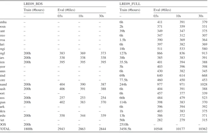
We evaluate all proposed systems in the framework of the NIST LRE 2009 (LRE’09) evaluation. The LRE’09 in-cludes data from two different audio sources: Conversational Telephone Speech (CTS) and, unlike previous LRE evalu-ations, telephone speech from broadcast news, which was used for both training and test purposes. Broadcast data were obtained via an automatic acquisition system from “Voice of America” news (VOA) that mixed telephone and non-telephone speech. Up to 2TB of 8kHz raw data containing radio broadcast speech, with corresponding language and audio source labels, were distributed to participants, and a total of 40 languages (23 target and 17 out of set) were included. While the VOA corpus contains over 2000 hours of labeled audio, only the labels from a fraction of about 200 hours were manually verified by the Linguistic Data Consortium (LDC).

Due to the large disparity in the amounts of available training material by language and type of audio source, we created two different evaluation sets from LRE’09: LRE09_FULL and LRE09_BDS. LRE09_FULL corresponds to

the original LRE’09 evaluation, which includes the original test files and all development training files for each language.2

LRE09_BDS, on the other hand, is a balanced subset of 8 languages from automatically labeled VOA audio data. While the LRE09_FULL set uses data from the manually annotated part of the VOA corpus, the LRE09_BDS con-tains audio from both automatically and manually annotated parts. This dual evaluation approach served two pur-poses: i) LRE09_FULL, which is a standard benchmark, allowed us to generate results that could be compared with those of other research groups, and ii) LRE09_BDS allowed us to conduct new experiments using a controlled and balanced dataset with more hours of data for each target language. This approach may also help identify a potentially detrimental effect on the LRE09_FULL DNN-based systems due to the lack of data in some target languages. This is important because we previously found that the relative performance of a DNN versus an i-vector system is largely dependent on the amount of available data (Lopez-Moreno et al.).

Table 1summarizes the specific training and evaluation data per language used in each dataset. 6.2. Evaluation metrics

Two different metrics were used to assess the performance of the proposed techniques. As the main error measure to evaluate the capabilities of one-vs.-all language detection, we used Cavg(average detection cost), as defined in the

LRE 2009 (Brummer, 2010; NIST, 2009) evaluation plan.Cavgis a measure of the cost of making incorrect decisions

and, therefore, considers not only the discrimination capabilities of the system, but also the ability of setting optimal thresholds (i. e., calibration). Further, the well-known metric Equal Error Rate (EER) is a calibration-insensitive metric that indicates the error rate at the operating point where the number of false alarms and the number of false rejections 2 _{We used the training dataset defined by the I3A research group (University of Zaragoza) in its participation in the LRE’11 evaluation (Martínez} et al., 2011).

Table 1

Distribution of training hours per languages and eval files in used datasets LRE09_BDS and LRE09_FULL.

LRE09_BDS LRE09_FULL

Train (#hours) Eval (#files) Train (#hours) Eval (#files)

– 03s 10s 30s – 03s 10s 30s amha – – – – 6h 411 391 379 bosn – – – – 2h 371 359 331 cant – – – – 39h 349 347 375 creo – – – – 6h 347 312 307 croa – – – – 1.5h 390 369 364 dari – – – – 6h 397 382 369 engi – – – – 18h 511 533 580 engl 200h 383 369 373 127h 866 836 913 fars 200h 338 338 338 38h 385 383 391 fren 200h 395 395 395 35.5h 401 394 388 geor – – – – 5h 403 396 398 haus – – – – 6h 430 382 345 hind – – – – 69h 640 614 668 kore – – – – 77.5h 460 450 453 mand 200h 404 390 387 244h 977 971 1028 pash 200h 406 391 388 6h 404 391 388 port – – – – 6h 457 377 339 russ 200h 257 253 254 66h 484 479 523 span 200h 402 383 370 114h 398 383 370 turk – – – – 6h 396 394 392 ukra – – – – 1h 403 383 375 urdu 200h 358 344 339 13h 386 372 371 viet – – – – 56h 282 279 315 OOS 200h – – – 2510h – – – TOTAL 1800h 2943 2863 2844 3458.5h 10548 10177 10362

are equal. Since our problem is a detection task where a binary classification is performed for each language, the final EER is the average of the EERs obtained for each language.

7. Results

In this section, we present a comprehensive set of experiments that compare and assess the two systems of inter-est, as well as a combined version of the two. Besides the i-vector-based baseline system, we evaluate the following three family of systems:

• DNNrefers to the end-to-end deep neural network based system presented inSection 3, which is used as a final classifier to predict language posteriors.

• DNN_BN: refers to an end-to-end DNN system where the last hidden layer is replaced by a bottleneck layer. This

DNN is used as a final classifier to predict language posteriors.

• BNrefers to the i-vector system where the inputs are bottleneck features, as explained inSection 4.

Individual systems vary in the number of layers used (4 or 8 layers) and the size of their input context (0, 5 or 10 left/right frames). Hereafter, we will use the family name to refer a specific system {DNN, DNN_BN, BN}, fol-lowed by a set of suffixes {4L, 8L} and the {0-0C, 5-5C, 10-10C} to denote the number of layers and input context, respectively. For instance, the system name DNN_BN_4L_5-5C refers to a DNN system with 4 layers where the last hidden layer is a bottleneck layer, which uses an input of 11 concatenated frames (5 to the left and 5 to the right of the central frame). Note that the difference between DNN_BN and BN is that in the first, the DNN with a bottleneck layer is used directly as an end-to-end classifier, while in the second the DNN is used to extract bottleneck features which are used as input to an i-vector system.

7.1. Results using LRE09_BDS 7.1.1. DNN vs i-vector system

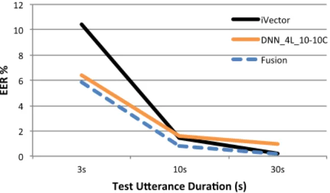
As the starting point of this study, we compare the performance of the proposed DNN architecture (with 4 layers and input context of±10 frames) and the i-vector baseline system.Fig. 3shows the difference in performance using test segments with a duration of 3s, 10s and 30s. The trend of the lines in the figure illustrates one of the main con-clusions of this work: the DNN system significantly outperforms the i-vector system for short duration utterances (3s), while the i-vector system is more robust for test utterance over 10s.

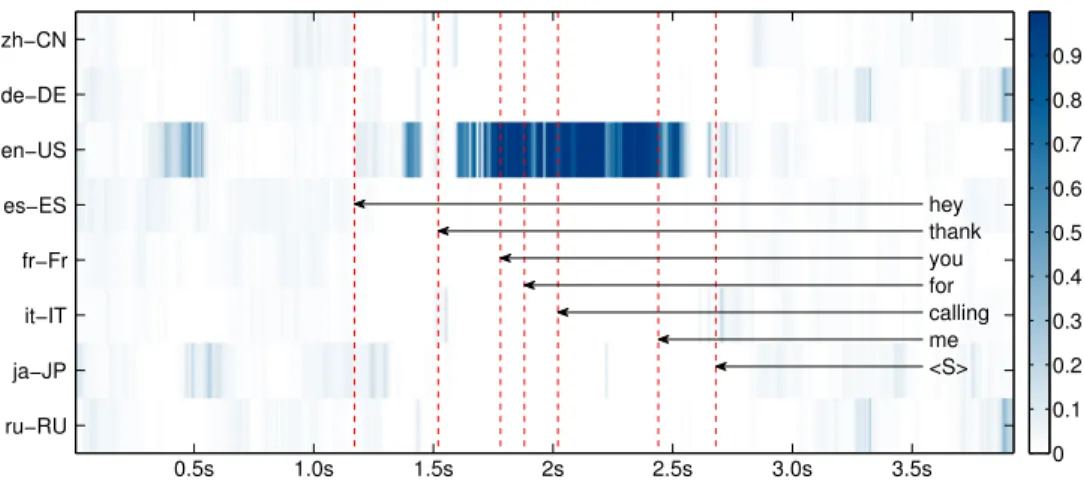
Unlike i-vectors, the DNN system does not process the complete test utterance at once. Instead, posterior scores are computed at each individual frame and combined as if each frame was independent (Eq.6). This is a frame-by-frame strategy that allows for providing continuous labels for a data stream, which may be beneficial in real time applications (Gonzalez-Dominguez et al., 2014).

7.1.2. Bottlenecks

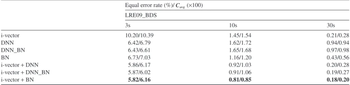
Next, we explore the use of bottleneck features in the bottleneck system. As previously stated, it is a hybrid DNN/ i-vector system where the DNN model acts as a feature extractor, whose features are used by the i-vector model instead of the standard MFCC-SDC. Specifically, we present the results of a bottleneck system that uses a DNN model with 4 layers, where the last hidden layer was replaced by a 40 dimensional bottleneck layer.Table 2compares the results from the hybrid bottleneck system with those of the standalone alternative approaches presented previously. Results show significantly improved performance for 10s and 30s utterances when using the bottleneck system (BN), as com-pared with the DNN system without bottleneck (DNN) (28% and 54% relative improvement in EER, respectively), while results for 3s utterances are similar. With respect to the i-vector, results obtained with the BN system are better in 3s and 10s (20% and 34% relative improvement in EER, respectively), whereas in 30s i-vectors still obtain better performance. Again, these results demonstrate the robustness of the i-vector system when evaluating longer test seg-ments. They also suggest that further research into this area could lead to improved results when combining the strengths of DNN and i-vector systems.

We also analyze the loss in performance of our standalone neural network system when reducing the number of nodes in the last hidden layer from 2560 (DNN system) to 40 nodes used by the DNN_BN system. That is, the DNN_BN system uses the same network that extracts the BN features, but is used as an end-to-end classifier. Results collected inTable 2show that there is not a significant difference in performance when reducing the number of nodes in the last hidden layer. This result demonstrates that bottleneck features are an accurate representation of the frame-level information; at least, comparable to that presented in the complete last hidden layer of the conventional DNN architecture. 7.1.3. Temporal context and number of layers

Another important aspect in the DNN system configuration is the temporal context of the spectral features used as the input to the DNN. Until now, we have used a fixed right/left context of±10 frames respectively. That is, the input of our network, as mentioned inSection 3, is formed by stacking the features of every frame with its corresponding 10 adjacent frames to the left and right. The motivation behind using temporal contexts with a large number of frames lies in the idea of incorporating additional high-level information into our system (i.e. phonetic, phonotactic and pro-sodic information). This idea has been widely and successfully implemented in language identification in the past, using long-term phonotactic/prosodic tokenizations (Ferrer et al., 2010; Reynolds et al., 2003) or, in acoustic ap-proaches, by using shifted-delta-cepstral features (Torres-Carrasquillo et al., 2002).

Table 3presents the performance for contextual windows of size 0, ±5 and±10 frames. Unlike the results we presented inGonzalez-Dominguez et al. (2015), where we found that the window size was critical to model the con-textual information, here just small and non-uniform gains were found. This result can be explained by the fact that, unlike the PLP features used inGonzalez-Dominguez et al. (2015), the MFCC-SDC features in this paper already include some degree of temporal information.

In addition, we evaluate the effect of increasing the number of layers to eight, doubling the number of weights in the network from 22.7M to 48.9M. The results of this evaluation are summarized inTable 3. The 8 layers topology achieved only small gains for DNN and DNN_BN in 3s segments, so we opted to keep the original 4-layer DNN as our reference DNN system.

Table 2

Performance for individual and fusion systems – average EER in % and Cavg×100– on the balanced LRE09_BDSdataset by test duration. All

DNN family systems {DNN, DNN_BN and BN} come from a DNN with 4 layers and context of±10 frames. Equal error rate (%)/Cavg(×100)

LRE09_BDS 3s 10s 30s i-vector 10.20/10.39 1.45/1.54 0.21/0.28 DNN 6.42/6.79 1.62/1.72 0.94/0.94 DNN_BN 6.43/6.61 1.65/1.68 0.97/0.98 BN 6.73/7.03 1.16/1.20 0.43/0.56 i-vector+DNN 5.86/6.17 0.92/1.03 0.20/0.28 i-vector+DNN_BN 5.87/6.02 0.91/1.06 0.19/0.27 i-vector+BN 5.82/6.16 0.81/0.85 0.18/0.20

7.1.4. Fusion and results per language

The different optimization strategies of DNN and i-vector systems (discriminative vs. generative) and the differ-ent results observed in the evaluated tasks have demonstrated the complemdiffer-entarity of these two approaches. Such complementarity suggests that further gains may be achieved through a score level combination of the systems pre-sented above, the results of which are prepre-sented in the last three rows ofTable 2. We performed a score-level com-bination of the baseline i-vector system and various neural network-based systems by means of multiclass logistic regression (Section 5). The fusion of the i-vector and bottleneck systems achieves the best performance, with relative improvements over the standalone i-vector system of 42%/40%, 44%/44% and 14%/28% in terms of EER/Cavg for

the 3s, 10s and 30s evaluated conditions, respectively. Moreover, results are consistent across all the languages and test duration conditions as shown inFig. 4. These results confirm that when bottleneck and i-vector systems are com-bined, they consistently outperform the baseline i-vector system, although the relative improvement diminishes as the test duration increases (Fig. 5).

7.2. Results using LRE09_FULL

To properly train a DNN system, we ideally need large and balanced amounts of data for each language. In this section, we evaluate the implications of having an unbalanced training dataset. Specifically, we mirror the experi-ments in the above section, instead using the entire LRE09_FULL dataset (seeTable 1for the distribution of this dataset). One of the possible approaches for dealing with an unbalanced dataset is to build a bottleneck system in the follow-ing way: First, generate a balanced subset of utterances from the most represented languages to train a network that Table 3

Performance of DNN-based systems as a function of the number of layers and temporal context used. Results on LRE09_BDS are reported as average EER on the 8 languages (%).

Equal error rate (%)

4 Layers 8 Layers 0C-0C 5C-5C 10C-10C 0C-0C 5C-5C 10C-10C 3s 10s 30s 3s 10s 30s 3s 10s 30s 3s 10s 30s 3s 10s 30s 3s 10s 30 DNN 6.8 2.00 1.07 6.66 1.64 0.95 6.42 1.62 0.94 6.90 1.94 0.98 6.40 1.72 0.92 6.23 1.61 0.94 DNN_BN 7.21 2.17 1.16 6.77 1.83 1.04 6.43 1.65 0.97 6.87 1.91 0.96 6.17 1.71 0.98 6.36 1.58 0.85 BN 7.43 1.32 0.41 7.07 1.13 0.38 6.73 1.16 0.43 9.36 2.01 0.68 8.74 1.43 0.59 9.17 1.84 0.76

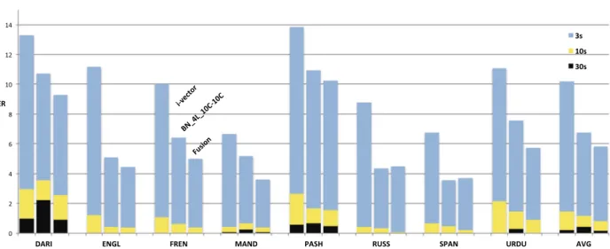
Fig. 4. i-vector, BN and fusion system performance comparison (average EER) per language on LRE09_BDS dataset. Errors bars for 30s, 10s and 3s are superimposed, and therefore, representing the actual error for every condition.

includes a bottleneck layer. This network may or may not contain all of the target languages. Then, using the previ-ous network, compute the bottleneck features from the original unbalanced dataset to optimize the remaining stages involved in the i-vector system. We simulated the unbalanced data scenario by using the eight-language DNN from

Section 7.1to compute bottleneck features over our LRE09_FULL training set. While one could consider using non-overlapping sets for the DNN and i-vector optimization to avoid overfitting, we opted to use the entire unbal-anced dataset due to data scarcity in our training material for LRE09_FULL.

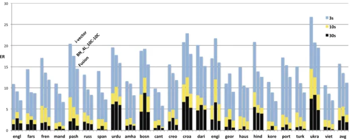
Fig. 6depicts the performance of the bottleneck system trained as explained above, the i-vector system, and their fusion, for each of the 3 conditions (3s, 10s, 30s) and the 23 target languages. The vertical line separates the perfor-mance for the languages included (left) and excluded (right) during the DNN optimization process. The results show that, despite overall good performance, the bottleneck system performs much better for the languages involved in the DNN training.

The second approach used was to train a new DNN model using all the target languages in the LRE09_FULL eval-uation. Note that, in this case, unequal amounts of training data were used to optimize each of the 23 DNN outputs. The results of this second approach are shown inFig. 7. By comparingFigs. 7 and 6, in which the only underlying difference is the training data used for the DNN model, we see that data imbalance may be an issue in the stand-alone DNN system, but it is not an issue when using the bottleneck system. Moreover, the bottleneck system seems to benefit from matching the target classes of the underlying DNN model with the target languages in the language recognition evaluation (see, for instance, the performance improvements on Georgian, Korean or Ukranian).

Fig. 5. DNN vs i-vector system performance (EER) in function of test utterance segment duration (LRE09_FULL corpus).

Fig. 6. i-vector, BN and fusion system performance comparison (average EER) per language on LRE09_FULL dataset. The DNN used to extract bottleneck features was trained just with the 8 target languages of LRE09_BDS (on the left of the vertical dashed line). Errors bars for 30s, 10s and 3s are superimposed, and therefore, representing the actual error for every condition.

Finally, the results for the LRE09_FULL dataset for all the individual systems proposed, including fusions with the baseline i-vector system, are summarized inTable 4. Note that all DNNs shown in this table were trained using data of the 23 target languages. The conclusion remains the same as in the case of the LRE09_BDS dataset (Table 2), but with modest performance improvements. Specifically, when fusing the i-vector and the bottleneck systems, we achieved improvements of 29%/27%, 32%/34% and 21%/24% in terms of EER/Cavg for the 3s, 10s and 30s

evalu-ated conditions. 8. Summary

In this work, we presented an extensive study of the use of deep neural networks for LID. Guided by the success of DNNs for acoustic modeling, we explored their capability to learn discriminative language information from speech signals.

First, we showed how a DNN directly trained to discern languages obtains significantly improved results with respect to our best i-vector system when dealing with short-duration utterances. This proposed DNN architecture is able to generate a local decision about the language spoken in every single frame. These local decisions can then be com-bined into a final decision at any point during the utterance, which makes this approach particularly suitable for real-time applications.

Next, we introduced the LID optimized bottleneck system as a hybrid approach between the proposed DNN and i-vector systems. Here, a DNN optimized to classify languages is seen as a front-end that extracts a more suitable Fig. 7. i-vector, BN and fusion systems performance comparison (average EER) per language on LRE09_FULL dataset. The DNN used to extract bottleneck features was trained with all the 23 target languages. Errors bars for 30s, 10s and 3s are superimposed, and therefore, representing the actual error for every condition.

Table 4

Performance for individual and fusion systems – average EER in % and Cavg×100 – on full LRE09_FULL dataset by test duration. All DNN family systems {DNN, DNN_BN and BN} come from a DNN with 4 layers and context of±10 frames.

Equal error rate (%)/Cavg(×100)

LRE09_FULL 03s 10s 30s i-vector 15.74/16.37 5.30/6.24 2.33/2.90 DNN_BN 13.49/14.21 6.38/7.11 4.37/4.88 BN 13.52/14.19 5.58/6.21 3.24/3.77 i-vector+DNN_BN 11.93/12.76 3.80/4.59 1.94/2.28 i-vector+BN 11.19/11.87 3.61/4.13 1.85/2.21

representation (in terms of discrimination) of feature vectors. On contrary to previous bottleneck approaches for LID, where the DNN was trained to recognize the phonetic units of a given language, in this work, the DNN optimization criterion is coherent with the LID objective. Moreover, the DNN model requires only language labels which are much easier to obtain than the speech transcriptions.

We observed that the most desirable scenario is to train the DNN with a balanced dataset that includes all the target languages. In the case of not being able to fulfill this requirement, it is preferable to include data from all target lan-guages during the DNN optimization stage, even if some lanlan-guages contain more training hours than others. In ad-dition, fusion results show that DNN-based systems provide complementary information to the baseline i-vector system. In particular, the combination of the i-vector and bottleneck systems result in a relative improvement of up to 42%/ 40%, 44%/44% and 14%/28% and 29%/27%, 32%/34% and 21%/24% for the balanced dataset LRE09_BDS and the whole LRE’09 evaluation respectively, in terms of EER/C_avgand for the 3s, 10s, and 30s test conditions.

We believe that the performance of the DNN could be improved further. In the future, we plan to experiment with other topologies/activation functions and other input features, such as filterbank energies. Further, for the sake of com-parison, in this work we chose i-vector modeling as the strategy to model the bottleneck features. It is a future line of this work to experiment with different modeling schemes that might fit better for those bottleneck features . Acknowledgment

The authors would like to thank Daniel Garcia Romero for helpful suggestions and valuable discussions. Javier Gonzalez-Dominguez worked in this project during his stay is Google supported by the Google Visitor Faculty program. This work was partly supported by the Spanish government through project TIN2011-28169-C05-02 and by the Czech Ministry of Interior project No. VG20132015129 “ZAOM” and by the Czech Ministry of Education, Youth and Sports from the National Programme of Sustainability (NPU II) project “IT4Innovations excellence in science – LQ1602”.

References

Brummer, N., 2010. Measuring, Refining and Calibrating Speaker and Language Information Extracted from Speech (Ph.D. thesis). Department of Electrical and Electronic Engineering, University of Stellenbosch.

Brummer, N., Cumani, S., Glembek, O., Karafiát, M., Matejka, P., Pesan, J., et al., 2012. Description and analysis of the Brno276 System for LRE2011. In: Proceedings of Odyssey 2012: The Speaker and Language Recognition Workshop. International Speech Communication Asso-ciation, pp. 216–223.

Brümmer, N., 2010. Fusion and calibration toolkit [software package].<http://sites.google.com/site/nikobrummer/focal>.

Brümmer, N., van Leeuwen, D., 2006. On calibration of language recognition scores. In: Proc. of Odyssey. San Juan, Puerto Rico.

Ciresan, D., Meier, U., Gambardella, L., Schmidhuber, J., 2010. Deep Big Simple Neural Nets Excel on Handwritten Digit Recognition, CoRR abs/1003.0358.

Cole, R., Inouye, J., Muthusamy, Y., Gopalakrishnan, M., 1989. Language identification with neural networks: a feasibility study. In: Communi-cations, Computers and Signal Processing, 1989. Conference Proceeding, IEEE Pacific Rim Conference on, pp. 525–529. doi:10.1109/ PACRIM.1989.48417.

Davis, S., Mermelstein, P., 1980. Comparison of parametric representations for monosyllabic word recognition in continuously spoken sentences. IEEE Trans. Acoust. Speech Signal Process. 28, 357–366.

Dean, J., Corrado, G., Monga, R., Chen, K., Devin, M., Le, Q., et al., 2012. Large scale distributed deep networks. In: Bartlett, P., Pereira, F., Burges, C., Bottou, L., Weinberger, K. (Eds.), Advances in Neural Information Processing Systems 25, pp. 1232–1240.

Dehak, N., Torres-Carrasquillo, P.A., Reynolds, D.A., Dehak, R., 2011. Language recognition via i-vectors and dimensionality reduction. In: INTERSPEECH, ISCA, pp. 857–860.

Dehak, N., Kenny, P., Dehak, R., Dumouchel, P., Ouellet, P., 2011. Front-end factor analysis for speaker verification. IEEE Trans. Audio Speech Lang. Process. 19 (4), 788–798.

Ferrer, L., Scheffer, N., Shriberg, E., 2010. A comparison of approaches for modeling prosodic features in speaker recognition. In: International Conference on Acoustics, Speech, and Signal Processing, pp. 4414–4417. doi:10.1109/ICASSP.2010.5495632.

Fontaine, V., Ris, C., Boite, J.-M., Initialis, M.S., 1997. Nonlinear discriminant analysis for improved speech recognition. In: Fifth European Con-ference on Speech Communication and Technology, EUROSPEECH 1997. Rhodes, Greece.

Gonzalez-Dominguez, J., Eustis, D., Lopez Moreno, I., Senior, A., Beaufays, F., Moreno, P., 2014. A real-time end-to-end multilingual speech recognition architecture. IEEE J. Sel. Top. Signal Process. (99), 1. doi:10.1109/JSTSP.2014.2364559.

Gonzalez-Dominguez, J., Lopez-Moreno, I., Moreno, P.J., Gonzalez-Rodriguez, J., 2015. Frame-by-frame language identification in short utter-ances using deep neural networks. Neural Netw. 64, 49–58, Special Issue on Deep Learning of Representations. doi:10.1016/j.neunet.2014.08.006. Grézl, F., Karafiát, M., Kontár, S., Cˇ ernocký, J., 2007. Probabilistic and bottle-neck features for LVCSR of meetings. In: Proc. IEEE International

Grézl, F., Karafiát, M., Burget, L., 2009. Investigation into bottle-neck features for meeting speech recognition. In: INTERSPEECH 2009, Inter-national Speech Communication Association, pp. 2947–2950.

Hermansky, H., Morgan, N., 1994. RASTA processing of speech. IEEE Trans. Speech Audio Process. 2 (4), 578–589.

Hermansky, H., Ellis, D.P.W., Sharma, S., 2000. Tandem connectionist feature extraction for conventional HMM systems. In: PROC. ICASSP, pp. 1635–1638.

Hinton, G., Deng, L., Yu, D., Dahl, G., Mohamed, A., Jaitly, N., et al., 2012. Deep neural networks for acoustic modeling in speech recognition: the shared views of four research groups. IEEE Signal Process. Mag. 29 (6), 82–97. doi:10.1109/MSP.2012.2205597.

Jiang, B., Song, Y., Wei, S., Liu, J.H., McLoughlin, I.V., Dai, L.-R., 2014. Deep bottleneck features for spoken language identification. PLoS ONE 9 (7), e100795. doi:10.1371/journal.pone.0100795.

Kenny, P., 2007. Joint factor analysis of speaker and session variability: theory and algorithms.<http://www.crim.ca/perso/patrick.kenny/FAtheory.pdf>.

Kenny, P., Oullet, P., Dehak, V., Gupta, N., Dumouchel, P., 2008. A study of interspeaker variability in speaker verification. IEEE Trans. Audio Speech Lang. Process. 16 (5), 980–988.

Leena, M., Srinivasa Rao, K., Yegnanarayana, B., 2005. Neural network classifiers for language identification using phonotactic and prosodic fea-tures. In: Intelligent Sensing and Information Processing, 2005. Proceedings of 2005 International Conference on, pp. 404–408. doi:10.1109/ ICISIP.2005.1529486.

Li, H., Ma, B., Lee, K.A., 2013. Spoken language recognition: from fundamentals to practice. P. IEEE 101 (5), 1136–1159. doi:10.1109/ JPROC.2012.2237151.

Lopez-Moreno, I., Gonzalez-Dominguez, J., Plchot, O., Martinez, D., Gonzalez-Rodriguez, J., Moreno, P., 2014. Automatic language identifica-tion using deep neural networks. Acoustics, Speech, and Signal Processing, IEEE Internaidentifica-tional Conference on.

Martínez, D., Villalba, J., Ortega, A., Lleida, E., 2011. I3A language recognition system description for NIST LRE 2011. In: NIST 2011 LRE Work-shop Booklet. Atlanta, Georgia, USA.

Martínez, D., Green, P.D., Christensen, H., 2013. Dysarthria intelligibility assessment in a factor analysis total variability space. In: INTERSPEECH 2013, 14th Annual Conference of the International Speech Communication Association. Lyon, France, pp. 2133–2137. August 25–29. Martinez, D., Plchot, O., Burget, L., Glembek, O., Matejka, P., 2011. Language recognition in iVectors space. In: INTERSPEECH. ISCA, pp. 861–

864.

Mate˘jka, P., Zhang, L., Ng, T., Mallidi, H.S., Glembek, O., Ma, J., et al., 2014. Neural network bottleneck features for language identification. In: Speaker Odyssey, pp. 299–304.

McCree, A., 2014. Multiclass discriminative training of i-vector language recognition. In: IEEE Odyssey: The Speaker and Language Recognition Workshop. Joensu, Finland.

Mohamed, A., Dahl, G., Hinton, G., 2012. Acoustic modeling using deep belief networks. IEEE Trans. Audio Speech Lang. Process. 20 (1), 14– 22. doi:10.1109/TASL.2011.2109382.

Mohamed, A.-R., Hinton, G.E., Penn, G., 2012. Understanding how deep belief networks perform acoustic modelling. In: ICASSP. IEEE, pp. 4273– 4276.

Montavon, G., 2009. Deep learning for spoken language identification. In: NIPS Workshop on Deep Learning for Speech Recognition and Related Applications.

Muthusamy, Y., Barnard, E., Cole, R., 1994. Reviewing automatic language identification. IEEE Signal Process. Mag. 11 (4), 33–41. doi:10.1109/ 79.317925.

NIST, 2009. The 2009 NIST SLR Evaluation Plan.<www.itl.nist.gov/iad/mig/tests/lre/2009/LRE09_EvalPlan_v6.pdf>.

Reynolds, D., Quatieri, T., Dunn, R., 2000. Speaker verification using adapted Gaussian mixture models. Dig. Sig. Process. 10 (1/2/3), 19–41. Reynolds, D., Andrews, W., Campbell, J., Navratil, J., Peskin, B., Adami, A., et al., 2003. The SuperSID project: exploiting high-level

informa-tion for high-accuracy speaker recogniinforma-tion. In: IEEE Internainforma-tional Conference on Acoustics, Speech, and Signal Processing, vol. 4, pp. 784– 787.

Richardson, F., Reynolds, D., Dehak, N., 2015. A Unified Deep Neural Network for Speaker and Language Recognition arXiv:1504.00923.

<http://arxiv.org/abs/1504.00923>.

Sturim, D., Campbell, W., Dehak, N., Karam, Z., McCree, A., Reynolds, D., et al., 2011. The MIT LL 2010 speaker recognition evaluation system: scalable language-independent speaker recognition. In: Acoustics, Speech and Signal Processing (ICASSP), 2011 IEEE International Confer-ence on, pp. 5272–5275. doi:10.1109/ICASSP.2011.5947547.

Torres-Carrasquillo, P.A., Singer, E., Kohler, M.A., Deller, J.R., 2002. Approaches to language identification using Gaussian mixture models and shifted delta cepstral features. In: ICSLP, vol. 1, pp. 89–92.

Welling, L., Kanthak, S., Ney, H., 1999. Improved methods for vocal tract normalization. In: Proceedings of the 1999 IEEE International Con-ference on Acoustics, Speech, and Signal Processing, ICASSP ‘99. Phoenix, Arizona, USA, pp. 761–764. March 15–19.

Xia, R., Liu, Y., 2012. Using i-vector space model for emotion recognition. In: INTERSPEECH 2012, 13th Annual Conference of the Interna-tional Speech Communication Association. Portland, Oregon, USA, pp. 2230–2233. September 9–13.

Yu, D., Deng, L., 2011. Deep learning and its applications to signal and information processing [exploratory DSP]. IEEE Signal Process. Mag. 28 (1), 145–154. doi:10.1109/MSP.2010.939038.

Zeiler, M., Ranzato, M., Monga, R., Mao, M., Yang, K., Le, Q., et al., 2013. On rectified linear units for speech processing. In: 38th International Conference on Acoustics, Speech and Signal Processing (ICASSP). Vancouver.