An accelerated Branch-and-Bound algorithm for assignment problems of utility systems

An accelerated Branch-and-Bound algorithm for assignment

problems of utility systems

Alexandros M. Strouvalis

_{, Istvan Heckl}

_{, Ferenc Friedler}

_{, Antonis C. Kokossis}

_*

b_{Department of Computer Science,Uni6ersity of Veszpre´m,Egyetem u.10,Veszpre´m H-8200,Hungary}

c_{Department of Chemical and Process Engineering,School of Engineering in the En6ironment,Uni6ersity of Surrey,Guildford GU2 7XH,UK}

Abstract

A methodology is proposed for implementing logic and engineering knowledge within a Branch-and-Bound algorithm and with a purpose to accelerate convergence. The development addresses assignment problems of utility networks with an emphasis on the optimal allocation of units for maintenance problems. Proposed criteria are presented to automatically tailor the solution strategy and fully customise the optimisation solver. Model and problem properties are exploited to reduce the solution space, prioritise the branching of nodes, calculate lower bounds, and prune inferior parts of the binary tree. Comparisons with commercial MILP solvers demonstrate the significant merits of customising the solution search engine to the particular solution space. Extraction of knowledge and analysis of operations is conceptually supported by the graphical environment of the Hardware Composites. © 2002 Published by Elsevier Science Ltd.

Keywords:Turbine networks; Maintenance scheduling; Operational planning; MILP solvers; Hardware composites

www.elsevier.com/locate/compchemeng

1. Introduction

The impact of Mathematical Programming proves significant through a wide range of applications. Opera-tions Research groups developed and contributed con-siderable part of the available optimisation tools. At their best, they epitomise general theoretical, computa-tional and numerical knowledge in relevance to the different classes of problems. Past methods have proved unable to capture application features automatically. In the absence of specific knowledge, the use of general-purpose heuristics remains the only venue to accelerate

the search and/or reduce the solution space.

Consider-ing that optimisation technology is a natural extension of simulation — now widely accepted in industry — it might be instructive to recall that simulation earned acceptance and credit only with the use of customised algorithms (c.f. the inside-out algorithm for distilla-tion). In a similar vane, optimisation solvers should make an effort to systematically incorporate problem

information. In the case of MILP’s, the efficiency of a Branch-and-Bound algorithm is affected by the node branching criteria (Geoffrion & Marsten, 1972; Parker & Rardin, 1988; Floudas, 1995). In the absence of specific knowledge, the use of general search rules can not guarantee performance tantamount to the difficulty or the actual size of the problem.

A first major contribution to exploit problem logic involved the modelling stage. Floudas and Grossmann (1995) reviewed methods for reducing the combinato-rial complexity of discrete problems using logic-based models. Raman and Grossmann (1992) reported im-provements in solving MINLP’s with a combined use of logic and heuristics. They illustrated their ideas with inference logic for the branching of the decision vari-ables (1993), and studied the use of logical disjunctions as mixed-integer constraints (1994). Turkay and Gross-mann (1996) extended the application of logic disjunc-tions to MINLP’s using logic-based versions of OA and GBD algorithms. Hooker, Yan, Grossmann and Ra-man (1994) applied logic cuts to decrease the number of nodes in MILP process networks models. Friedler, Tarjan, Huang and Fan (1992) illustrated the potential for dramatic reductions in the solution space. Friedler,

* Corresponding author. Tel.: +44-1483-300800; fax: + 44-1483-686581.

E-mail address:[email protected](A.C. Kokossis).

0098-1354/02/$ - see front matter © 2002 Published by Elsevier Science Ltd. PII: S 0 0 9 8 - 1 3 5 4 ( 0 1 ) 0 0 7 8 8 - 8

Varga and Fan (1995) later introduced a decision map-ping approach that is particularly efficient for process

synthesis applications. Vecchietti and Grossmann

(1999) discussed the development of a solver (LOG-MIP) for solving disjunctive, algebraic MINLP or hy-brid non-linear optimisation problems. They later, (2000) presented a modelling language to set up the disjunctions and logical constraints. Lee and Gross-mann (2000) proposed a non-linear relaxation of the Generalised Disjunctive Programming and developed a special Branch-and-Bound algorithm that makes use of information of the relaxed problem to decide on the branching of terms of disjunctions.

The present work explains the integration of knowl-edge at a more advanced level: the solution search engine. The problem structure is exploited to prioritise and co-ordinate the optimisation search. A Customised Branch-and-Bound Solver (B&B) is developed to incor-porate conceptual information. The approach reports significant reductions in the computational effort and supplements the work of Strouvalis, Heckl, Friedler and Kokossis (2000). The methodology makes use of

Hardware Composites, (Mavromatis & Kokossis,

1998a,b,c; Strouvalis, Mavromatis & Kokossis, 1998). The tool supports the customisation of the algorithm, provides insights of utility operations and promotes the understanding of results.

2. Assignment problems and optimisation challenges

The problem taken into account deals with the as-signment of units to shut-down periods. The appropri-ate sequence of switching off turbines and boilers for preventive maintenance contributes to the reliability, availability and profitability of the entire system. Each period relates to either a single or multiple sets of constant demands in power and process heat. Optimal scheduling assumes meeting demands and maintenance needs while minimising the operational cost. Switching off units imposes penalties to the economic perfor-mance of the network. As less efficient units are loaded or power is purchased from grid to compensate for the ones maintained, optimisation has to consider demand variations over time, differences in the efficiencies of units and feasibility aspects.

Formulations yield MILP problems with a consider-able number of variconsider-ables. Constraints are linear and

binary variables are assigned for the ON/OFF status of

units. Planning and Scheduling Problems of large-scale networks are computationally expensive or even in-tractable. This is due to the exponential growth of combinatorial load with the number of periods and units. Conventional approaches suggest the formulation of efficient models solved by standard commercial opti-misation platforms. Even for moderate networks,

how-ever, the problem assumes prohibitive dimensions. Furthermore, due to minor differences in nearby solu-tions, the Branch-and-Bound trees are generally flat and difficult to fathom. General-purpose solvers are unable to capitalise on available information out of the general-purpose tuning, bounding and pruning frame-work they employ. Therefore, there is scope for efficient

optimisation tools customised to the particular

application.

3. Development of the Branch-and-Bound algorithm

The problem domain consists of three major compo-nents: utility network, demands, and maintenance re-quirements. Efficiencies and layout of units, operational costs, and constraints set up the network component. The fluctuating pattern of demands is a parameter of the problem along with the maintenance needs of each turbine and boiler. The problem domain is researched to define and prioritise the solution space and thus customise the algorithm. Conceptual analysis, feasibil-ity assessment of maintenance scenarios, and cost as-sessment of basic maintenance scenarios are employed to preprocess the space. Conceptual analysis is achieved by plotting demands on the Hardware Composites and understanding the role of units over time. A set of LP’s are solved to find infeasible options and objective func-tion values of modes corresponding to the shut-down of individual units in all possible periods.

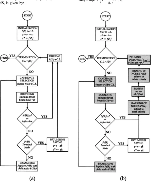
A standard B&B algorithm (i.e. Dakin, 1965; Flou-das, 1995) is shown in Fig. 1(a) and consists of six major steps: (i) initialisation, (ii) termination, (iii) selec-tion of candidate subproblem, (iv) relaxaselec-tion (bound-ing), (v) pruning and (vi) separation (branching). The proposed customisation spans over the four main stages (highlighted boxes in Fig. 1(b)): candidate problem selection, bounding, branching and pruning. Special additional functions identify (mark) and exclude (delete) inferior nodes that should not be enumerated.

The contributions are at two levels.

(i) The conceptual analysis of the problem and the assignment of priorities (period and unit).

(ii) The tuning and customisation of the solver to the particular application.

The reduction of the solution space is accomplished by screening out infeasible and redundant combinations of variables. This first level makes simple and straight-forward use of the engineering information and is re-ferred as the Preprocessing Stage. The second level constitutes a more refined analysis of the knowledge. The basic idea is to replace general B&B rules by a number of criteria and functions to co-ordinate the branching and enhance the pruning.

3.1. Solution space preprocessing

3.1.1. Conceptual tools

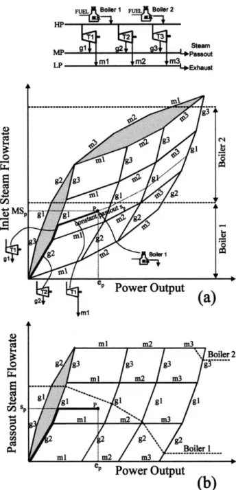
The Hardware Composites have been developed for representing the feasible and optimal space of steam turbine networks. Visualised solution spaces function as ‘maps’ where demands are traced and corresponding turbine modes identified. The tool is based on the well-established Willans line (Church, 1950; Kearton, 1958) which models the expansion of steam through cylinders. For a single turbine t (Fig. 2(a)), inlet steam

flowrate MSt is given by:

MSt=mtE+ct (1)

whereEis the turbine power output,mtthe slope of the

line associated with the expansion path efficiency andct

the no-load constant. Feasible modes locate on the Willans line.

For a backpressure passout turbine (Fig. 2(b)) the second cylinder gives rise to an additional term ac-counting for the passout flowrate and the associated power generation. The inlet steam consumption is given by the equation:

MSt=mtE+

gt

Fig. 2. Willans lines for (a) single and (b) backpressure passout turbines.

An alternative and equivalent representation is shown in Fig. 3(b); the Hardware Composites are drawn with the power and passout steam as co-ordi-nates. This version allows for directly spotting sets of demands on the solution space and is mainly adopted in the present work.

3.1.2. Assignment of priorities

The relative position of the demands and the units on the Hardware Composites determines favourable, unfa-vourable and impossible maintenance combinations. As units are switched off, the penalties imposed to the

Fig. 3. Alternative Hardware Composites representations: (a) inlet steam vs. power output and (b) passout steam vs. power output.

whereSstands for the steam passout demand andgtis

the Willans line slope associated with the high-pressure expansion path. A turbine capability diagram may be restrained by lines rt=(1−mt/gt) and pt=1/(1/mt−1/

gt) corresponding to power and inlet steam capacities,

respectively. Feasible operational modes are all inside the capability diagram. Operation of boilers and gas turbines is similarly defined by linear models presented in Appendix A.

The application of Construction Rules of Mavroma-tis and Kokossis (1998b) resolves efficiency conflicts and structures the optimal solution space of the entire turbine network. The rules impose full loading of the most efficient expansion paths prior to less efficient

ones. Slopes m and g (incremental efficiencies) of the

Willans lines define the line sequence on the Hardware Composites. Objective is minimisation of the inlet steam consumption, or equivalently the cost of fuel burnt in the boiler house.

Given the efficiencies and capacities of turbines (ca-pability diagrams) and boilers, the Hardware Com-posites of a network featuring three steam turbines and two boilers are shown in Fig. 3(a). Any point on the Composites corresponds to unique set of demands and

optimal mode. P, for example, designates the network

operation for meeting powerepand passoutspdemands

with the least steam requirement MSp. The path from

the graph origin to Preveals the load of cylinders and

depicts the role of units. The high-pressure cylinders of

T2(at full load) andT1(supplementary) supply passout

sp. The T1 low-pressure cylinder generates the

remain-ing power output requirement ofP. Dashed zones over

the Hardware Composites denote operation of boilers and their steam generation capacities. Less fuel-con-suming boilers first switch on to meet turbine inlet steam requirements. For greater flowrates (upper-right part of solution space) additional boilers accommodate

the demands. AtP, inlet steam MSpis entirely provided

objective function vary with the (i) unit efficiency, (ii) the efficiency of the units available to replace them and (iii) the demands of the particular period. Each period is affected to a different extent and priorities are strong functions of the layout of demands. High priorities for maintenance options relate to minor alterations in the operation of the utility network. Conceptual analysis (Strouvalis et al. (2000)), based on the Hardware Com-posites, provides knowledge and insights of the space and prioritises maintenance options.

In addition to conceptual preprocessing, priorities are established computationally as well for the sake of

automation. Associated with each periodtTare lower

bounds corresponding to the (lowest) operating cost (objective function) that employs all units uU. Let the set of lower bounds, Costoper_={c

T_t}, over all periodsn

of the time horizon be: Costoper_={c

T_tt=1, …,n} (3)

For an idle u in period k a penalty p(u, Tk) is

assigned calculated by shutting down exactly u and

evaluating the new objective value,CuT_k. The penalty is

given by:

p(u,Tk)=(CuT_k−cT_k) (4)

Let OSupenbe the ordered set of penalties in ascending

order:

OSupen={(CuT_t−cT_t)uU,tT} (5)

Let OSuperdefine the prioritised periods forufrom the

penalty sequence in OSupen:

OSuper={Tu i_{i=1, …,n} (6)} where: Tu1=Tt(CuT_t−cT_t)=min tT OSu pen ₍₇₎

Period Tu1 has the highest priority, followed in OSuper

by periods of decreasing priority. The periods for each

u in OSuper are alternatively represented as Tuk(u); Tu1

corresponds to k(u)=1, Tu2 to k(u)=2, etc.

Priorities over units are developed by calculating arithmetic averages Puaver over the first N(u) entries of

the OSupen. N(u) is defined by the following heuristic:

Let:

a=NT

A (8)

(non-integer values are rounded to previous integer,

with a]1))

b(u)=number of periods in OSuper (9)

N(u)=min{a,b(u)} (10)

Ais the weight parameter associated with the length of

operating horizon.

The firstN(u) penalties of OSupenare used to provide

the arithmetic average Puaver: Puaver= 1 N(u) % N(u) n=1 p(u,Tun) (11)

PenaltiesPuaverfor unitsu sorted in descending order

provide ordered set OSU:

OSU={ui:Puaver_i ]Puaver_j ,Öj\i} (12)

Let us represent the integer solution space by a

matrix with rows SMRi that correspond to units and

columns SMCj that relate to periods. The elements of

the matrix are binary variables allocating maintenance periods. The prioritisation of periods and units (OSuper

and OSU) defines the sequences SMRiover the columns

and rows, respectively. The Solver Matrix of the solu-tion space is thus obtained by:

SMRi=OSuper_j :rank(OSU,uj)=i (13)

Rows follow the sequence of units in OSU with

periods ordered according to OSuper per row.

3.2. Tuning of the sol6er

3.2.1. Customised branching

Established priorities for periods and units encom-pass the knowledge of the particular utility network and variation of demands. Let us consider as Candidate List (CL) the running list of candidates for enumera-tion. The list includes nodesw=(Tu₁

k(u1)

,Tu₂ k(u2)

, …,Tu_n k(un)₎

that define specific subproblems (combination of binary

variables assigning shut-down of units). Period Tu₁

k(u1)

corresponds to the maintenance of the first unit of OSU[Yu₁Tu₁

k(u1)

=0], Tu₂ k(u2)

is the maintenance period of

u2[Yu₂Tu₂ k(u2)

=0], etc. If a node does not involve a

decision for the maintenance of a unit, symbol (X)

defines the corresponding relaxation. In the customised

solver (X) represents the exclusion of the maintenance

requirements (constraints) of u at the specific

enumer-ated node. Parent nodewo=(X,X, …,X) represents the

relaxed subproblem where no unit maintenance is as-signed to any period. Node (Tu₁

k(u1)

,Tu₂ k(u2)

,X, …,X) rep-resents the relaxed subproblem where the first two units in priority are allocated to maintenance periods with the rest assigned to no period. The bound value of node

wis represented by B(w). Assume node w=(Tu₁ k(u1) ,Tu₂ k(u2) , …,Tu_m k(um) ,X, …,X)

with the units in priority list OSUup tomswitched off

in periods Tu₁ k(u1)_,T u₂ k(u2)_{, …,T} u_m k(um)_{, respectively.} “ IfTu₁ k(u1)_"T u₂ k(u2)_"…"T u_m

k(um)_{, node w is called}

inde-pendent. An independent node includes independent periods.

“ If at least two out of periodsTu₁ k(u₁)

,Tu₂ k(u₂)

, …,Tu_m k(u_m)

are identical, nodewis called dependent. The

“ If node w is infeasible, it is classified as dependent with infinite bound.

Based on the properties of dependent and indepen-dent nodes, bounds are determined by penalty values

p(un,Tu_n

k(un)_{) according to the following Lemma.}

Lemma. Let a parent node:

w=(Tu₁ k(u₁) ,Tu₂ k(u₂) , …,Tu_m k(u_m) ,X, …,X)

and a child node:

w%=(Tu₁ k(u1)_,T u₂ k(u2)_{, …,T} u_m k(um)_,T u_n k(un)_{,X, …,X)}

(i) if w% is independent then B(w%)=B(w)+p(un,Tu_n

k(un)_{) (14)}

(ii) if w% is dependent then B(w%)]B(w)+p(un,Tu_n k(un)_{) (15)} If node wis terminal: B(w)=B(w0)+ % U_M i=1 p(ui,Tu_i k(ui)_{) (}w _{independent) (16)} B(w)]B(w0)+ % UM i=1 p(ui,Tu_i k(u_i) ) (w dependent) (17)

where UM is the total number of units subject to mainte -nance and w0=(X, X, …, X).

Branching of nodes is handled by two criteria: the Branching Variable Selection [BVSC] and Candidate Problem Selection Criterion [CPSC]. The scope of [BVSC] is to define the membership of CL and the ordering of the subproblems in it. The [CPSC] is re-sponsible for executing the enumeration of the next node from the ones included in CL.

3.2.1.1. Branching 6ariable selection criterion [BVSC]. The [BVSC] determines (i) the membership in the CL and (ii) the ordering of nodes in CL. This criterion uses sets OSU and OSuper.

3.2.1.2. Candidate problem-node selection criterion

[CPSC]. The Candidate Problem Selection Criterion

[CPSC] has the task to select the next node for branch-ing out of the CL of nodes. The criterion adopts a Depth-First strategy with backtracking; the Last-In-First-Out (LIFO) selects a child from parent node, whereby, the last added to CL is the first one to select. When a child node is pruned, backtracking of the parent node identifies other child nodes not yet enumer-ated. The (LIFO) criterion is chosen on the merits of requiring less candidate storage and calculation restarts than the Best-Bound alternative, as Parker and Rardin (1988) mention. The (LIFO) strategy implemented in a

standard B&B, however, involves the solution of greater numbers of candidate subproblems. The cus-tomised pruning and bounding eliminate a significant portion of the explicitly visited nodes and overcome this drawback.

3.2.2. Customised pruning

Standard pruning disregards nodes with higher bounds (Fig. 1(a)). The proposed enhanced pruning consists of two additional criteria: (i) Mark and (ii) Delete Criterion (Fig. 1(b)). The first ‘marks’ subprob-lems in relation to dependent nodes, while the second eliminates from CL the qualified for pruning nodes.

Enhanced pruning exploits the properties of depen-dent and independepen-dent nodes. The methodology makes

use of sets OSuper to select combinations and exclude

redundant enumerations; nodes that follow independent nodes are pruned. For dependent nodes further branch-ing is required.

3.2.2.1.Mark criterion[MC]. The Mark Criterion [MC] imposes the enumeration of nodes due to conflicts in

priorities. [MC] applies on any node w retrieved from

the CL. For a general dependent node w=

(Tu₁ k(u₁) , …,Tu_n k(u_n) ,X, …,X), where periods Tu₁ k(u₁) Tu_n k(u_n)

, [MC] marks the nodes w1=(Tu₁ k(u₁)+1 ,X, …,X), andw2=(Tu₁ k(u₁) , …,Tu_n k(u_n)+1 ,X, …,X) for enumeration. The number of marked nodes equals the number of dependent periods present in the dependent node. The same procedure is applied to units and periods of infeasible nodes.

3.2.2.2. Delete criterion [DC]. The Delete Criterion is applied on terminal or pruned nodes and it removes from CL unmarked nodes. [DC] eliminates nodes start-ing from the end of the CL up to the point a marked node is found. The elimination then halts and enumera-tion of marked nodes is enforced. If no marked node is present [DC] eliminates the entire list.

3.2.2.3. Theorems of customised pruning. Nodes w% qualified for enhanced pruning are defined by Theorem 1 and Theorem 2. The first defines pruned subproblems associated to independent nodes while the second to dependent ones.

Theorem 1.Let a terminal independent node:

w1=(Tu₁ k(u1) ,Tu₂ k(u2) , …,Tu_n k(un)₎ or a pruned independent node:

w2=(Tu₁ k(u1)_,T u₂ k(u2)_{, …,T} u_n k(un)_{,X, …,X)} For e6ery node:

w%1=(Tu₁ k%(u₁) ,Tu₂ k%(u₂) , …,Tu_n k%(u_n) ) or

w%2=(Tu₁ k%(u1) ,Tu₂ k%(u2) , …,Tu_n k%(u_n) ,X, …,X) with k%(ui)]k(ui), Öi{1, …,n}it holds: B(w1)5B(w%1) and B(w2)5B(w%2) (18) Theorem 2. Let Tu_k k(uk)_T u_j k(uj) _{on a terminal dependent} node: w1=(Tu₁ k(u1) ,Tu₂ k(u2) , …,Tu_k k(uk) , …,Tu_j k(uj)_{, …,T} u_n k(un) )

or a pruned dependent node:

w2=(Tu₁ k(u1) ,Tu₂ k(u2) , …,Tu_k k(uk) , …,Tu_j k(uj)_{,X, …,X)} For e6ery node:

w%1=(Tu₁ k%(u1) ,Tu₂ k%(u2) , …,Tu_k k(uk) , …,Tu_j k(uj)_{, …,T} u_n k%(un)₎ or w%2=(Tu₁ k%(u1) ,Tu₂ k%(u2) , …,Tu_k k(uk) , …,Tu_j k(uj)_{,X, …,X)} with k%(ui)]k(ui), Öi{1, …,n}it holds: B(w1)5B(w%1) and B(w2)5B(w%2) (19)

Proofs of Theorem 1 and Theorem 2 are presented in Appendix B.

3.2.3. Customised bounding

The accelerated algorithm bounds nodes by capitalis-ing on information of the Preprocesscapitalis-ing Stage. Rather than calling the LP solver in every node for estimation of bounds (by fixing branched variables to integer values and relaxing the remaining ones), a more refined policy of solving LP’s is adopted. Independent node combinations relate to decoupled maintenance (mainte-nance of units in non-identical periods). These nodes are appropriate for having their bounds defined by already available values. Nodes, on the contrary, asso-ciated to coupled combinations need separate bounding and LP solution. As such the intelligent and restrained use of the LP solver reduces the resources spent on bounding.

The approach includes: 1. Selective processing of nodes, 2. Selective processing of constraints.

3.2.3.1. Selecti6e processing of nodes. Customised bounding applies only to independent nodes. In this case the solution of separate LP’s to develop bounds becomes redundant. Indeed, bounding only requires updates of bounds through straightforward calcula-tions. The approach makes use of the penalty values

p(ui,Tu_i k(u_i)

) to define the bound increase during branch-ing. For dependent nodes, bounds follow conventional

procedures. These nodes are bounded using the LP solver.

Overall, bounding makes a restricted use of the LP solver. The tightness of bounds is though relaxed, be-cause, some of the maintenance constraints are disre-garded; i.e. for the bound ofw1=(T1,X), maintenance

constraints of the second unit are not considered. As the remaining (relaxed) maintenance constraints are not taken under consideration less tight lower bounds are obtained.

3.2.3.2.Selecti6e processing of constraints. Development of customised bounds is a combined application of a customised use of the LP solver and preprocessing information. In that perspective every subproblem must be examined disregarding all maintenance constraints of child nodes. This allows for decoupling decisions-constraints between parent and child nodes or equiva-lently between periods. In that manner calculation of bounds is permitted using values of the preprocessing. The LP solver addresses subproblems where all bi-nary variables are set to fixed values. Maintenance constraints coupling periods are introduced at each branching level. Nodes not already branched have the corresponding unit maintenance constraints (and hence binary variables) excluded from the bound calculation of their parent nodes. This allows the examination of decoupled scenarios using already available bounds. Only coupled operations, where shut-down of units affects more than one periods, are examined by sepa-rate LP’s.

4. Implementation

The customised Branch-and-Bound solver is

imple-mented in C+ + and uses LINX (Fabian, 1992) as the

LP solver.LINXis a simplex-based routine collection to

facilitate special-purpose solvers and support the suc-cessive use of LP’s in relevant sub-problems. The B&B solver features options for the implemented level of customisation. Options account for conventional B&B pruning or pruning based on [DC] and [MC]. As usual, priorities can alternatively be set by users.

5. Illustration

5.1. Problem description

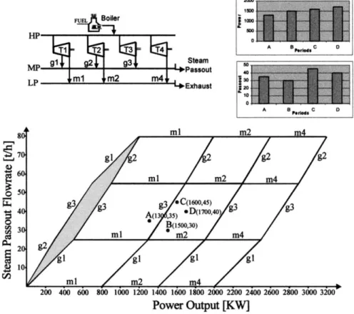
The problem considers four steam turbines with the efficiencies of Table A1 (Appendix A). The time hori-zon consists of four time periods. Maintenance requires one shut-down period per unit. Sets of data in power

and heat (A, B, C, D) are plotted on the Hardware

Fig. 4. The utility network and the hardware composites for illustration.

Step I: Preprocessing of Solution Space (i) Preliminary Reduction of Solution Space

The sets of maintenance periods are:

M(TU₁)={A,B,C}

M(TU2)={A,B,C,D} M(TU₃)={A,B,C,D}

M(TU4)={A,B,C,D}

Operation of turbine TU₁is compulsory in D due

to the high power demand. The large capacity of

TU₁ safeguards the feasible operation and

ex-cludes period D from the set of possible mainte-nance periodsM(TU1) of TU1.

(ii) Period prioritisation: ValuescT_tare calculated for

eachTt and shown in Table 1:

Solution of 4×4=16 LP’s yields the operational

costs CuT_t of Table 2.Penalties p(u,Tt)=

(CuT_t−CT_t) are then defined (each considering

one unit off) as shown in Table 3:Sorted in as-cending order penalties p(u, Tt) determine sets

OSupen: OSTUpen₁={4433.3, 6022.2, 6388.9} OSTUpen₂={0, 222.2, 888.9, 1333.3} OSTUpen₃={55.6, 83.3, 166.6, 222.2} OS_TU 4 pen_{={0, 0, 0, 0}}

Next, associated periods Tt to penalties of OSupen

provide the priority lists OSuper:

OSTUper₁={A,C,B}

OSTUper₂={A,C,B,D}

OSTUper₃={B,A,D,C}

OSTUper₄={D,C,B,A} Table 1

Minimum operational costcT_t perTtfor illustration Period

A B C D

26 666.7 cTt($/period) 21 666.7 21 111.1 27 777.8

Table 2

Operational costs ($/period) of maintenance scenarios for illustration Period D A B C Infeasible TU1 26 100 27 500 33 800 21 666.7 22 000 TU2 28 000 28 000 26 833.3 28 000 2166.7 TU3 21 750 21 666.7 21 111.1 27 777.8 26 666.7 TU4

Table 3

Penalties ($/period) of maintenance scenarios for illustration Period B C A D TU1 4433.3 6388.9 6022.2 – TU2 0 888.9 222.2 1333.3 55.6 222.2 83.3 166.6 TU3 0 TU4 0 0 0

less differently stated (dependent nodes), all lower bounds are calculated by adding to the lower bound of the parent node the penalty for shutting down a unit (associated to the branching level) in a specific period. The B&B tree and the branching of nodes are pre-sented in Fig. 5. Node numbers reflect the branching sequence. Information is also given for bound and penalty values.

The optimum maintenance vector is:

(TU1, TU3, TU2, TU4)=(A,B,C,D) (21)

associating units and maintenance periods. While branching and pruning, the LP solver was called once,

in dependent w3, to provide a lower bound. All other

enumerated nodes are independent and as such penalty valuesp(u,Tt), available from the Preprocessing Stage,

were used for bounding.

6. Example problem

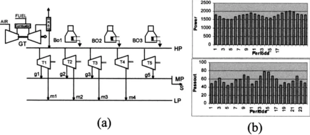
The utility system of Fig. 6(a) includes nine units

(steam turbines T1– T5, gas turbine GT and boilers

B1– B3) with efficiencies and capacities presented in

Table A2. The operating horizon consists of 24 equal-length periods. Each period relates to a pair of constant demands in power and process steam as shown in Table A3. Preventive maintenance imposes the shut-down of all units for one period. Optimal scheduling is expected to meet all demands and maintenance needs in the most economic way. Model properties are presented in Table 4.

The solution of the problem is addressed in two steps: I) preprocessing of the solution space and II) B&B customisation.

6.1. Step I

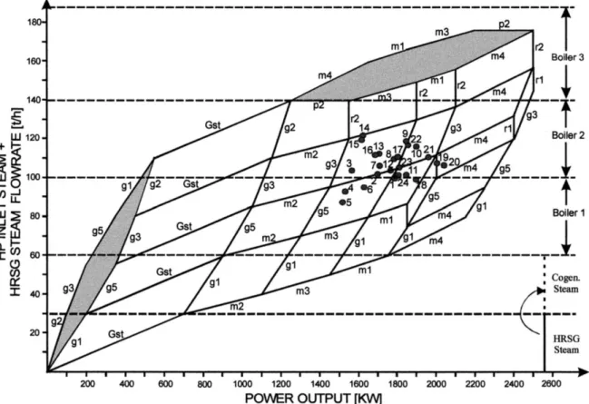
The solution space is analysed to reveal feasible and prioritised options. Preprocessing is applied in concep-tual and computational terms. The location of demands on the solution space (Fig. 7) in relevance to hardware limits identifies infeasible scenarios, which are excluded from optimisation. LP’s are solved to calculate penalties associated with the shut-down of units in feasible periods. Penalties in increasing sequence define priority lists OSuper. Penalties are also used for the unit

prioritisation list OSU. Ordered sets OSuper and OSU

formulate the Solver Matrix (Fig. 8) which encom-passes the prioritised solution space. The first column includes all units subject to maintenance arranged ac-cording to OSU(upper elements — GT, T2, T1, T3,… —

relate to higher priority units). Each element-unit of the first column associates to the corresponding period priority list OSuper defining the rows of the matrix.

Especially for OSTU4per the priorities between

zero-penalty periods are defined by insights of the

problem (period D has higher priority over the

rest since it is the least preferable for the mainte-nance of units TU1, TU2 and TU3).

(iii) Unit Prioritisation: The number of periods to consider for calculations ofPuaveruses the heuristic

rule of Eqs. (8) – (11): N(TU₁)=min

Penalties are applied for the first element of OSupen: TU1is assigned toPTU1aver=4433.3, followed

by TU3withPTU3aver=83.3. TU2and TU4have zero

first-period penalties. The priority list (first

itera-tion) is OSU={TU1, TU3, TU2– TU4}, where

TU2– TU4 represents units with identical Puaver.

An additional iteration considers the second ele-ments of OSTU2pen and OSTU4pen. TU3is now assigned

to value (888.9+0)/2 and TU4 to (0+0)/2. The

unit priority list is finally defined as:

OSU={TU1, TU3, TU2, TU4} (20)

From priority lists OSuper and OSU the Solver

Matrix is formulated: Æ Ã Ã Ã È TU₁ A C B TU₃ B A D C TU2 A C B D TU4 D C B A Ç Ã Ã Ã É

Step II: Application of the B&B solver:

The application of the customised solver selects can-didate problems and variables for branching, marks nodes for enumeration and deletes inferior nodes.

Un-Fig. 5. The development of the B&B tree for illustration.

Fig. 6. (a) Utility network and (b) sets of demands in power and heat for example problem.

6.2. Step II

The customised B&B searches the solution space according to the structure of the Solver Matrix. The branching of the binary tree initiates from the first elements of the upper rows and proceeds to deeper options only if specific properties hold. The enhanced pruning effectively disregards inferior parts of the tree from enumeration. The result is acceleration of the B&B algorithm compared with the solution of the same

Table 4

Model size for example problem

Binary Constraints

Continuous Non-zero

variables variables elements

754 2257

216 457

Fig. 7. Hardware composites depict the optimum solution space.

model by OSL implemented in GAMS (Brooke, Kendrick & Meeraus, 1992) as shown in Table 5.

OSL invested significant computational effort in searching the solution space. Even at the iteration limit of 150 000 optimality had not been reached due to the suboptimal flat profile the solver was trapped in. Alter-natively, the customised B&B performed better in all aspects and identified the optimal schedule after solving

(217+76) LP’s during Preprocessing and

Branching-and-Bounding, respectively. Optimal maintenance is performed according to vector:

(GT,T2,T1,T3,T5,B1,B2,B3,T4)

=(5, 15, 6, 4, 18, 4, 1, 19, 10) (22)

7. Conclusions

This work reports on the acceleration observed by customising the solution search to the special structure of problems. While the basic notions of the Branch-and-Bound, a widely applied algorithm for solving MILP’s, remain the same over the many contributions, computational experience has shown that general-pur-pose solvers can not capture special problem properties and are doomed to inferior performances. The design of inexpensive customised algorithms enhances

compu-tational efficiency and proves the superiority of such solvers over expensive commercial packages. It should be noted that the proposed methodology is generic

Fig. 8. The solver matrix encompasses the B&B customisation. Table 5

Computational results for example problem

Customised OSL(GAMS) B&B 188 50,402 Nodes 150 000 Iterations (Interrupted) 76 Solved LP’s 50 404 1339 3.2 CPU(s)-333 MHz

Objective-($/oper. horizon) 1 021 133.4 1 022 899.6 (Relaxed objective) (1 004 690) (1 005 439.7) Preprocessing Stage, 217 LP’s — 26.2 CPU(s).

within the context of the application, namely for ev-ery problem within the specification in the outline and problem description. The proposed approach car-ries intelligence to fully automate the customisation of the optimisation solver. Solution search engines with built-in intelligence and search technology perform better orders of magnitude. The ability to apply key B&B functions (branching, pruning) tailored to par-ticular solution spaces, speeds-up convergence and re-duces computational costs.

Appendix A

Boiler and Gas turbine models:

The cost of fuel burnt in a boiler (CFb), for

pro-ducing steam flowrate MSbis:

CF_b=B_fMS_b (A.1)

Slope (Bf) represents the incremental boiler efficiency.

The gas turbine is modelled by two interrelated lin-ear models that describe the relationship between the

steam (MSHRSG) in the Heat Recovery Steam

Genera-tor and the power output of the turbine (Eg):

MSHRSG=GstEg (A.2)

and a relation between the flowrate of the fuel burnt

in the combustion chamber and the steam (MS_HRSG)

raised in the HRSG:

CFg=GfMSHRSG (A.3)

Gst denotes the efficiency of raising HRSG steam and

Gf the turbine efficiency.

Problem Data:

Table A1: Operational parameters of turbines and boilers for illustration.

mtu[t/(hkW)] gtu[t/(hkW)] Bf[$h/(t(time Turbine horizon)] capacity:

power (kW)

mtu1=0.0125 gtu1=0.05 Bfb=2000 Turbine 3: 400

mtu2=0.0166 gtu2=0.0833 Turbine 4: 450

mtu4=0.03 gtu3=0.075

Table A2: Operational parameters of turbines and boilers for example problem.

mtu[t/(hkW)] gtu[t/(hkW)] Bf[$h/(t(time Boiler

horizon)] capacity [t/h] mtu1=0.0333 gtu1=0.15 Bfb1=523.3 Boiler 1: 40

Bfb2=534.16

mtu2=0.025 gtu2=0.3 Boiler 2: 40

Bfb3=555

gtu3=0.25 Boiler 3: 50

mtu3=0.02857

mtu5=0.05 gtu5=0.1667 Gf=562.5

Gst=0.042857 (t/hkW).

Table A3: Sets of demands in power and heat for example problem.

Demands

Power (kW) Process Steam [t/h]

Periods 49 1790 1 55 2 1700 62 1572 3 1535 4 52 45 1520 5 1682 6 50 58 7 1765 60 1790 8 70 9 1840 66 1910 10 1850 11 48 55 1780 12 1710 13 68 79 14 1630 77 1610 15 68 16 1690 61 1800 17 1900 18 46 52 2003 19 2030 20 49 56 21 1960 68 1860 22 56 23 1820 51 1800 24 Appendix B

Proof of Theorem 1:w1 is independent node [

B(w1)=B(w0)+p(u1,Tu₁ k(u1) )+p(u2,Tu₂ k(u2) )+… +p(un,Tu_n k(un)_{) (B.1)}

w%1 can be either independent node [

B(w%1)=B(w0)+p(u1,Tu₁ k%(u₁) )+p(u2,Tu₂ k%(u₂) )+… +p(un,Tu_n k%(u_n) ) (B.2)

or dependent node [ B(w%1)]B(w0)+p(u1,Tu₁ k%(u₁) )+p(u2,Tu₂ k%(u₂) )+… +p(un,Tu_n k%(un)_{) (B.3)}

All periods T present in w%1 are of lower or equal

priority than the corresponding ones of w1. Due to

priority sequence (k%(ui)]k(ui)), penalties: p(u1,Tu₁ k%(u1) )]p(u1,Tu₁ k(u1) ), p(u2,Tu₂ k%(u2) ) ]p(u2,Tu₂ k(u2) ), …,p(un,Tu_n k%(un)₎ ]p(un,Tu_n k(un)₎

The lowest possible value for B(w%1) (w%1 independent)

is always higher than B(w1):

B(w1)5B(w%1) (B.4)

The same proof applies for the case ofw2. The lower

bound B(w2) is given by Eq. (B.1), since the remaining

non-branched levels (X) do not contribute penalty

terms. It is similarly proven that:

B(w₂)5B(w%₂) (B.5) Proof of Theorem 2 Node w₁ is dependent (Tu_k k(uk) Tu_j k(uj)₎[_B(w 1) ]B(w₀)+p(u₁,Tu₁ k(u1)_)+p(u 2,Tu₂ k(u2)_)+… +p(uk,Tu_k k(u_k) )+…+p(uj,Tu_j k(u_j) )+… +p(un,Tu_n k(u_n) ) (B.6) [B(w1)=B(w0)+p(u1,Tu₁ k(u_j) )+p(u2,Tu₂ k(u₂) )+… +pag_((u k,uj),Tu_k k(u_k) )+…+p(un,Tu_n k(u_n) ) (B.7) wherepag_((u k,uj),Tu_k k(u_k)

is the aggregated penalty when more than one units are shut down in the same period.

Node w%1 is dependent (Tu_k k(u_k) Tu_j k(u_j) )[B(w%1) ]B(w0)+p(u1,Tu₁ k%(u1) )+p(u2,Tu₂ k%(u2) )+… +p(uk,Tu_k k(uk) )+…+p(uj,Tu_j k(uj)_)+… +p(un,Tu_n k%(un)_{) (B.8)} [B(w%1)=B(w0)+p(u1,Tu₁ k%(u1) )+p(u2,Tu₂ k%(u2) )+… +pag_((u k,uj),Tu_k k(uk) )+…+p(un,Tu_n k%(un)₎ (B.9)

All periods of node w%₁ are of lower or equal priority

than the corresponding ones of w₁ (k%(ui)]k(ui)) with

the exception of dependent periods Tu_k

k(u_k) Tu_j k(u_j) . As such, penalties p(u1,Tu₁ k%(u₁) )]p(u1,Tu₁ k(u₁) ),p(u2,Tu₂ k%(u₂) ) ]p(u2,Tu₂ k(u₂) ), …,p(un,Tu_n k%(u_n) )]p(un,Tu_n k(u_n) ), while (pag_((u k,uj),Tu_k k(u_k)

) is the same on both nodes. Compar-ing the two bounds becomes evident that:

B(w1)5B(w%1) (B.10)

Similarly for a pruned dependent node w2 where the

non-branched levels the B&B tree (X) do not contribute penalty terms it is proven that:

B(w2)5B(w%2) (B.11)

References

Brooke, A., Kendrick, D., & Meeraus, A. (1992). GAMS. A user guide,Release2.25. The Scientific Press.

Church, E. F. (1950). Steam Turbines (third ed.). New York: McGraw-Hill.

Dakin, R. J. (1965). A tree search algorithm for MILP problems. Computational Journal,8, 250.

Fabian, C.I. (1992). LINX: An interactive linear programming li-brary.

Floudas, C. A. (1995). Nonlinear and Mixed-Integer Optimisation, Fundamentals and Applications. Oxford University Press. Floudas, C.A. and Grossmann, I.E. (1995). Algorithmic approaches

to process synthesis: logic and global optimisation, American Institute of Chemical Engineering Symposium Series 304, Fourth International Conference on Foundations of Computer-Aided Process Design, Vol. 91, 198.

Friedler, F., Tarjan, K., Huang, Y. W., & Fan, L. T. (1992). Graph-theoretic approach to process synthesis: Axioms and the-orems.Chemical Engineering Science,47(8), 1973.

Friedler, F., Varga, J. B., & Fan, L. T. (1995). Decision-Mapping: a tool for consistent and complete decisions in process synthe-sis.Chemical Engineering Science,50(11), 1755.

Geoffrion, A. M., & Marsten, R. E. (1972). Integer programming algorithms: a framework and state-of-the-art survey. Manage -ment Science,18(9), 465.

Hooker, J. N., Yan, H., Grossmann, I. E., & Raman, R. (1994). Logic cuts for processing networks with fixed charges. Comput -ers Operations Research,21(3), 265.

Kearton, W.J. Pitman, (1958). Steam turbine theory and practice, 7th ed., London: Pitman.

Lee, S., & Grossmann, I. E. (2000). New algorithms for nonlinear generalised disjunctive programming. Computers and Chemical Engineering,24, 2125.

Mavromatis, S. P., & Kokossis, A. C. (1998a). A logic based model for the analysis and optimisation of steam turbine net-works.Computers in Industry,36(3), 165.

Mavromatis, S. P., & Kokossis, A. C. (1998b). Hardware Com-posites: A new conceptual tool for the analysis and optimisa-tion of steam turbine networks in chemical process industries. Part I: principles and construction procedure. Chemical Engi -neering Science,53(7), 1405.

Mavromatis, S. P., & Kokossis, A. C. (1998c). Hardware Com-posites: a new conceptual tool for the analysis and optimisation of steam turbine networks in chemical process industries. Part II: application to operation and design. Chemical Engineering Science,53(7), 1435.

Parker, G., & Rardin, R. (1988). Discrete Optimization. Academic Press.

Raman, R., & Grossmann, I. E. (1992). Integration of logic and heuristic knowledge in MINLP optimisation for process synthe-sis.Computers and Chemical Engineering,16(3), 155.

Raman, R., & Grossmann, I. E. (1993). Symbolic Integration of logic in Mixed-Integer Linear Programming Techniques for process synthesis.Computers and Chemical Engineering,17(9), 909. Raman, R., & Grossmann, I. E. (1994). Modelling and

computa-tional techniques for logic based integer programming.Computers and Chemical Engineering,18(7), 563.

Strouvalis, A. M., Mavromatis, S. P., & Kokossis, A. C. (1998). Conceptual optimisation of utility systems using hardware and comprehensive Hardware Composites. Computers and Chemical Engineering,22(Suppl.), 175.

Strouvalis, A. M., Heckl, I., Friedler, F., & Kokossis, A. C. (2000).

Customised solvers for the Operational Planning and Scheduling of Utility Systems.Computers and Chemical Engineering,24, 487. Turkay, M., & Grossmann, I. E. (1996). Logic-based MINLP al-gorithms for the optimal synthesis of process networks.Comput -ers and Chemical Engineering,20(8), 959.

Vecchiety, A., & Grossmann, I. E. (2000). Modeling issues and implementation of language for disjunctive programming. Com -puters and Chemical Engineering,24, 2143.

Vecchietti, A., & Grossmann, I. E. (1999). LOGMIP: a disjunctive 0-1 non-linear optimizer for process system models. Computers and Chemical Engineering,23, 555.